Robust point location estimators for the EWMA control chart

Abstract

In practice, the EWMA control chart for process monitoring is based on parameters estimated from a retrospective data set representing the process characteristic under study. This data set may contain contaminated observations, which in turn can affect the estimates and hence the control chart’s performance. We study the problem of estimating the location when the data set may or may not contain contaminated observations. We compare six point estimators proposed in the SPC literature. The quality of the estimators is evaluated in terms of estimation accuracy. Moreover, we study the impact of the estimators on the performance of the EWMA control chart based on the different location estimators.

Keywords:

• Contaminations
• EWMA control chart
• location estimators
• median
• Monte Carlo study
• Phase I
• Phase II
• robust
• statistical process control
• trimean

1. Introduction

Since its introduction by Roberts (1959), the exponentially weighted moving average (EWMA) control chart has become a well-known tool in statistical process control. The EWMA control chart and its properties have received much attention in the SPC literature. In practice, the in-control process parameters are unknown and have to be estimated. This stage is called Phase I. The monitoring stage is denoted by Phase II (cf. Vining, 2009).

The effect of Phase I estimation on the EWMA control chart was discussed by Jones (2002), Jones, Champ and Rigdon (2001), and Saleh, Mahmoud, Jones-Farmer, Zwetsloot, and Woodall (2015) who provided a design procedure for the EWMA control chart based on estimated Phase I parameters. These procedures use the sample mean and the sample standard deviation as estimators, yielding efficient parameter estimates. The application of such an EWMA control chart therefore requires the assumption that the Phase I data set contains only observations which are representative of the process.

However, it has long been recognized that in practical situations Phase I may occasionally contain contaminations, i.e. observations which are unrepresentative of the process such as outliers, step changes and other data anomalies (cf. Boyles, 1997 or Janacek and Meikle, 1997). In a literature survey of the effect of estimation on control chart properties, Jensen, Jones-Farmer, Champ and Woodall (2006) recommended studying robust or alternative Phase I estimators for μ and σ. This recommendation is the subject of our paper. We assess the effect of various estimators on the performance of the EWMA control chart when Phase I may contain contaminations.

To date, the literature has proposed several alternative estimators. For example, Rocke (1989, 1992), and Langenberg and Iglewicz (1986) studied robust point estimators for the Shewhart control chart. Schoonhoven, Nazir, Riaz and Does (2011) studied the effect of contaminations in Phase I and recommended the use of robust estimators for the Shewhart control chart. Nazir, Riaz, Does and Abbas (2013) compared robust point location estimators applied to another control chart, namely the cumulative sum control chart. For an overview, see Psarakis, Vyniou and Castagliola (2014).

In our paper, we compare the performance of the EWMA control chart based on various point location estimators in Phase I. In particular, we consider the situation in which Phase I may or may not contain contaminations. In the next section, we present the EWMA control chart and discuss the run length distribution as a performance measure. In Section 3, we describe the six location estimators, and in Section 4, we compare the accuracy of these estimators for a variety of contamination scenarios. In Section 5, we compare the effect of the location estimators on the EWMA control chart performance. Finally, Section 6 gives some concluding remarks.

2. Background information on the EWMA control chart

Our study involves the EWMA control chart for location. We assume that observations are collected in samples of size n and are identically independently and normally distributed with parameters μ and σ if the process is in control. Observations are denoted by Y_it, with i = 1, 2, … , n and t = 1, 2, 3, … .

The EWMA control chart consists of plotting the EWMA statistic Z_t together with the control limits. If the statistic lies within these limits, the process is said to be in control; otherwise a signal is observed and the process is assumed to be out of control. The EWMA statistic is defined as (1) where Y_t is the mean of sample t, , and λ, the smoothing parameter, is a constant satisfying 0 < λ ≤ 1. The upper and lower control limits for the EWMA control chart are (2) (3) where and are the Phase I estimates of μ and σ, and L is a positive coefficient which, together with λ, determines the in-control average run length of the EWMA control chart.

The run length (RL) is a random variable indicating the number of samples before Z_t falls outside the control limits. The performance of a control chart can be expressed in terms of the distribution function of the run length. For control charts with estimated parameters, a distinction is made between the conditional and unconditional run length distribution. The conditional run length gives the performance of the EWMA chart given the Phase I estimates. In order to evaluate the overall behavior, we consider the unconditional distribution of the run length. A common measure of control chart performance is the expected value of the RL, i.e. the average run length (ARL). It is desirable to have a large ARL when the process is in control and a small ARL when the process is out of control. Because the run length distribution is not geometric, as it is for Shewhart charts with known parameters, the ARL should not be used as the sole measure of chart performance. Therefore, we also evaluate the 10th, 50th and 90th percentiles of the unconditional run length distribution.

We take the following settings for the EWMA control charts: ARL = 370 when the process is in control and λ = 0.13. We set L = 2.89 as advised by Jones (2002). Before the EWMA control chart can be implemented, estimators for and need to be selected. In this paper, we consider EWMA control charts based on the six location estimators described in Section 2.

For a fair comparison of these location estimators, the standard deviation estimator for each chart is the same. We use an estimator of σ that is known for its robustness, namely a variant of the biweight A estimator proposed by Tatum (1997). This estimator weights the observations: higher values are given less weight than lower values, which ensures that outliers have less impact on the estimate of σ. The estimation procedure is described by Tatum (1997) and is implemented as set out in Schoonhoven, Riaz and Does (2011), with normalizing constant 1.068.

3. Phase I location estimators

Let X_it, with i = 1, … , n and t = 1, … , k, denote the Phase I observations. Define X_t as the mean of sample t, M_t as the median of sample t, X_(o)t as the oth-order statistic within sample t, and X_(o) as the oth-order value of the sample means. The Phase I data are used to obtain and , estimates of μ and σ, respectively.

The first location estimator that we consider is the mean of the sample means

This estimator provides a basis for comparison, as it is the most efficient estimator for in-control and normally distributed data. However, it is well known that this estimator is sensitive to data contaminations.

Second, we consider the trimmed mean of sample means. It was applied to control charting by Langenberg and Iglewicz (1986): trims α% of the ordered sample means from each tail and computes the mean of the remaining observations

Here ⌈ z ⌉ denotes the smallest integer not less than z. In this paper, we set α = 20%.

Next, we consider two estimators studied earlier by Rocke (1989). They are the median of the sample means and the mean of the sample medians

Furthermore, we include the median of the sample medians

Finally, we consider an estimator based on the sample trimean statistic (cf. Wang, Li & Cui, 2007) which is defined as a weighted average of the quartiles: TM_t = (X_(a)t + 2M_t + X_(b)t)/4, where a = ⌈n/4⌉ and b = n - a + 1. We consider a trimmed version of the mean of the sample trimeans where TM_(o) denotes the oth-order value of the sample trimeans. Again, we set α = 20%.

The estimators considered are listed in Table 1.

Table 1. Phase I location estimators.

Estimator	Notation
Mean of the sample means	̿X
Trimmed mean of the sample means	̿X20
Median of the sample means	MXt)
Mean of the sample medians	M
Median of the sample medians	M (Mt)
Trimmed mean of the sample trimeans	TMM20

4. Estimator efficiency in Phase I

We first discuss the accuracy of the proposed location estimators. Therefore, we conduct a simulation study in which we compare the mean squared error (MSE) of the estimators based on Phase I data consisting of k = 50 samples of size n = 5. The MSE is calculated as where μ^r is the value of the estimator in the rth simulation run and R is the total number of simulation runs.

We compare the six estimators as presented in Table 1 under four types of disturbances, where disturbances are reflected by changes in the process mean: out-of-control observations are drawn from N(μ + δ _I σ, σ ²), with δ_I a constant and the index ‘I’ indicating Phase I. If δ_I = 0, the process is in control; otherwise the process is out of control. Without loss of generality, we set μ = 0 and σ = 1, and consider

1. A model for localized shifts in which all observations in a sample have a 90% probability of being drawn from the N (0, 1) distribution and a 10% probability of being drawn from the N (δ_I, 1) distribution.

2. A model for diffuse shifts in which each observation, irrespective of the sample to which it belongs, has a 90% probability of being drawn from the N (0, 1) distribution and a 10% probability of being drawn from the N (δ_I, 1) distribution.

3. A model for structural shifts in which the first 45 samples are drawn from the N (0, 1) distribution and the last five samples are drawn from the N (δ_I, 1) distribution.

4. A model for random shifts in which, at random moments, five consecutive samples are drawn from the N (δ_I, 1) distribution. These shifts occur with a p × 100% probability. After this random shift of length 5, the process returns to the in-control state and every sample again has a p × 100% probability of being drawn from the N (δ_I,1) distribution. To have an expected contaminated rate of 10%, we set p = 0.023 (obtained through 100,000 simulations).

The performance of the proposed estimators is evaluated for δ^I = 0.25, 0.5, …, 3.5. The results are based on R = 100,000 simulations, which yields a maximum relative simulation error – the standard deviation of the R computed MSEs expressed as a percentage of the MSE – of 0.5%.

Figure 1 shows the MSEs plotted for each estimator against the shift size δ_I. The y-intercept represents the situation where all Phase I data are in control (δ_I = 0). The most efficient estimator is ̿X, as expected. All other estimators are slightly less efficient but still reasonably close to the MSE level of ̿X, except M(M_t), which is the least efficient estimator for uncontaminated data.

Figure 1. MSE of location estimators when contaminations are present in Phase I.

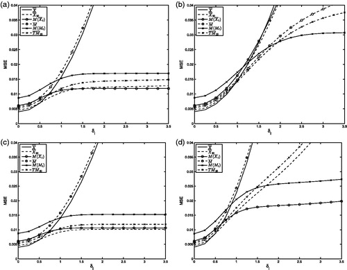
Next, consider the situations when contaminations are present. The MSE patterns of the six estimators are approximately equivalent for localized and structural shifts in Phase I. Hence, it does not matter for the estimators if the contaminated samples are spread randomly across Phase I (localized) or clustered at the end (structural). In both contamination scenarios, the estimators based on trimming (X₂₀ and TM₂₀) and the estimators which apply the median function to the samples (M(X_t) and M(M_t)) show low MSE levels, and are, therefore, the best-performing estimators.

In the random shifts scenario, the number of contaminated samples varies strongly and this causes a different MSE pattern. Here, only the estimators which apply the median function to the samples (M(X_t) and M(M_t)) show a low MSE level. The estimators based on trimming now show steeply increasing MSE levels. The reason is the additional variability in the number of contaminated samples in this scenario. Therefore, from the perspective of estimation accuracy, it is undesirable to use estimators based on trimming as these estimators lose their robustness as soon as the trimming percentage is occasionally lower than the contamination percentage.

When diffuse shifts are present, the MSE levels are high for all estimators compared with the other scenarios. The estimators which apply within-sample trimming, i.e. M, M(M_t) and TM₂₀, show the best performance for large shift sizes in Phase I.

To summarize, none of the location estimators have a satisfactory MSE performance for all the four contamination types. The estimators based on applying the median function or the trimean (M(X_t), M(M_t) and TM₂₀) show rather good performance for all four scenarios. However, M(X_t) breaks down for diffuse shifts as it does not trim within samples, M(M_t) is rather inefficient under in-control Phase I data, and TM₂₀ breaks down for random shifts as the number of contaminated samples occasionally exceeds 20%.

Finally, we also studied these estimators and Phase I performance for samples of size n = 10. The findings are comparable with the findings presented for n = 5, and are available upon request from the authors.

5. Comparison of Phase II EWMA control chart performance

Section 4 shows that the robust estimators offer substantial improvement over the efficient mean of sample means, if contaminations are present in Phase I. However, it remains to be shown that this translates into improved EWMA control chart performance. To do so, we compare the run length behavior of the EWMA control charts based on estimators using in-control as well as contaminated Phase I data. We conduct the following simulation study to obtain the RL behavior: first k = 50 samples of size n = 5 are drawn from the in-control N(0, 1) distribution and the four Phase I disturbance scenarios with δ_I = 1.5. Next, the mean and standard deviation are computed with the six location estimators for and Tatum’s robust estimator for . Based on these estimates, the EWMA control chart is set up according to Equations (1–3). Observations from N(δ_II, 1) are drawn until the associated Z_t falls outside the control limits. The corresponding run length equals t − 1. The calculations are made for δ_II = 0, 0.05, … , 0.6, where the index ‘II’ indicates Phase II. The entire procedure is repeated for R = 100,000 simulation runs. The obtained vector, of 100,000 RLs, gives the empirical unconditional run length distribution. The average run length and percentiles of this distribution for uncontaminated Phase I data and for the four contamination scenarios are reported in Table 2. Figure 2 shows the ARL plotted against a range of shift sizes δ_II for the EWMA control charts based on the six location estimators. Figure 2 also shows an extra dash-dotted line representing the ARL profile of the EWMA control chart based on ̿X given uncontaminated Phase I data. This profile serves as a benchmark for comparison, as it is the ARL profile if no contaminations occur in Phase I.

Figure 2. ARLs of the Phase II EWMA control chart when contaminations are present in Phase I.

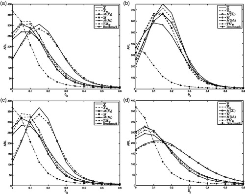
Table 2. ARL and percentiles of the RL distribution of the EWMA control chart with estimated parameters for k = 50, n = 5 and δ_I = 1.5.

Phase I		ARL and percentiles
		δII = 0				δII = 0.1				δII = 0.3				δII = 0.5
Contaminations		ARL	10th	50th	90th	ARL	10th	50th	90th	ARL	10th	50th	90th	ARL	10th	50th	90th
In-control	̿X(Benchmark)	369	26	199	899	208	14	90	511	21	3	14	44	6	1	5	13
	̿X20	357	25	188	870	208	13	89	521	21	3	14	45	7	1	5	13
	M(Xt)	331	22	168	819	210	12	86	531	24	3	14	48	7	1	5	13
	M	332	22	172	814	211	12	87	530	23	3	14	48	7	1	5	13
	M(Mt)	297	18	141	748	210	11	80	536	28	3	14	55	7	1	5	14
	TM20	342	23	176	839	212	13	87	528	22	3	14	47	7	1	5	13
Localized	̿X	139	8	48	340	280	16	127	707	136	8	47	330	17	2	10	34
	X20	260	15	113	650	318	20	157	790	54	5	23	112	10	2	7	20
	M(Xt)	264	15	115	671	288	17	136	726	52	5	21	108	10	2	7	19
	M	144	7	47	360	265	15	116	672	142	8	46	351	19	2	10	37
	M(Mt)	233	12	93	603	270	15	120	683	71	5	23	153	11	2	7	22
	TM20	243	14	103	623	307	19	149	765	61	5	24	128	10	2	7	21
Diffuse	̿X	208	13	75	486	630	34	280	1552	234	13	74	538	20	4	13	40
	X20	237	13	79	560	633	33	277	1572	227	12	69	521	20	4	13	40
	M(Xt)	263	13	79	652	599	29	248	1513	248	11	67	584	21	3	12	42
	M	321	15	100	796	651	33	286	1626	193	10	54	418	18	3	11	36
	M(Mt)	365	14	106	936	584	27	233	1478	205	8	48	463	20	3	11	38
	TM20	320	15	103	788	668	35	300	1680	181	10	53	393	17	3	11	35
Structural	̿X	112	9	49	260	318	21	159	786	111	9	48	258	14	3	10	30
	X20	267	17	123	667	334	22	172	818	45	5	23	97	9	2	7	19
	M(Xt)	273	16	124	685	299	18	144	746	47	5	21	97	9	2	7	19
	M	126	8	48	294	298	19	142	742	125	8	48	296	15	3	10	31
	M(Mt)	239	13	98	615	280	16	128	707	66	5	23	138	11	2	7	22
	TM20	253	15	112	640	325	21	164	802	52	5	24	110	10	2	7	20
Random	̿X	171	6	46	457	209	9	76	546	134	6	36	344	39	2	10	64
	X20	242	10	94	636	257	13	111	658	77	5	23	165	18	2	7	27
	M(Xt)	253	12	103	650	257	14	111	657	68	4	21	143	14	2	7	22
	M	166	5	45	443	204	8	72	536	134	6	35	346	40	2	10	67
	M(Mt)	220	9	81	580	237	12	95	607	84	4	23	192	18	2	7	28
	TM20	233	9	88	610	251	13	106	644	83	5	24	183	20	2	8	29

First, consider the situation where the Phase I data are uncontaminated (the upper part of Table 2). The EWMA control chart based on ̿X has an ARL of approximately 370, as it was designed to have, and a quickly declining out-of-control ARL. Furthermore, we see that the other EWMA control charts have a similar performance, i.e. they have comparable in-control and out-of-control ARLs. One exception is the control chart based on the robust estimator M (M_t), which falls short. This shows that using a very robust estimator purely based on the median is undesirable as it yields a control chart with a low ARL and low 50th percentile of the in-control run length, thus giving many more false alarms than expected if the data are actually in control.

Next, consider the situation where the Phase I data contain contaminations. A general observation is that, in the presence of contaminations in Phase I, the in-control ARL levels are much lower than the expected 370. Furthermore, all control charts are ARL-biased, i.e. the out-of-control ARL is larger than the in-control ARL (see Figure 2). The bias is large for diffuse shifts in Phase I and also if the EWMA control chart is based on the mean of sample means or mean of medians estimators (X and M). The estimators based on the median function or the trimean (M(X_t), M(M_t) and TM₂₀) yield the best – or least badly – performing EWMA control chart as they have rather high in-control ARLs and the smallest out-of-control ARLs if contaminations are present.

To summarize, contaminations in Phase I strongly determine the performance of the EWMA control chart. It will be biased and will have a smaller in-control ARL than the expected 370. However, the choice of the location estimator in Phase I does matter for the performance. We would advise not to use the traditional estimator X and recommend M(X_t). This yields an EWMA control chart with reasonable performance if localized, structural or random shifts are present in Phase I. Unfortunately, for diffuse shifts, none of the estimators yields an EWMA control chart with reasonable performance.

6. Concluding remarks

This article has studied several Phase I estimators of the location parameter which may be used for the EWMA control chart. We have focused on the impact of data disturbances in Phase I on the performance of the EWMA control chart in Phase II. Our study shows that data anomalies in Phase I can have a huge impact on the quality of the control chart. We have compared EWMA control charts based on six different location estimators, efficient as well as robust, and discovered that the use of the median of the sample means is a good alternative for the traditional mean of sample means estimator. The EWMA control chart based on the median of sample means shows reasonably good in-control performance and has the best performance if structural, random or localized shifts are present in Phase I. Note that, even though this estimator is the preferred estimator among the robust point estimators, the resulting Phase II EWMA control chart is still ARL-biased. More advanced estimation methods, such as screening data with control charts in Phase I or change point methods, can provide better estimates and hence unbiased Phase II EWMA control charts. See for example Zwetsloot, Schoonhoven, and Does (2014).

Disclosure statement

The authors report no conflicts of interest. The authors alone are responsible for the content and writing of this article.

Notes on contributors

Inez M. Zwetsloot, is a consultant of statistics at IBIS UvA and PhD student at the Department of Operations Management at the University of Amsterdam. She is working on her PhD on EWMA control charting techniques. Her e-mail address is [email protected].

Dr. Marit Schoonhoven, is a senior consultant of statistics at IBIS UvA. Her current research focuses on the design of control charts for non-standard situations. Her e-mail address is [email protected].

Dr. Ronald J. M. M. Does, is a Professor of Industrial Statistics at the University of Amsterdam, managing director of IBIS UvA and Director of the Institute of Executive Programmes at the University of Amsterdam. He is fellow of ASQ and ASA. His current research activities include the design of control charts for non-standard situations, health care engineering and Lean Six Sigma methods. His e-mail address is [email protected].

References

- Boyles, R.A. (1997). Estimating common-cause sigma in the presence of special causes. Journal of Quality Technology, 29, 381–395.
- Janacek, G.J., & Meikle, S.E. (1997). Control charts based on medians. Journal of the Royal Statistical Society: Series D (The Statistician), 46, 19–31.
- Jensen, W.A., Jones-Farmer, L.A., Champ, C.W., & Woodall, W.H. (2006). Effects of parameter estimation on control chart properties: A literature review. Journal of Quality Technology, 38, 349–364.
- Jones, L.A. (2002). The statistical design of EWMA control charts with estimated parameters. Journal of Quality Technology, 34, 277–288.
- Jones, L.A., Champ, C.W., & Rigdon, S.E. (2001). The performance of exponentially weighted moving average charts with estimated parameters. Technometrics, 43, 156–167.
- Langenberg, P., & Iglewicz, B. (1986). Trimmed mean X and R charts. Journal of Quality Technology, 18, 152–161.
- Nazir, H.Z., Riaz, M., Does, R.J.M.M., & Abbas, N. (2013). Robust CUSUM control charting. Quality Engineering, 25, 211–224.
- Psarakis, S., Vyniou, A.K., & Castagliola, P. (2014). Some recent developments on the effects of parameter estimation on control charts. Quality and Reliability Engineering International, 30, 1113–1129.
- Roberts, S.W. (1959). Control chart tests based on geometric moving averages. Technometrics, 1, 239–250.
- Rocke, D.M. (1989). Robust control charts. Technometrics, 31, 173–184.
- Rocke, D.M. (1992). XQ and RQ charts: Robust control charts. Journal of the Royal Statistical Society: Series D (The Statistician), 41, 97–104.
- Saleh, N. A., Mahmoud, M. A., Jones-Farmer, L. A., Zwetsloot, I. M., & Woodall, W. H. (2015). Another look at the EWMA control chart with estimated parameters. Journal of Quality Technology, 47, 363–382.
- Schoonhoven, M., Nazir, H.Z., Riaz, M., & Does, R.J.M.M. (2011). Robust location estimators for the X control chart. Journal of Quality Technology, 43, 363–379.
- Schoonhoven, M., Riaz, M., & Does, R.J.M.M. (2011). Design and analysis of control charts for standard deviation with estimated parameters. Journal of Quality Technology, 43, 307–333.
- Tatum, L.G. (1997). Robust estimation of the process standard deviation for control charts. Technometrics, 39, 127–141.
- Vining, G. (2009). Technical advice: Phase I and Phase II control charts. Quality Engineering, 21, 478–479.
- Wang, T., Li, Y., & Cui, H. (2007). On weighted randomly trimmed means. Journal of Systems Science and Complexity, 20, 47–65.
- Zwetsloot, I. M., Schoonhoven, M., & Does, R. J. M. M. (2014). A Robust Estimator of Location in Phase I Based on an EWMA Chart. Journal of Quality Technology, 46, 302–316.