Generalized offsetting of planar structures using skeletons

ABSTRACT

We study different means to extend offsetting based on skeletal structures beyond the well-known constant-radius and mitered offsets supported by Voronoi diagrams and straight skeletons, for which the orthogonal distance of offset elements to their respective input elements is constant and uniform over all input elements. Our main contribution is a new geometric structure, called variable-radius Voronoi diagram, which supports the computation of variable-radius offsets, i.e., offsets whose distance to the input is allowed to vary along the input. We discuss properties of this structure and sketch a prototype implementation that supports the computation of variable-radius offsets based on this new variant of Voronoi diagrams.

GRAPHICAL ABSTRACT

KEYWORDS:

• Weighted offset
• variable-radius offset
• generalized Voronoi diagram

1. Introduction

1.1. Constant and variable offsetting

Offsetting is an important task in diverse applications in the manufacturing business. For a set C in the Euclidean plane, the constant-radius offset with offset distance r is the set of all points of the plane whose minimum distance from C is exactly r. Formally, this offset can be defined as the boundary of the set , where denotes a disk of radius r centered at the point p. That is, the offset is the envelope of all disks of equal radius that have their centers along the input. Mathematically, the same offset can also be obtained as the Minkowski sum of C with a disk with radius r centered at the origin.

For polygons such a constant-radius offset will consist of one or more closed curves made up of line segments and circular arcs; see Fig. 1, left. Held [11] describes how to use a Voronoi diagram, which is a versatile tool in computational geometry, to compute such an offset efficiently and reliably for curvilinear inputs specified by straight-line segments and circular arcs. The underlying (generalized) Voronoi diagram is defined by the input line segments and circular arcs; it can be computed by the VRONI/ArcVRONI package [12].

Figure 1. (Left) The Voronoi-diagram (blue) of an input polygon P (black) enables efficient computation of the constant-radius offset. One interior offset curve of P is shown in green. The offset curve consists of line segments and circular arcs, and any point on it is at the same distance from the input in the standard Euclidean distance. (Center) The offset induced by the straight skeleton (blue) can have sharp corners that are far away from their respective input vertex in the standard Euclidean distance. (Right) Offsetting using the linear axis (blue) bevels the offset compared to the one induced by the straight skeleton. The offset still consists only of line segments.

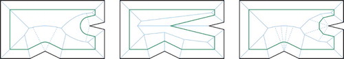
Mitered offsets differ from constant-radius offsets in the handling of non-convex vertices of an input polygon: Instead of adding circular arcs to the offset curve, the offset segments of the two edges incident to a non-convex vertex get extended until they intersect. This type of offset can be generated in linear time from a straight skeleton [16]. In order to avoid very sharp corners in the offset, the linear axis can be used in place of the straight skeleton [16], thus obtaining offsets with multi-segment bevels. See Fig. 1, center and right. State-of-the-art straight skeleton codes are presented by the authors [14,17].

A common feature of all these offsets is that the orthogonal distance of each offset element from its defining contour element is constant.

Several applications in industry, such as for garment manufacture or shoe design, need to construct differently sized pieces from a single master design. One obvious method is to scale the master template accordingly. However, a naive approach would scale all elements equally, which need not always be good enough. (For instance, one might want to shrink the overall size of a shirt without necessarily shrinking its collar size by the same ratio.) A different approach to resizing is to use offsetting. To be able to control the offsetting process, a common demand is to create non-constant offsets, i.e., offsets where the distance to the original input curve varies along that input. Brush stroke generation and the generation of ornamental seams are other sample applications that benefit of variable-distance offsets.

Variable-distance offset curves and surfaces are known in the literature. See, for instance, the work by Qun and Rokne [18] or Rossignac and Zhuo [19,21]. However, prior art seems to concentrate on defining and comparing different offsets and is less concerned with setting up a geometric framework that is general enough to support computing arbitrary offsets efficiently and robustly. One common approach applied in practice for constructing variable offsets seems to be based on sampling. Rendering-based methods also are feasible for sketching such offsets by means of graphics hardware; see, e.g., Li et al. [15]. However, rendering-based methods incur the additional problem of having to extract the actual offset curves from the rendered images.

1.2. Our contribution

We investigate skeletal structures that support the generation of offsets of planar straight-line graphs such that the orthogonal distance of an offset element from its defining input element is not necessarily uniform among all input elements, or even constant per input element. While weighted straight skeletons provide a natural means for computing offsets where the orthogonal distances are non-uniform but constant per input element, our investigations show that there is no obvious way to generalize them such that non-uniform and non-constant distances are supported.

Hence, we focus our attention on a generalization of Voronoi diagrams: We introduce variable-radius Voronoi diagrams of planar straight-line graphs and analyze properties of their bisectors. Similar to Voronoi diagrams in the case of constant-radius offsets, this structure captures all the information that is needed to compute variable-radius offsets efficiently. We conclude with discussing our proof-of-concept code for computing variable-radius Voronoi diagrams and sketch how offsetting can be extended to more general input primitives, such as circular arcs, in order to support variable-radius offsets that are piecewise continuous.

2. Generalized offsets based on straight skeletons

2.1. Straight skeletons and wavefront propagation

The straight skeleton of a simple polygon P is a skeletal structure first introduced to computational geometry by Aichholzer et al. [3] twenty years ago. It is similar to the Voronoi diagram but instead of being defined by a distance metric it is defined by a so-called wavefront propagation process.

Each edge of the polygon emits an edge of the wavefront towards the polygon's interior, moving at unit speed in a self-parallel manner. The polygons formed by these edges at any given time form the wavefront of P at time t.

Initially, at time t=0, the wavefront is identical to the input polygon. As the wavefront propagates and edges of the wavefront interact, the wavefront will have to be updated to maintain the simplicity of the wavefront. These changes are called events, and one can distinguish between two main types of events, namely edge events, which happen when an edge of the wavefront collapses to zero length and is removed from the wavefront, and split events which occur when a previously non-incident vertex “crashes” into the interior of a wavefront edge and, thus, the wavefront polygon is split into two portions.

This propagation process continues until all elements of the wavefront have collapsed. The straight skeleton then is defined as the geometric graph whose edges are the traces of wavefront vertices over the propagation period; see Fig. 2. It is customary to refer to edges of the straight skeleton as arcs and to call its vertices nodes to distinguish them from input or wavefront edges and vertices. The straight skeleton tessellates the input polygon into non-overlapping faces. We refer to Huber [13] for a detailed discussion of straight skeletons; recent algorithms and codes by the authors for computing straight skeletons are documented in [14, 17].

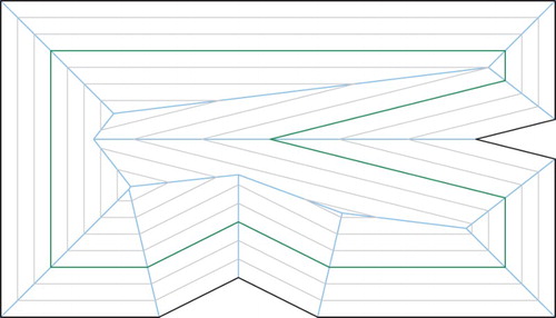
Figure 2. A simple polygon (black) and a family of wavefronts, i.e., mitered offset curves, at equidistant time intervals (gray). The straight skeleton (blue) traces the vertices of the wavefront over time. One offset is shown in a more distinct dark green.

The weighted straight skeleton is a generalization of the straight skeleton first mentioned by Aichholzer and Aurenhammer [2] and Eppstein and Erickson [10]. Wavefront edges no longer necessarily move at unit speed, but instead move at different speeds corresponding to individual edge weights; see Fig. 3. Several properties of weighted straight skeletons, such as whether faces remain monotone to their input site, were only very recently investigated by Biedl et al. [7, 8].

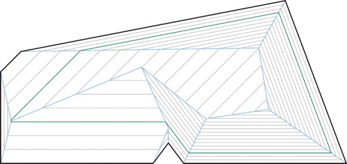
Figure 3. The weighted straight skeleton (blue) of a polygon (black) with a family of offset curves (gray, green).

2.2. Offsetting using straight skeletons

Straight skeletons provide a natural and efficient instrument to obtain mitered offset curves. Palfrader and Held [16] demonstrate that Aichholzer and Aurenhammer's triangulation-based algorithm [2] for computing unweighted straight skeletons can be implemented robustly on standard IEEE 754 double-precision floating-point arithmetic. Their experiments show that computing the straight skeleton of inputs of a million vertices takes under ten seconds, and that mitered offsets can be computed in fractions of a second if a straight skeleton is available.

Their approach for obtaining unweighted mitered offsets from the unweighted straight skeleton generalizes naturally to offsetting with variable distances using the weighted straight skeleton. Both unweighted and weighted offsets consist of straight-line segments only. Each of these line segments is parallel to its corresponding input segment, at a distance proportional to the input segment's weight.

While the offsetting distance can be varied by input segment, it does not change along a single input segment. We point out that it is not possible to achieve such a variation by splitting an input segment into multiple smaller collinear segments with variable weights: As soon as collinear wavefront segments become incident, the wavefront propagation requires that a single preferred - say the fastest or the slowest - wavefront segment takes over the corresponding portion of the wavefront [7]. Even slight perturbations would not produce the desired result as the fastest wavefront edge would almost immediately dominate the wavefront.

2.3. Generalized skeletons based on non-parallel wavefront edges

In the standard weighted straight skeleton described above, input segments are assigned a weight and then wavefront edges propagate at speeds that correspond to these weights. These weights imply specific velocities for the wavefront vertices: Each wavefront vertex moves along a bisector with the velocity, i.e. speed and direction, necessary to “keep up” with the propagating wavefront edges.

To introduce non-parallel offset segments one might be tempted to assign velocities directly to the wavefront vertices. Unfortunately, offsets defined based on such an approach suffer from two problems that diminish their practical applicability.

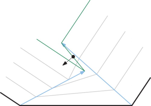
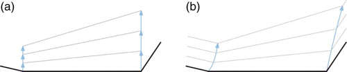
First of all, such a setup may cause offset segments to rotate during the wavefront propagation such that the inwards normal of an offset segment is actually pointing towards the input segment instead of away from it: See the dotted normal in Fig. 4. Furthermore, an offset for some time t may intersect an offset of some later time : the green offset in Fig. 4 intersects the previous one.

Figure 4. Picking velocities of wavefront vertices will result in undesirable behavior such as offset segments rotating or offsets from different times intersecting each other.

To avoid the problems that arise when assigning velocities directly to the wavefront vertices, one could try to instead specify an orthogonal propagation speed at the endpoints of each input segment; see Fig. 5. This seems promising when just looking at the offset segments. However, such a setup results in wavefront vertices that no longer move along straight lines. Thus, the arcs of the underlying skeletal structure will not be straight-line segments either. Therefore it seems unlikely that the theory of straight skeletons will be of much help in understanding or even constructing such structures. To overcome this problem we resort to generalized Voronoi diagrams; they will provide adequate support for the generation of generalized offsets with non-constant distances.

Figure 5. (Left) Propagation speed of the wavefront emanated from the lower middle input segment. (Right) Three offsets as a result of such a propagation scheme. Picking a variable orthogonal propagation speed will result in reasonable offsets again. However, the arcs of this skeletal structure are no straight-line segments and the theory of straight skeletons is no longer applicable.

3. Generalized offsets based on Voronoi diagrams

3.1. Preliminaries

The Voronoi diagram of a set S of points in the plane, called sites, tessellates the plane into interior-disjoint regions. Each so-called Voronoi region belongs to exactly one site. The Voronoi region of a site s is given by the loci of all points in the plane whose closest site is s. The prairie-fire analogy illustrates this concept nicely: Suppose that fires start at different point locations on the prairie and that each fire expands into all directions, propagating at uniform speed. A point in the prairie then belongs to the Voronoi region of the particular fire which reached it first. The border between any two Voronoi regions lies on a straight line, namely the bisector of the regions' sites; see Fig. 6, left.

Figure 6. (Left) The Voronoi diagram of a point set. Each site's Voronoi region is shaded in a different color. (Right) A multiplicatively weighted Voronoi diagram of the same point set. Vertices marked with □ have been assigned a weight of 3.0, those marked with × have weight 1.5, while the vertices shown with • have a weight of 1.0. The bisectors of vertices of different weights lie on circular arcs. Note that some Voronoi regions are disconnected.

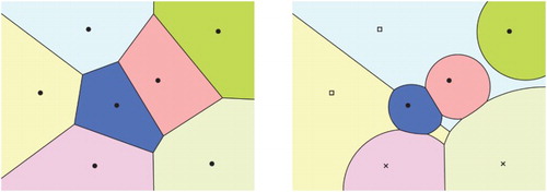
Voronoi diagrams have been generalized in several different ways, such as using a different distance measure (e.g., Manhattan distance instead of Euclidean distance), choosing different types of input sites instead of just points (e.g., line segments or circular arcs), or assigning both additive and multiplicative weights to sites. In the prairie-fire analogy, the latter generalization corresponds to starting certain fires sooner or have some spread faster. Figure 6, right, shows the Voronoi diagram of a multiplicatively weighted point set. We refer to Aurenhammer and Edelsbrunner [6] for an algorithm for computing weighted Voronoi diagrams.

3.2. Variable-radius offset

Now consider a set S of vertices in the Euclidean plane and line segments between some pairs of these vertices. The line segments may share common endpoints but they may not intersect otherwise. (In computational geometry, such an input is called a planar straight-line graph, PSLG.) Let us denote by the set of points covered by all vertices and line segments of S. Furthermore, we consider a weight function defined in the following way:

• To each vertex p of S some non-negative weight is assigned.

• Then, for a point f on a line segment of S, with for some , the weight is given by .

That is, after assigning weights to all vertices of S, the weights for points on segments of S are obtained by a linear interpolation of the corresponding vertex weights.

To motivate the definition of the offsets we recall the prairie-fire model. However, now we allow fires to propagate at different speeds. Then the boundary of the area burnt by the fire would give the offset. Hence, at each point p of we place a wavefront disk whose radius grows over time. Initially all disks have radius zero. As time increases the radius of each disk grows proportional to the weight of its center point . The variable-radius offset for a given time is the envelope of this set of disks. As intended, input sites with small weight will induce an offset that is closer to them, and input sites that were assigned larger weights will cause their offsets to be farther away.

Similar to the standard constant-radius offset, the variable-radius offset can be seen as a generalized Minkowski sum: It is the boundary of the set . Note that the term replaces the constant radius r in the standard Minkowski sum. Since, by its very definition, the offset distance along a variable-radius offset curve varies, we find it more convenient to refer to the time t than to a distance to characterize variable-radius offsets.

3.3. Variable-radius Voronoi diagram

We now turn our attention to a skeletal structure which, similar to Voronoi diagrams and straight skeletons in the case of constant-radius and mitered offsets, captures the geometry of variable-radius offsets. The set S of input sites is a set of both vertices and (non-intersecting) line segments between pairs of these vertices, i.e., a planar straight-line graph. We introduce the variable-radius Voronoi diagram of S as a generalized Voronoi diagram with one main generalization:

• We assign multiplicative weights to these sites. As described above, a vertex is assigned a weight , and the weight of a point on a line segment changes linearly between its vertices from to .

All weights are assumed to be non-negative. (In a practical application all weights will be strictly positive.)

The distance of a point u in the plane to a vertex site is defined as the Euclidean distance from u to s, divided by the weight of that site: where denotes the standard Euclidean length of the straight-line segment between u and s. The distance of u to a line-segment site is naturally defined as the minimum distance of u to any point of the line segment: While this may seem unwieldy at first, we show below that can be computed easily using elementary geometry.

As in the case of the standard Voronoi diagram, every point in the plane is in the (generalized) Voronoi region of the site that it is closest to. An arc that separates two regions comprises all points that have the same distance to two sites and a larger distance to all other sites.

The variable-radius Voronoi diagram inherits several important properties from the multiplicatively weighted Voronoi diagram of points. In particular, the region of a given site need not be connected, cf. Fig. 6 (right). That is, the region of a site may comprise two or more disconnected faces in the Voronoi diagram. Furthermore, bisectors between two vertices are circles or circular arcs [6]. Other bisectors, however, are more complex curves in general. A special case is given by the bisector between a vertex and a line segment of constant weight: It will be a conic section where the vertex site is the focus point and the supporting line of the segment site is the directrix of the conic. Depending on the ratio of the weights of the segment and the vertex, the bisector will either be an ellipse, a parabola, or a hyperbola.

To better understand the shape of variable-radius offset curves and bisectors, we start with investigating the wavefront propagation defined by one weighted line segment and its two weighted vertices. We will establish that the offset of a line segment is again a line segment. To simplify matters even further, we begin with studying weighted line segments where one vertex has a weight of zero, and then we will continue with showing that the general case is very similar.

3.3.1 A line segment with zero weight on one end

Consider the line segment , with and . What is the region of the plane that is reached from a wavefront sent out from this line segment after a certain time t has elapsed? What is the boundary of this region, i.e., the offset curve that corresponds to this particular time?

Since , for sufficiently large values of t the area bounded by the offset curve will be a disk centered at q: The larger growth rate of the wavefront disk centered at q implies that it dominates all growing disks centered along other points of . The answer is less obvious for sufficiently small values of t when this area is not yet a disk.

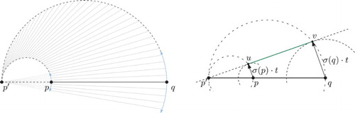
So, consider a time t for which the area covered by the wavefront is not yet a disk. We call those values of t permissible time values; we will shortly see how to determine the interval of permissible time values. Let . Hence, λ equals the radius of the wavefront disk at time t centered at the vertex q. Furthermore, let L be a line through p that is tangent to . We denote the touching point of L and by v; see Fig. 7.

Figure 7. An offset (green) of a weighted line segment where the weight of p is zero. The circular arc T separates the Voronoi region of the (open) line segment from the Voronoi region of the vertex q.

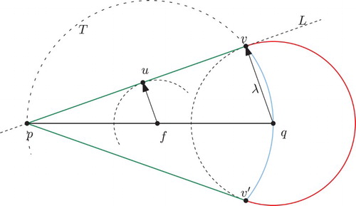
Let u be an arbitrary point on , and let . Thus, u partitions into and such that . Let f be the point on given as . By the Intercept Theorem, and, therefore, is tangent to L. Since the weight along line segments is interpolated linearly, we observe that the weight of point f is . Thus, .

Now recall that our choice of u on was arbitrary. It follows that for any point u on we can find a unique point f on such that touches L tangentially in u. Conversely, for any f on there is exactly one point u on that is covered by the disk .

Any point beyond v on the supporting line of is too far away to have been reached at time t from any wavefront disk centered at some point of . We conclude that the area covered by proportionately sized disks along comprises the triangles and as well as the disk . Of course, the boundary of this area consists of the two line segments and and of one circular arc. See the green and red entities in Fig. 7.

3.3.2 Partitioning into Voronoi regions

We prefer to regard the input site as the open line segment between p and q, exclusive of p and q, since this allows a meaningful partitioning of the area covered by the wavefront at time t. Then the circular arc section of the offset belongs to the input site q alone, and the two straight-line segments are the offset segments of . Hence, the offset of a weighted straight-line segment is indeed again a line segment and the offset of a vertex is a circular arc.

Note that the offset of the weighted line segment vanishes as soon as the wavefront disk of q dominates all other wavefront disks. Of course, this happens when the wavefront disk of q reaches p. Since the radius of this disk is given by for time t, we get as the time when the offset of turns into a disk. The permissible time interval in the case of is therefore .

Furthermore, if we consider , the area traced out by offsets of the open segment is the open disk whose diameter is . We call this disk the area of influence of . In this simple example, the area traced out by offsets of q is the remaining rest of the plane.

3.3.3 Finding the weighted distance of a point to a line segment

Again, consider an input line segment where . Given a point u in the area of influence of , how can we determine the weighted distance and, thus, also the time t such that u lies on the offset of at time t?

Construct the line L through p and u, then construct the circle T whose diameter is . The intersection of L and T is denoted by v. By Thales' Theorem, and are orthogonal; see Fig. 7. We find that the wavefront emanated by has reached u at time .

3.3.4 Line segments with constant weights

Once more, we consider a line segment but now we no longer restrict to zero. We can distinguish between two cases depending on whether or not. If the line segment is of uniform weight, then the offsets of at time t are copies of the original line segment, moved orthogonally by ; see Fig. 8.

Figure 8. The offsets of a uniformly weighted line segment (gray).

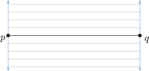
Figure 9. (Left) The offsets (gray) of a weighted line segment . The supporting lines of all offset segments meet in a common point on the supporting line of . The bisectors exhibit another interesting property: They are full circles whose diameters on the line supporting are bounded by and their individual defining point site. (Right) Using the Intercept Theorem we can compute the position of on the supporting line of .

3.3.5 Line segments with variable weights

If, however, the weights of the two vertices p,q differ, i.e., if , then this case can be treated similar to the case where one weight was zero.

Assume, without loss of generality, that . We consider the two wavefront disks and for all those values of t for which the disk centered at p is not entirely contained in the disk centered at q. Again, we call these the permissible time values of t.

The Intercept Theorem implies that all lines which are tangent to both and will intersect the supporting line of in a common point ; see Fig. 9. Note that this holds for all permissible values of t. To compute the position of , we note that the triangles and are similar. Thus, . We substitute with , solve for , and find that the point is the distance away from p.

The offset of at time t is therefore on the same supporting line as the offset of at time t, with , but it is bounded on the side of p by the arc sent out by p. We conclude that the Voronoi region of p is a disk whose diameter is , the Voronoi region of the open segment is a disk whose diameter is without the region of p, and the Voronoi region of q is the entire rest of the plane. See also Fig. 10, left.

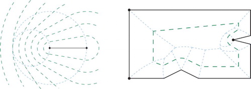
Figure 10. (Left) The variable-radius Voronoi diagram (blue, dotted) of a simple input of two vertex sites and their connecting line segment (black). A family of offset curves is shown in green (dashed). (Right) The variable-radius Voronoi diagram inside a polygonal input. The marked input vertices on the left have been assigned a weight of 2.0 while the single marked vertex on the right has a weight of 0.5. All other vertices were given the standard weight of 1.0. A single offset curve is drawn in green.

The point is also the point that is reached at the same time by the wavefronts emanated from p and q and from every point on . Therefore, the permissible time interval is , or equivalently, .

3.3.6 Bisectors of a variable-radius Voronoi diagram

The bisector between a pair of weighted points is a circle, which is a property inherited from multiplicatively weighted Voronoi diagrams of point sets. This is easy to see if we recall that ancient Apollonius of Perga showed that a circle is the set of points of a fixed ratio of distances to two foci. The two foci in this case are the two input sites, and their bisector is the Apollonian circle which traces out the ratio of their two weights. This argument also provides a second explanation as to why the bisector between an (open) line segment and either of its incident vertices is a circle: This bisector is the limiting case of the Apollonian circle of the vertex and an infinitesimally close point on the line segment with proportionally infinitesimally smaller or larger weight.

Unfortunately, the bisectors between vertices and non-incident segments or between two line segments are not nearly as nicely behaved. Rather, they are higher-order curves that are cumbersome to parameterize.

3.4. Offsetting

While the bisectors of consist also of non-trivial curves, the variable-radius offset itself comprises line segments and circular arcs only. In particular, in Voronoi regions that belong to line-segment sites the offset will also be a line segment (see the previous section), whereas in regions associated with vertices the offset element will be a circular arc; see Fig. 10, right.

We can compute this variable-radius offset of S for a given time t from the variable-radius Voronoi diagram . The approach is identical to how constant-distance offsets are computed based on Voronoi diagrams or straight skeletons [11,16]. Roughly, we iterate through all the arcs of and add offset elements in each face that contains points at distance . The topological information encoded in enables us to do this in time linear in the size of the Voronoi diagram and in a single iteration, without the need to compute all pair-wise self-intersections of offsets. Furthermore, no detection and removal of invalid loops is required even for large offset distances.

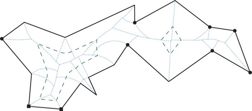
For instance, in Fig. 11 the offset distance chosen is large when compared to the feature size of parts of the polygon. A simple inspection of the numerical data associated with the Voronoi diagram shows that some Voronoi arcs and faces on the right-hand side of the polygon do not contain points at the offset distances sought. That is, the availability of the variable-radius Voronoi diagram suffices to infer that no offset segments and arcs need to be added there.

Figure 11. Another variable-radius Voronoi diagram of a polygonal input with vertex weights of 2.0 (disks), 0.5 (squares), and 1.0 (unmarked vertices). One offset is drawn in green. Note that it consists of two components.

3.5. Implementation

Edelsbrunner and Seidel [9] established the connection between Voronoi diagrams in with lower envelopes in . Setter et al. [20] used this connection to add a powerful tool to CGAL [1] for computing Voronoi diagrams via lower or upper envelopes of suitably formed surfaces in 3D. For the point set Voronoi diagram it is well known that these surfaces are cones, and extending this to weighted point sets is readily done by varying the dihedral angle of these cones.

The variable-radius Voronoi diagram inherits cones as the surfaces of vertices from the weighted point set Voronoi diagram. The surfaces that correspond to line segments are more involved. We have shown that the offset of a line segment is again a line segment. If we consider a family of offset segments of an input segment and lift each offset segment along the z-axis by a distance that corresponds to the time when it was reached by the wavefront, we obtain a ruled surface. Recall that the supporting lines of all offsets intersect at a common point on the supporting line of the input site. Therefore, our ruled surface actually is a sub-surface of a right conoid. That is, it is a ruled surface generated by straight lines that all intersect a fixed straight line, the axis, perpendicularly.

CGAL's 3D envelope computation algorithm is generic in the sense that it can deal with arbitrary terrain surfaces as long as it has some means to learn about certain geometric properties of those surfaces. The algorithmic back-end calls a user-supplied traits-class which is responsible for answering queries such as which of two 3D surfaces has a larger z-coordinate above a given point p on the xy-plane.

Our current implementation is based on CGAL and supports an approximate computation of the variable-radius Voronoi diagram. However, CGAL also provides the machinery required for an implementation of an exact version, albeit with some additional engineering work.

Since our proof-of-concept implementation has not yet been engineered for speed or robustness, we refrain from presenting any performance statistics here.

3.6. Extending beyond polygonal input

So far we have limited ourselves to input sites that are either points or line segments. Generalizing the class of input sites would be useful for supporting offsets that are (piecewise) continuous for appropriate inputs.

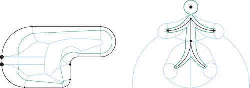
Currently, we can handle circular arcs by sampling them; see Fig. 12. Note that the offset of a variable-weighted circular arc is not a circular arc. Therefore, for supporting circular arcs directly, a better understanding of the mathematical characteristics of the corresponding Voronoi bisectors and of the resulting offsets would be required.

Figure 12. Variable Voronoi diagrams with one offset curve. The size of vertex markers is proportional to their weight.

4. Conclusion

We investigate a new geometric structure which we call variable-radius Voronoi diagram. While this structure is of sufficient theoretical interest on its own grounds, we demonstrate its practical applicability to constructing variable-radius offsets, i.e., a specific variant of offsets for which the orthogonal distance to the input is allowed to vary along the input. Our prototype implementation supports the computation of variable-radius offsets for general planar straight-line graphs. With some extra amount of work it could be generalized to support curvilinear input defined by straight-line segments and circular arcs.

From a theoretical point of view, it would be possible to extend the class of input sites allowed even beyond circular arcs to more general primitives such as conics or splines. However, for such a generalization care has to be taken to handle sites correctly once they themselves have a non-empty medial axis. One feasible approach to overcoming this problem would be to deal with only those primitives which also form so-called ”harmless curves”, as defined by Alt and Schwarzkopf [5]. The more recent paper by Alt, Cheong and Vigneron [4] presents a randomized-incremental algorithm for computing the Voronoi diagram of n such curves in time.

Acknowledgments

This work was supported by Austrian Science Fund (FWF): P25816-N15.

ORCID

Martin Held http://orcid.org/0000-0003-0728-7545

Stefan Huber http://orcid.org/0000-0002-8871-5814

Peter Palfrader http://orcid.org/0000-0002-5796-6362

References

- CGAL; Computational Geometry Algorithms Library. http://www.cgal.org/
- Aurenhammer, O.; Aichholzer, F.: Straight Skeletons for General Polygonal Figures in the Plane. A. Samoilenko (Editor), Voronoi's Impact on Modern Sciences II, volume 21. Institute of Mathematics of the National Academy of Sciences of Ukraine, Kiev, Ukraine, 1998, 7–21. doi: 10.1007/3-540-61332-3_144
- Aichholzer, O.; Aurenhammer, F.; Alberts, D.; Gärtner, B.: A Novel Type of Skeleton for Polygons, J. Univ. Comp. Sci19951(12752–761. doi: 10.1007/978-3-642-80350-565.
- Alt, H.; Cheong, O.; Vigneron, A.: The Voronoi Diagram of Curved Objects, Discrete Comput. Geom., 34(3), 2005, 439–453. doi: 10.1007/s00454-005-1192-0.
- Alt, H.; Schwarzkopf, O.: The Voronoi Diagram of Curved Objects. Proc. 11th Annu. ACM Sympos. Comput. Geom. 1995, 89–97. doi: 10.1145/220279.220289>
- Aurenhammer, F.; Edelsbrunner, H.: An Optimal Algorithm for Constructing the Weighted Voronoi Diagram in the Plane, Pattern Recognition, 17(2), 1984, 251–257. doi: 10.1016/0031-3203(84)90064-5
- Biedl, T.; Held, M.; Huber, S.; Kaaser, D.; Palfrader, P.: Weighted Straight Skeletons in the Plane, Comp. Geom.: Theory and Appl., 48(2), February 2015, 120–133. doi: 10.1016/j.comgeo.2014.08.006
- Biedl, T.; Huber, S.; Palfrader, P.: Planar Matchings for Weighted Straight Skeletons. H.-K. Ahn; C.-S. Shin (Editors), Proc. 25th Int. Sympos. Alg. & Comp. (ISAAC 2014), LNCS, volume 8889. Springer, Jeonju, Korea, December 2014, 117–127. doi:10.1007/978-3-319-13075-0_10
- Edelsbrunner, H.; Seidel, R.: Voronoi Diagrams and Arrangements, Discrete Comput. Geom., 1(1), December 1986, 25–44. doi: 10.1007/BF02187681
- Eppstein, D.; Erickson, J.: Raising Roofs, Crashing Cycles, and Playing Pool: Applications of a Data Structure for Finding Pairwise Interactions, Discrete Comput. Geom., 22(4), 1999, 569–592. doi: 10.1145/276884.276891
- Held, M.: On the Computational Geometry of Pocket Machining, LNCS, volume 500. Springer, 1991. doi:10.1007/3-540-54103-9. ISBN 978-3-540-54103-5
- Held, M.: VRONI and ArcVRONI: Software for and Applications of Voronoi Diagrams in Science and Engineering. Proc. 8th Int. Sympos. Voronoi Diagrams in Sci. & Eng. (ISVD 2011). Qingdao, China, June 2011, 3–12. doi: 10.1109/ISVD.2011.9>
- Huber, S.: Computing Straight Skeletons and Motorcycle Graphs: Theory and Practice. Shaker Verlag, 2012. ISBN 978-3-8440-0938-5
- Huber, S.; Held, M.: A Fast Straight-Skeleton Algorithm Based On Generalized Motorcycle Graphs, Int. J. Comp. Geom. Appl., 22(5), October 2012, 471–498. doi: 10.1142/S0218195912500124
- Li, C.; Zhou, G.; Chan, C.: A Graphical Approach to Approximate Offset Computation. Proc. Sixth Conf. Comput. Graph., Imag. Visualization. August 2009, 217–221. doi: 10.1109/CGIV.2009.46>
- Palfrader, P.; Held, M.: Computing Mitered Offset Curves Based on Straight Skeletons. Comp.-Aided Design & Appl., 2015. doi: 10.1080/16864360.2014.997637>. In print
- Palfrader, P.; Held, M.; Huber, S.: On Computing Straight Skeletons by Means of Kinetic Triangulations. L. Epstein; P. Ferragina (Editors), Proc. 20th Annu. Europ. Symp. Alg. (ESA 2012), LNCS, volume 7501. Springer, Ljubljana, Slovenia, September 2012, 766–777. doi: 10.1007/978-3-642-33090-2_66>
- Qun, L.; Rokne, J. G.: Variable-Radius Offset Curves and Surfaces, Mathl. Comput. Modelling, 26(7), October 1997, 97–108. doi: 10.1016/S0895-7177(97)00188-X
- Rossignac, J.: Ball-Based Shape Processing. I. Debled-Rennesson; E. Domenjoud; B. Kerautret; P. Even (Editors), Proc. 16th Int. Conf. Discrete Geom. Comp. Imagery (DCGI 2011), LNCS, volume 6607. Springer, Nancy, France, April 2011, 13–34. doi:10.1007/978-3-642-19867-0_2
- Setter, O.; Sharir, M.; Halperin, D.: Constructing Two-Dimensional Voronoi Diagrams via Divide-and-Conquer of Envelopes in Space. M. L. Gavrilova; C. J. K. Tan; F. Anton (Editors), Transactions on Computational Science IX, LNCS, volume 6290. Springer, 2010, 1–27. doi: 10.1007/978-3-642-16007-3_1>
- Zhuo, W.; Rossignac, J.: Curvature-based Offset Distance: Implementation and Applications, Computers & Graphics, 36(5), August 2012, 445–454. doi: 10.1016/j.cag.2012.03.013