Sensitivity coefficients for experimental estimation of interstitial properties during phase change in porous media

Abstract

The sensitivity coefficients for analyzing the interstitial properties during phase change in porous media are presented. Computation of the sensitivity coefficients and estimation of parameters are the main objective of this study. Experimentally measured temperature data provide an estimate of the phase front locations used as the state variable for this study. The derivations are based on the assumption that the phase front, X, at a given time, t, is a function of interstitial properties τt and τq with all other parameters remaining constant. The properties τt and τq are the lag-time in temperature and heat flux, respectively. The study of the sensitivity coefficients using these two parameters is the objective of this study. The analysis includes two types of boundary conditions of the first kind: prescribed temperature of phase change materials and prescribed temperature for solid matrix. These boundary conditions are related to the conditions under which the experimental data used in this article were collected. The results confirm the existence of the local thermal non-equilibrium condition at the onset of a phase change phenomenon.

Keywords:

• Sensitivity coefficients
• Interstitial properties
• Phase change
• Porous media
• Parameter estimation

1. Introduction

Mathematical models are often formulated to describe and elucidate the behavior of an engineering system, and also to illustrate quantitatively available experimental data. These models are often represented in the form of a complex, multi-parameter partial differential equation. In most cases, the correlation between the parameters and the state variables are not known a priori. This information is needed to gain understanding of the response of the state variable to alteration in the parameters. The partial derivative of the state variable with respect to the parameters is referred to as the sensitivity coefficient. Sensitivity coefficients are very useful in parameter estimation [1,2], optimal experimental design [3,4], and uncertainty or error analysis [5,6]. The determination of the sensitivity coefficient for analyzing interstitial properties during phase change in porous media is the subject of this investigation.

Phase change phenomena in porous media are often encountered in numerous science and engineering applications. These include melting and freezing of biological tissue, freezing of soil, food preservation, and formation of metal matrix composites by infiltration of molten metals into fibrous preforms of composite [7,8]. In a theoretical study of phase change phenomena in porous media, Harris et al. [9] derived the governing equations for non-Fourier heat conduction in porous media. This derivation leads to the emergence of two key thermal parameters: lag time in temperature τt, due to interstitial heat transfer coefficient, and lag time in heat flux τq due to contact/constriction resistance. Direct measurement of the lag times is impractical and presents a formidable experimental task. Under local thermal non-equilibrium (LTNE) condition, the values of these parameters (τt and τq) are required for analytical or numerical prediction of the state variables (rate of heat transfer, temperature distribution, and phase front location) during rapid phase change process in porous media. In addition, knowledge of the sensitivity of the state variables τt and τq is essential to determine the extent and existence of the LTNE condition. The measured location of the phase front can provide an estimate of these interesting parameters using an inverse methodology. In an experimental investigation of phase change phenomena in porous media, Nnanna et al. [7,8] predicted the variation of the phase front location as a function of time using experimentally measured temperature data. This experimental study utilizes the theoretical information in [9,10]. The results in [8] clearly show that, early during the phase change process, the Sparrow number [10], defined as (---595----1) , is relatively small indicating that the solid matrix is not at the local thermal equilibrium with the pore materials. At larger time, the Sparrow number increases rapidly and the system approaches the local thermal equilibrium condition. The measured temperature and phase front data by Nnanna et al. [8] will be used as the state variables for the sensitivity analysis and parameter estimation in this study.

The problem under consideration is a porous medium whose pores are occupied by the phase change material; and the porous media is subjected to the prescribed constant temperature condition at x = 0 surface and time t ≥ 0. The computation of the sensitivity coefficients followed by an inverse methodology to evaluate a theoretical model in [9] is the main objective of this study. Knowledge of the sensitivity coefficients is essential when using inverse methodologies to estimate the thermophysical properties [11–18]. The derivations of the sensitivity coefficients are based on the assumption that the phase front, X, at a given time, t, is a function of τt and τq with all the other parameters remaining constant. The analysis includes two types of boundary conditions: prescribed temperature of phase change materials and prescribed temperature for solid matrix. The boundary condition at x = 0 dictates the type of solution for the temperature field and phase front. The mathematically simplest method is to consider the liquid phase, at x = 0 surface, to assume a prescribed constant temperature at time t ≥ 0; this will be designated as Case 1. The second and more realistic case is for the matrix, at x = 0 surface, to have a prescribed constant temperature at time t ≥ 0, Case 2.

2. Non-Fourier heat conduction in porous media

Amiri and Vafai [19,20] used a two-equation model to study energy transport in porous media in the absence of local thermal equilibrium. Minkowycz et al. [10] used the relations in [19,20] to introduce the following governing equations for non-Fourier heat conduction in porous media; they are (---595--1) and the pore mean temperature Tp is related to the solid matrix temperature Ts by the relation [10] (---595--2) where τt represents a time delay parameter related to the thermal capacitance of the materials in the pores, τq is another time delay that describes the effect of constriction/contact resistance, τe = Csτt/C, τa = τe + τq, and (---595----2) . Harris et al. [9] developed the same relations by modifying equations in [19,20] to account for the effect of the thermal capacitance of the materials during the phase change process. Because the transport of energy during the phase change process is very slow, continuum analysis can be used to estimate these interstitial parameters. It is to be noted that similar relations evolve when using a continuum approach to study heat transfer in rapid laser heating [21]; however, the role of the interstitial parameters is different. A discussion of the similarities between the energy equations in porous media and in microstructures is presented in [21].

When the surface temperature is prescribed Ts = T0 and the material is initially at a constant phase-change temperature Tm, using a dimensionless temperature θp = (Tp − Tm)/(T0 − Tm), the Laplace transform θp is (---595--3) where s is the Laplace transform variable, Lp is the Laplace operator, (---595----3) . In the derivation of equation (3)(---595--3) it is necessary to have (---595----4) at ξ = 0. The Laplace transform equation (3)(---595--3) provides the condition (---595----5) . In practice, it is possible to obtain the inverse Laplace transform of equation (3)(---595--3) numerically. Moreover, equation (2)(---595--2) yields the dimensionless temperature of the solid matrix also in the Laplace transform space as (---595--4)

In a one-dimensional theoretical study of melting or freezing within a plane wall, Harris et al. [9] assumed that the LTNE condition exists at and behind the phase front. An analytical or numerical solution requires knowledge of the effect of the interstitial heat transfer coefficient and constriction/contact resistance within the solid matrix. The measured location of the phase front can provide an estimate of these interesting parameters using an inverse methodology. The boundary conditions at x = 0 dictate the type of solution for the temperature field and phase front. The mathematically simplest method is to consider the liquid phase, at x = 0 surface, to assume a prescribed constant temperature at time t ≥ 0; this will be designated as Case 1. The second and more realistic case is for the matrix, at x = 0 surface, to have a prescribed constant temperature at time t ≥ 0, Case 2.

3. Sensitivity coefficients for parameter estimation

Knowledge of sensitivity coefficients is essential when estimating parameters [2]. The sensitivity coefficients for the two cases mentioned earlier is given emphasis in this section.

3.1. Case 1

This case has the simplest type of solution and it assumes the materials in the pore arrive at a fixed temperature; that is Tp(0, t) = T0. Assuming the phase change materials consume the entire wall heat flux, this yields the theoretical location of the front [9] as (---595--5) where (---595--6) and (---595--7) The sensitivity coefficients for predicting τt and τq are (---595----6) and (---595----7) . The computation of the sensitivity coefficients is the main objective of this study. As a shorthand notation, one can set (---595----8) , then equation (---595----9) relates the dimensionless phase front X* to the phase front X. Therefore, the parameter X* depends on the independent variables (---595--8) where C is the equivalent capacitance and Cs is the capacitance of the solid matrix. Next, the sensitivity coefficients are obtainable, using differentiation by parts, from the relations (---595--9-) and (---595--9-) It is assumed that both C and Cs are constants and therefore (---595--10-) and (---595--10-) The next task is to relate derivatives ∂X/∂r and ∂X/∂τa in equations (9a)(---595--9-) and (9b)(---595--9-) to X* and its derivatives; they are: (---595--11-) (---595--11-) Using equation (5)(---595--5) , and appropriate differentiations lead to the computation of sensitivity coefficients. For this purpose, it is appropriate to use integration by parts and write equation (5)(---595--5) in the following form (---595--12) Then, the derivatives of the dimensionless phase front X* with respect to r and η become (---595--13) and (---595--14-) Equation (14a)(---595--14-) , using integration by parts, takes the following form (---595--14-) In dimensionless space, the dimensionless sensitivity coefficients as defined in equations (9a)(---595--9-) and (9b)(---595--9-) are (---595--15-) and (---595--15-) Then, using equations (9a(---595--9-) –b)(---595--9-) and (10a(---595--10-) –b)(---595--10-) , they take the following forms, (---595--16-) and (---595--16-) According to equations (11a)(---595--11-) and (11b)(---595--11-) , the following quantities (---595--17-) and (---595--17-) are obtainable since ∂X*/∂r and ∂X*/∂η are obtainable using equations (13)(---595--13) and (14b)(---595--11-) . Next, they are to be substituted in equations (16a)(---595--16-) and (16b)(---595--16-) in order to obtain the sensitivity coefficients as (---595--18-) and (---595--18-)

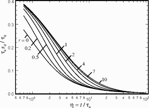
The aforementioned derivations of the sensitivity coefficients are based on the assumption that the phase front X at a given time t is a function of τt and τq with all the other parameters remaining constant. All the sensitivity coefficients are computed with a high degree of accuracy using Mathematica. Figure 1 shows the variation of τasq/τq within equation (18b)(---595--18-) as a function of r and η; that is, (---595--19) This will facilitate the prediction of sq for all values of τq and τa = τq + τtCs/C. 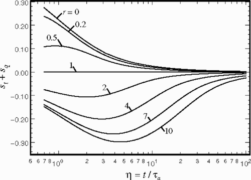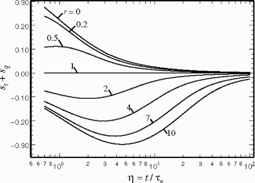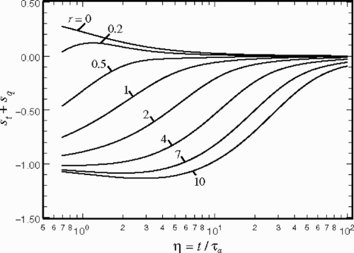In addition, equation (18a)(---595--18-) reduces to (---595--20) Figure 2 shows the variation of the function st + sq as a function of η and r. This scheme permits a graphical presentation of τt and τq without using τq/τa as a secondary variable.

Figure 1. Variation of the sensitivity coefficient sq with η and r for Case 1.

Figure 2. Variation of the sensitivity coefficient's sum with η and r for Case 1.

Figure 1 shows the sensitivity coefficient sq > 0 over the entire range of the variables η and r. Moreover, sq has a relatively larger value when η<10 and τq is finite. Figure 2 indicates that st + sq is negative when r > 1; therefore, the magnitude of |st | exceeds the values of |st + sq | plotted in figure 2 since sq > 0. Figure 2 also reveals that st + sq = 0 when r = 1. This information is significant because the variables st and sq have the same magnitude with opposite signs. This implies that these two sensitivity coefficients become linearly dependent and it will be difficult to predict both values τt and τq in the neighborhood of r ≈ 1. The analysis shows that the magnitude of st becomes small as r reduces from below 1.

When τq/τa is finite, according to equation (8)(---595--8) , it is possible to write (---595--21-) that reduces to (---595--21-) The equality in this relation serves as a limit since C includes the effect of latent heat and it is generally larger than Cs. To further elaborate on this issue, the value of st vanishes when τt = 0 and therefore τq/τa = 1. Therefore, having Cs ≠ 0, the coefficient τq/τa = 1 implies r = 0. When the τt value is small but finite, the parameter τq/τa will have a near unit value.

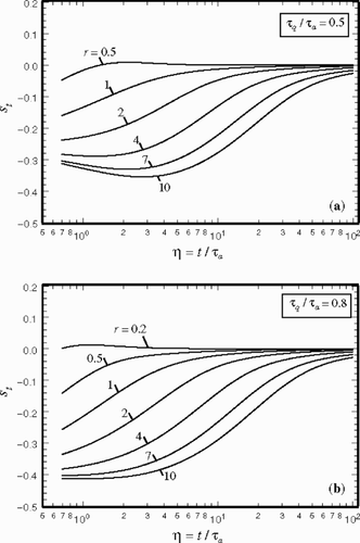
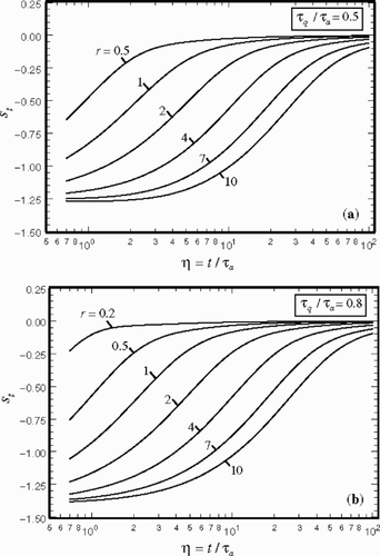
Figure 3 shows the variation of st when τq/τa = 0.5 and τq/τa = 0.8. This figure shows that the st values are small when the parameter r is small. According to equation (21b)(---595--21-) , τq/τa = 0.8, the lowest limiting value for r is 0.2 while when τq/τa = 0.5, the lower limit is r = 0.5. Moreover, according to equation (18b)(---595--18-) , as τq → 0, then sq = 0 and then figure 2 directly provides the values of st.

Figure 3. Variation of the sensitivity coefficient st with η and r when (a) τq/τa = 0.5 and (b) τq/τa = 0.8.

3.2. Case 2

This case assumes that the solid matrix arrives at a fixed temperature; that is Ts (0, t) = T0. This yields the following theoretical location of the phase front as (---595--22) Equation (22) has a form similar to that of equation (12)(---595--12) except for two modifications: the first modification replaces the factor (---595----10) by (---595----11) and the second modification is the addition of τ and (---595----12) within the integrand. Therefore, equation (13)(---595--13) is to be replaced by the following relation (---595--23) while equations (14a)(---595--14-) and (14b)(---595--14-) are to be replaced by (---595--24) that can be written as (---595--25) Finally, equations (18)(---595--18-) –(20)(---595--20) can provide the sensitivity coefficients when X* is taken from equation (22)(---595--22) , ∂X*/∂r from equation (23)(---595--23) , and ∂X*/∂η from equation (24)(---595--24) or (25)(---595--25) .

Figure 4 shows the variation of τasq/τq for Case 2 using equation (19)(---595--19) . The behavior of the sensitivity coefficient sq is similar to that for figure 1; however, its magnitude is larger. The values of sensitivity data when r = 0 remain the same for the data in both figures 1 and 4 and there is a larger dispersion when r varies between 0 and 1. The values of st + sq for this case are plotted in figure 5. Again the graph shows a slight increase in the values of st + sq in comparison to the data plotted in figure 2. A significant difference is that the data in figure 5, when r = 1, are finite. This is in contrast to those in figure 2 where st + sq = 0. There are theoretical reasons for this phenomenon. In general, when r = τt/τe = 1, equation (1)(---595--1) can be written as (---595---1) Therefore, a solution based on the assumption of local thermal equilibrium (LTE) also satisfies this equation. For Case 1, the values of Tp were prescribed at x = 0 and at t = 0; therefore, the final solution became independent of τt and τq. However, for Case 2, the temperature of the solid matrix Ts was specified at x = 0; therefore, an examination of equation (2)(---595--2) shows that the temperature Tp would depend on τt. Figure 6 demonstrates the behavior of st for two values of τq/τa = 0.5 and 0.8. The data indicate a similar trend to those in figure 3 but st values have larger magnitudes.

Figure 4. Variation of the sensitivity coefficient sq with η and rst + sq for Case 2.

Figure 5. Variation of the sum of sensitivity coefficient's st + sq with η and r for Case 2.

Figure 6. Variation of the sensitivity coefficient st with η and r when (a) τq/τa = 0.5 and (b) τq/τa = 0.8.

4. Parameter estimation using experimental data

4.1. Experimental data

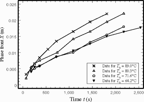
The experimental data utilized in this estimation consists of the measurement of the phase front during the melting of 99% pure tetracosane within a bed of randomly packed 3-mm diameter solid glass spheres. The commercially available glass spheres have desirable thermophysical properties and they are opaque to thermal radiation with wavelengths larger than 5 µm. The porosity of this porous medium is 0.446. The tetracosane has a melting temperature of 49.5°C. The density is 796 kg m⁻³ at and near the melting temperature and the latent heat of fusion is 255 kJ kg⁻¹. The other thermophysical properties of tetracosane are: the thermal conductivity of liquid phase is 0.17 W m K⁻¹, and the thermal conductivity of solid phase is 0.24 W m K⁻¹, both at and near the melting temperature. Using a guarded hot plate technique and steady state condition, Nnanna [7] measured the equivalent thermal conductivity of the PCM-saturated porous medium to be 0.55 W m K⁻¹. The measured locations of the phase front as a function of time are shown in figure 7. The graph includes four sets of data, each for a different surface temperature, T0 = 89.0, 80.3, 71.6, and 64.2°C.

Figure 7. Measured phase front location as a function of time for different T0.

4.2. Parameter estimation

Case 2 relates to the experimental data gathered in this study. There are three parameters to be estimated, L, τt, and τq. It is possible to determine the average value of the effective latent heat of fusion L that includes the effects of porosity and the influence of the mushy zone. A direct estimation of L is possible by examining the variation of the phase front at larger values of time when the assumption of LTE is valid. Under LTE condition [9], the following relation applies, (---595---2) According to this relation, each set of (t, X) data in figure 7 provides a value for L and the computed mean value is L = 208.9 kJ kg⁻¹. Once the value of L is known, the effective heat capacitance (---595----13) is readily available and it would depend on the surface temperature T0 while the heat capacitance of the solid matrix is a constant, Cs = 1583 kJ m⁻³.

The final task is the determination of optimum values for τt, and τq using the data in figure 7. The method of estimation, discussed below, requires initial estimations for τt, and τq. The relation (---595----14) [10] yields an initial estimated value of τq ≈ 50 s. An initial estimation for the value of τt depends on the interstitial heat transfer coefficient h [10]. For an initial estimation, τt ∼ (---595----15) when hrh /ke = 2/3 provides the interstitial heat transfer coefficient and Ts − Tm ≈ 4–5°C; this procedure yields a value of τt ≈ 60 s.

The basic estimation procedure is the method of choice [2, section 7.4] for computing τt and τq. In the following presentation, τt,e is the initial value of τt and τq, e is the initial value of τq. Moreover, X m,i is the measured value of phase front X for the i-th data while values X c,i is its computed value obtained using τt, e and τq,e in equation (22)(---595--22) . This leads to the following relations based on the Taylor series expansion [3], (---595--26) where N is the number of data points, a1 = τ t /τ t, e − 1, and a2 = τq /τq, e − 1. Since st and sq are computed at a time at which X m, i is measured, this leads to a 2 × N matrix of the sensitivity coefficients and equation (26)(---595--26) takes the form (---595--27) that can be rewritten, in shorthand notation, as (---595--28) where S is the matrix of the sensitivity coefficients, A is the vector of unknowns (a1, and a2), and D is a vector that contains the deviations. 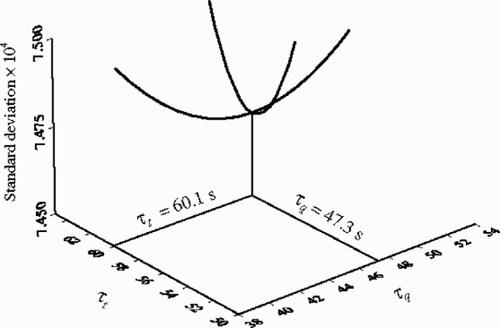The unknown coefficients a1, and a2, members of vector A, are obtainable from the relation (---595--29) Once the values of a1, and a2 are in hand, the following relations provide the new values for τt and τq, (---595--30-) and (---595--30-) The computed values of τt and τq can serve as a new set of estimates. An iterative procedure produced τt = 60.1 s, and τq = 47.3 s due to the combined effects of the surface temperature values in figure 7. These quantities resulted in a standard deviation in the estimated value of X equal to ∼0.00075 m. By definition, the standard deviation (SD) is (---595---3) and it is plotted in figure 8 to demonstrate the behavior of SD as each τt or τq deviates from the computed minimum of 0.0007474 m. Figure 8 indicates that both lines have the same minimum and the changes in the computed value of SD is small as τq changes. In contrast, a small change in τt results in an appreciable change in SD.

Figure 8. Variation of the standard deviation at and near its estimated optimum value of SD = 0.0007474 m as τt or τq changes.

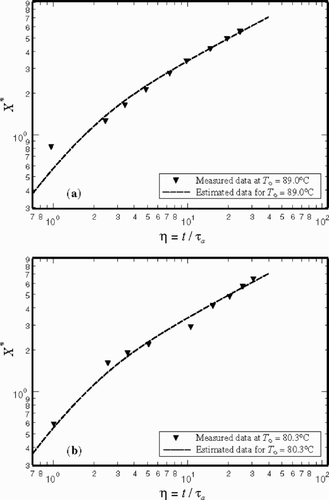
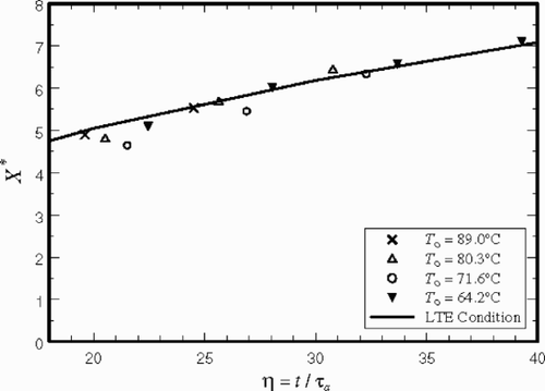
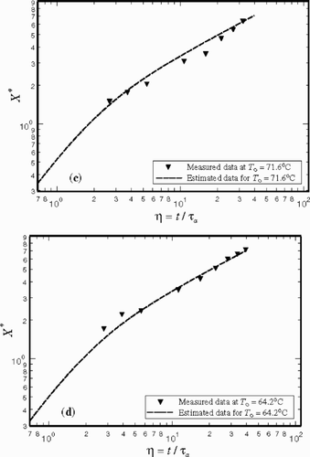
Following the determination of τt and τq, it is appropriate to demonstrate a comparison between the computed and measured values of X*. Although the data in figure 7 show significant uncertainties, the estimated phase front in figures 9(a,b) agree reasonably well with the measured values. Figure 9(c) shows larger differences while a slightly improved accuracy in the estimated values is detectable in figure 9(d). Moreover, Figure 10 shows the values of X* computed under near LTE condition when L = 208.9 kJ kg⁻¹. Figure 10 contains the data in figures 9(a–d) – at larger values of time η, as they approach the LTE condition. There is a reasonably good agreement between the asymptotic behavior of the discrete data and the theoretical solid line obtained assuming LTE condition; this attests to the accuracy of the estimated value of L.

Figure 9. A comparison of the measured and estimated values of dimensionless phase front when (a) T0 = 89.0°C, (b)T0 = 80.3°C, (c) T0 = 71.6°C, and (d) T0 = 64.2°C.

Figure 10. The behavior of experimental data at near LTE condition.

In the derivation of equation (5)(---595--5) , it is hypothesized that after initiation of the phase change process all the thermal energy entering the wall will be consumed during the phase change process; therefore, the heat flux is approximated to be independent of position at any time t. Certainly, this assumption introduces errors at two occasions: first, at the beginning of the process, since there is a rapid change in temperature near the boundary before the onset of and during the phase change process. Second, later in the process, there will be a departure from the theory because a measurable but small Ts − Tm does not produce sufficient melting and this causes a mushy zone to form and advance ahead of the phase front. However, these effects do appear if the local temperature is computed as a function of time. Based on the assumption of quasi-constant wall heat flux, (---595--31-) This approximation suggests that the solid phase temperature is a linear function of x; therefore, one can write (---595--31-) and the corresponding dimensionless temperature as (---595--31-) Accordingly, the value of θs(x, t) is readily available as the value of X(t) was defined earlier. Since (---595----16) , the relation (---595--32) yields the value of θp(ξ, η) and subsequently the mean temperature of materials in the pores Tp(x, t).

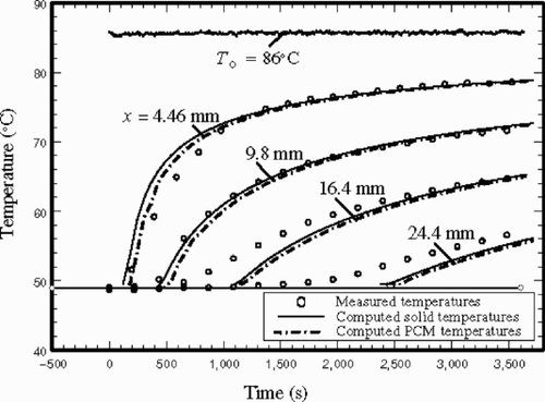
As an illustration, this procedure was employed to compute the values of Tp(x, t) using equation (3)(---595--3) and Ts(x, t) using equation (4)(---595--4) . The inverse Laplace transforms were obtained numerically by a special Mathematica [22] inversion package [23]. In addition, the analysis includes an estimated contact resistance of 0.0055 m² K W⁻¹ between Ts(0, t) and the wall. For the purpose of investigating the expected accuracy, the computed temperature is compared with an alternative set of data, different from those used in the earlier analysis. This set of data is plotted at four different locations, using discrete symbols, in figure 11. The data are for the initial temperature of 49°C and a wall temperature of ∼86°C. There is a remarkably good agreement with the recorded temperature at x = 9.8 mm. At a location closer to the wall, the experimental data show lower values at small values of time. This is due to the first uncertainty case, discussed earlier, because the analysis ignores the capacitance of the porous materials. This situation is reversed at the locations further away from the surface, as the experimental data have higher values at smaller relative time. This implies that the mushy zone may have extended to beyond the theoretical prediction of the location of the phase front. According to data plotted in figure 11, the temperature deviation is ±4°C indicating a reasonable error of ±11% in the computed values of heat flux from the wall. This error is consistent with the deviations detectable in figures 9 and 10 in the estimation of the location of the phase front.

Figure 11. A comparison of the predicted temperature with the experimentally acquired data when T0 = 86°C.

5. Conclusion

Results for the first case show that for any given ratio τt/τq, the sensitivity coefficient decreases asymptotically to zero at large times. Furthermore, the sum of the sensitivity coefficients is st + sq = 0 when τt/τq ≈ 1. This information is significant because the variables st and sq have the same magnitude with opposite signs. This implies that these two sensitivity coefficients become linearly dependent and it will be difficult to predict the values of τt and τq in the neighborhood of τt/τq ≈ 1. A similar trend but with different sensitivity values is reported for the second case.

This study reveals that the problem of rapid melting/freezing of a porous material differs from that under LTE condition. The procedure employed is an effective method to study the local thermal non-equilibrium behavior of phase change materials. The earlier data show that during the melting of materials in a cell, there is a measurable temperature difference, Ts − Tp, that can exceed 4°C. This difference gradually disappears upon termination of the phase change process. In general, this study shows that the theoretical model in [9] adequately predicts the location of the phase front. However, the temperature predictions are accurate when the mushy zone is small. Figure 11 shows that the agreement between predicted and measured local temperature improves following the completion of melting and disappearance of the mushy zone.

Nomenclature

Table

A=	surface area, m^2
A=	correction vector for coefficients
C=	(---595----17) , J m^−3 K^−1
(---595----18) =	mean heat capacitance of materials in pores, J m^−3 K^−1
Cs=	solid heat capacitance, J m^−3 K^−1
D=	deviation vector
ke=	effective thermal conductivity, W m^−1 K^−1
L=	latent heat of fusion, J kg^−1
LTE=	local thermal equilibrium
LTNE=	local thermal non-equilibrium
r=	τ t/τ a
rh=	hydraulic radius
Rc=	contact resistance, m^2 K W^−1
r=	position vector, m
sq=	dimensionless sensitivity coefficient for τq
st=	dimensionless sensitivity coefficient for τt
S=	sensitivity matrix
t=	time, s
Tm=	phase change temperature, K
T0=	surface temperature at x = 0, K
Tp=	mean temperature of pore materials, K
Ts=	solid matrix temperature, K
x, y, z=	coordinates, m
X=	location of the front, m
X*=	(---595----19)
V=	volume, m^3

Greek symbols

Table

α=	thermal diffusivity, ke/C, m^2 s^−1
βq=	∂X/∂τq
βt=	∂X/∂τt
ε=	Vf /V
η=	t/τa
θp=	(---595----20)
θs=	(---595----21)
ξ=	(---595----22)
ρ=	density, kg m^−3
τ=	dummy variable
τa=	(---595----23)
τe=	Cs τt /C
τq=	lag time in heat flux, s
τt=	lag time in temperature, s

Subscripts

Table

c=	contact
e=	equivalent
p=	pore
s=	solid