Material constants identification in anisotropic materials using boundary element techniques

Abstract

This article addresses the resolution of the inverse problem for parameter identification in anisotropic materials. It is based on Boundary Element techniques and it is approached as an optimization problem of a residual cost functional. For this purpose, a standard non-linear minimization method, the Levenberg–Marquardt algorithm, is used. This algorithm makes use of the functional derivatives with respect to the material constants, which in this article have been calculated using direct differentiation procedures. The formulation is developed for plane problems that are in general anisotropic, for homogeneous or piece-wise homogeneous domains. Several examples have been carried out in order to prove the validity of the proposed procedure. The numerical results presented demonstrate the effectiveness of the method employed.

Keywords:

• Inverse problem
• Parameter identification
• Material constant identification
• Two-dimensional anisotropic elasticity
• Boundary element method
• 31A25
• 74B05

1. Introduction

The use of anisotropic materials is more and more common in the fabrication of high-performance structural systems lately employed in the aeronautical, architectonic or aerospace fields. Hence the importance of knowing accurately the material properties in order to predict, in a precise way, the behavior of the structure. The material constants can be identified from laboratory experiments based on either static or dynamic response to external excitations. Nevertheless, sometimes, the values determined from standard laboratory tests may differ significantly from the actual ones, when the components are manufactured in the factory. In other cases, the material sample cannot be tested, thereby in situ Non Destructive Evaluation (NDE) techniques are needed. The deduction of the elastic properties of a non-isotropic elastic solid from its response may be formulated as an Inverse Problem (IP). Direct (or Forward) problems are those where the response of the system can be determined, provided that the geometry, the governing equation, material properties and the boundary conditions are given. On the contrary, in IPs, some of this information is unknown, and this is compensated with extra information obtained from the system response. Inverse problems are an important topic of research, and have been extensively studied in recent years. In general, IPs are ill-posed and unstable against small errors in the measurements; therefore a suitable algorithm must be chosen in order to solve them. The most common approach makes use of minimization techniques, together with modeling techniques such as Finite Element Methods (FEMs) and Boundary Element Methods (BEMs).

While there is a vast literature presenting theoretical results about the IP of impedance tomography (see for instance [1–4] and references therein), the corresponding elastic problem has received much less attention. Nevertheless, important theoretical results have been obtained by some researchers: Ikehata [5] has shown that the Lamé constants of an isotropic elastic body can be determined by the Dirichlet-to-Neumann data map. Lin [6] proved that the radially dependent Lamé coefficients of an isotropic spherical body can be obtained by making only two measurements of displacements and stresses on the body surface. Some of these results were extended to two-dimensional anisotropic bodies by Ikehata [7,8] and Nakamura et al. [9,10] using the Dirichtlet-to-Neumann map.

There are many computational studies with the aim of determining the elastic constants of a body from boundary data, but mainly for isotropic bodies. Schnur and Zabaras [11] have determined the size and location of a circular inclusion within a finite plate matrix, together with the isotropic elastic constants of the inclusion and matrix. They make use of FEM and the Levenberg–Marquardt method to minimize the difference between the response of the system and the model.

Mallardo and Alessandri [12] applied Boundary Element techniques to a very similar problem, but in this case the gradient of the functional was computed by implicit derivation, instead of the finite differences used in [11].

Constantinescu [13] has treated the identification of material properties and defects in composites by minimizing the error of the constitutive law, within the elastic impedance tomography framework.

Heyliger et al. [14] used a dynamic method based on the measurements of the free vibrations in three-dimensional anisotropic bodies excited by impact resonance.

Wang and Kam [15] proposed a constrained minimization method for determining the elastic constants of shear deformable composite materials. Also the material properties of composite plates have been identified by Liu et al. [16] where they combined a genetic algorithm with non-linear least squares techniques.

Recently, Marin et al. [17] retrieved the isotropic material constants with minimization techniques from boundary measurements only. Finally, Lauwagie et al. [18] proposed a mixed numerical–experimental method to determine the in-plane elastic properties of orthotropic plates.

In this article a formulation for identifying the elastic constants of a rectilinearly anisotropic two-dimensional material is presented. The method combines a Boundary Integral Equation formulation with a least-squares technique. It consists of the minimization of a cost function, the square sum of the differences between boundary measurements and computed values of displacements/tractions. The Levenberg–Marquardt algorithm has been used, which implies the computation of the cost function derivatives with respect to the unknown material constants. The finite-difference Jacobian matrix has been extensively used by many authors [19]. Instead, in this work we use explicit expressions of the boundary displacement/traction derivatives with respect to the elastic constants, thus the computational effort is reduced. For the numerical implementation, isoparametric quadratic boundary elements are employed. The domain can be finite or infinite, homogeneous or piece-wise homogeneous. A series of applications is presented and the method proposed validated.

2. Boundary Element Method for anisotropic materials

We consider the elastostatic equilibrium of a homogeneous solid Ω having general anisotropy, whose surface is denoted by Γ. Boundary conditions are prescribed on the whole boundary and can be of any type, Dirichlet, Neumann or mixed; zero body forces are assumed. The geometry and boundary conditions model a pure plane strain state; hence magnitudes of the problem (displacements, stresses and strains) can be simplified to a two-dimensional study. The problem is governed by the equations (---635--1) plus the boundary conditions. The vector u represents the displacement vector, whilst the symmetric tensor σ is the stress tensor at any point x ∈ Ω. The strain tensor, defined by, (---635--2) is related to the stress tensor by Hooke's law, (---635--3) where a is the elastic constant tensor.

For the anisotropic two-dimensional case, if the middle plane of the body is taken as the coordinate plane 1–2, Hooke's law can be expressed as (---635--4) where the two-index notation for stresses and strains has been transformed to a one-index notation: 11 → 1, 22 → 2, 12 → 6.

The analytical solution of the anisotropic elastic problem defined in (1)(---635--1) plus the boundary conditions, can be found for a limited number of cases, only when the geometry and loading conditions are very simple. To solve more realistic problems one needs to resort to numerical approaches. The BEM is a family of methods based on Boundary Integral representations of the displacements and/or tractions on the boundary: in this article a collocation approach is employed. An approximate solution can be obtained with this numerical procedure for problems over finite or infinite domains, and very general geometries and boundary conditions.

This technique starts by establishing the Betti's Reciprocity theorem between two balanced systems of body and boundary forces: the actual system of the case under study, and a particular auxiliary field known as the Fundamental Solution. If z prime; is a point inside the domain Ω with boundary Γ, and assuming no body forces b, the Somigliana identity is obtained, (---635--5) where the displacement and traction fields are ui and tj for the actual problem, and Uij and Tij for the Fundamental Solution. Then, performing the limit to the boundary z′ → y ∈Γ, one obtains the Boundary Integral Equation, which governs the displacement field on the boundary, (---635--6) The free term, cijy, depends on the location of the collocation point y on smooth or non-smooth parts of Γ. In particular, cij (y)= (1/2) δ ij if Γ is smooth, where δ ij is the Kronecker delta tensor [20].

2.1. Anisotropic Fundamental Solution

The Fundamental Solution is the response at a point z, due to a point load applied at z′, in an infinite domain with the same material properties as the original problem. The solution is obtained by the complex potential approach more extensively developed in [21,22].

Briefly, if the body forces stem from a potential U, the problem can be expressed in terms of a stress function F(x1,x2) [21]: (---635--7) Then, taking into account the constitutive law and the relationship between displacements and strains, we obtain the differential equation satisfied by the function F: (---635--8) where the differential operator L4 is given by, (---635--9) This operator can be factored solving the characteristic fourth-degree polynomial equation l4(μ) = 0, (---635--10) which always has four complex roots μi, two conjugate pairs called complex parameters. It can be shown that l4(k) > 0 ∀ k ∈ R [21], and therefore l4 has no real roots; βij are termed the reduced elastic constants: (---635--11)

The stress function F is found in the form: (---635--12) where Fi(zi) are two arbitrary analytical functions of the complex variables zi = x1 + μi x2, and F0 is a particular solution of (8)(---635--8) .

To obtain the response of an infinite body when a unitary load is applied in xi direction at point z′, new complex potentials Φi are introduced such that, (---635----1) . For these load conditions and geometry the potentials Φi are given by [22] (---635--13) where Aij are complex constants found by solving the system, (---635--14) and (---635--15)

All the equations above are also valid in a generalized plane stress state, simply replacing the reduced elastic constants βij by the elastic constants aij.

Taking into account the relationships between the potentials and stresses, strains and displacements, the following displacements and tractions of the fundamental solution are found, (---635--16) and (---635--17) where q1k = μk, q2k = -1, and ni are the components of the outward normal to the boundary.

2.2. Discretization of the Boundary Integral Equation

Following a collocation BEM in order to solve equation (6)(---635--6) numerically, the boundary Γ is discretized in a number of elements Ne. The geometry, displacements and tractions are interpolated on those elements with their values at the element nodes and with some shape functions. For the present study, isoparametric quadratic elements have been employed. After discretization, the Boundary Integral equation (6)(---635--6) , written for a collocation point y^l, takes the form, (---635--18) where (---635----2) , (---635----3) , called integration constants (i = 1, 2, j = 1, 2, m = 1,2,3), are given by (---635--19) (---635--20) J^k(ξ) represents the Jacobian of the transformation to the natural coordinate in the integration element.

Evaluation of these integrals implies distinguishing between regular and singular cases, depending on whether the collocation point y^l belongs to the integration element or not. Although in the singular case improper integrals and Cauchy principal values arise, after some manipulations all of them can be numerically performed by Gaussian quadrature [20]. For detailed development of integration constants evaluation see [23].

Then, if (18)(---635--18) is collocated at every boundary node, an algebraic system of equations is obtained: (---635--21) where the vectors u and t comprise the displacements and tractions at all the nodes of the boundary, respectively. After applying boundary conditions the final square and non-singular system of equations to be solved is (---635--22) where x encompasses the unknown displacements and tractions on the boundary.

3. Inverse problem for identification of elastic material properties

The elastostatic problem stated in (1)(---635--1) is a well-posed problem if the governing equation is defined, the material properties are known and the boundary conditions are prescribed along the whole boundary. In this article we are dealing with an anisotropic elastostatic problem where the elastic constants aij are (totally or partially) unknown. In order to obtain a solvable problem, extra information has to be provided to make up for the unknown material properties. The ensuing problem is a parameter identification problem or material constant inverse problem. In practice, this extra information will be obtained through measurements on a reachable surface of displacements, strains or stresses.

The usual approach for solving the problem is to minimize an objective function, which represents the distance between the measured values and the computed ones in an assumed model.

3.1. Minimization algorithm

We are attempting to fit the measured values of a physical magnitude yi, (i=1,…, m) with their values predicted by a model, mi(x), which depend on some unknown parameters xj, (j=1, … \comma;n) (the elastic constants in our case). The measurements can be either displacements and/or tractions, which are the system response to some given boundary conditions. If we denote by f the function to be minimized, the minimization problem is defined as follows (---635--23) where R is the vector of residuals, computed as the difference between the experimental data and the values predicted by the model, i.e., Ri(x) = mi(x)−yi.

Since the model is nonlinear in x, a nonlinear least-squares problem arises. To solve it, we employ the Levenberg–Marquardt algorithm, which has been found to be advantageous in similar problems [24].

This method is quickly q-linearly convergent in problems with small residuals and not too nonlinear. It also has the advantage of being well-defined even when the Jacobian does not have full column rank, and the step is close to being in the steepest-descent direction [25].

The algorithm proceeds as follows: given an estimate xk, an affine model Mk of R^k(x) is computed, (---635--24) where Jk is the Jacobian matrix given by the derivatives, (---635--25)

Then, the original minimization problem is reduced to, (---635--26) where the restriction is established to avoid steps out of the region where the affine model is valid. The solution of the problem above provides an updated estimate of the parameters, (---635--27) where α^k is a parameter, which depends on δk.

Note that no constraint has been considered in the original minimization problem (23)(---635--23) . However, for real materials the characteristic polynomial equation (10)(---635--10) cannot have real roots [21]. Therefore after each update of the material constants, the complex parameters μi are computed and the inequalities Im(μi)≠ 0 are checked. Actually the algorithm has never reached an estimate of the material constants, such that these inequalities were violated, so they have not been enforced explicitly.

Several stopping criteria have been implemented for the Levenberg–Marquardt algorithm, such as a minimum (normalized) objective function (f(x)≤ ε1), minimum step values ((---635----4) ) and (normalized) gradient convergence ((---635----5) ), where εi = 10^-5 for all criteria. A maximum number of 100 iterations is accepted.

3.2. Sensitivity analysis

In order to obtain the Jacobian of the residual vector (25)(---635--25) , the derivative of boundary displacements and tractions with respect to the material constants has to be computed. Several approaches can be used. Instead of finite differences, which would be too expensive computationally, we opt to differentiate analytically the Boundary Integral representation given by equation (6)(---635--6) . Carrying out the derivative with respect to an arbitrary material constant apq, the following equation is obtained: (---635--28)

In this equation, besides the standard kernels Uij and Tij, two new kernels arise, namely their derivatives with respect to the compliance coefficient apq. It is important to point out that the singularity orders of the new kernels are equal to those of the standard ones. Thus, (∂ Tij(z,y)/∂ apq) is singular, while (∂ Uij(z,y)/∂ apq) is weakly (logarithmic) singular.

Discretization of the above sensitivity equation leads to, (---635--29) where, for the sake of simplicity, we have called (---635--30)

The new integration constants (---635----6) and (---635----7) are given by, (---635--31) (---635--32)

Then, if (29)(---635--29) is established at every boundary node, a new algebraic system of equations is obtained: (---635--33) that, after rearranging columns according to the boundary conditions, we get, (---635--34) where δx is a vector, which comprises the unknown derivatives of boundary displacements and tractions with respect to the material property apq. Note that δ ui = 0 at nodes where ui is given (Dirichlet boundary condition) whilst δ ti = 0 where ti is given; consequently, the system matrix A, is the same as for the direct problem shown in equation (22)(---635--22) .

Issues about the computation of the new integration constants (---635----8) and (---635----9) and more details of the differentiation process can be found in [23].

3.3. Uniqueness and stability of the determination of elastic constants from boundary data

The elastic constants of an anisotropic body, or a subregion within it, are not uniquely determined for any loading conditions and support. First of all, it is obvious that in regions of the domain where the stresses were zero, any distribution of elastic constants would produce the same distribution of displacements and tractions on the boundary. Moreover, if one component of the stress tensor is zero, say σ12, the corresponding elastic constant in the diagonal of matrix a, (a66 in this case) will be undetermined. This problem will not appear as far as the region whose elastic constant we are trying to obtain is under a general state of stresses, which is not zero nor very small throughout the region of interest.

Secondly, a given uniform distribution of stresses may lead to the same distribution of strains, and therefore the same displacements on the boundary, for different elastic constants. To show this fact, consider a uniform stress field σj and the corresponding strain field ϵi such that (4)(---635--4) , (---635--35) for a given set of elastic constant. A perturbed set of elastic constants (---635----10) will yield the strains, (---635--36) for the same stress field. The strain fields will fulfill the equation (---635----11) provided that, (---635--37) Then, any perturbation (---635----12) of the elastic constant matrix, such that the given tensor σj belongs to its kernel will not change the strain field. Therefore, if the cost functional involves only displacement measurements, and the stress field is approximately constant, then there will be multiple solutions for the material property inverse problem, since for any stress field vector σj there exists a symmetric matrix (---635----13) such that (---635----14) . For instance, an arbitrary stress field tensor σ 11= α, σ 22= β, σ 12= γ, belongs to the kernel of the matrix, (---635--38)

Thirdly, in cases where the loading and boundary conditions are such that the direct problem is isostatic (statically determined), the stress field, by definition, will be insensitive to changes in the elastic constants. Obviously, in this case, an inverse problem based on a cost functional that involves only tractions on the boundary will have multiple solutions.

In order to avoid the above-mentioned situations, the loading and boundary conditions and the boundary measurements should be properly designed. Firstly, the stress field should be general, that is, all components should have a non-zero value. Secondly, the cost functional should involve both displacements and tractions on the boundary, if necessary. Thirdly, the stress field should be variable and as sensitive to changes in the elastic constants as possible, i.e., as statically undetermined as possible. Finally, the number of material constants to determine can be reduced, in order to preclude the existence of perturbations (---635----15) such that (---635----16) .

Nevertheless, designing an IP such that all six elastic constants can be obtained from a unique experiment is not easy, even if the conditions stated in the paragraph above are fulfilled, since the cost functional will be much more dependent on some elastic constants than on others, as shown in the applications below.

4. Numerical applications

4.1. Tests definition

To prove the effectiveness of the proposed approach for the identification of the material properties, three cases have been studied. The first and second are homogeneous square plates composed of just one material with anisotropic elastic properties. Both cases differ in the load conditions acting on the plates. The values of the six elastic constants, where the index 1 denotes the horizontal axis while the index 2 denotes the vertical direction, are detailed below (in (m2(GN)^-1)), (---635--39)

The third case consists of a square plate with an internal inclusion made of a different material. The material properties of the inclusion will be the ones to be identified, and their exact values are the same as (39)(---635--39) . The elastic constants of the material outside the inclusion are considered known and their values are given by (in (m2(GN)^-1)), (---635---1)

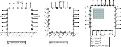
The outer boundary of the plate in the three cases has been modeled with 24 isoparametric quadratic elements. In the third case, the inclusion is meshed by 24 elements. Displacements on the boundary are measured at several locations; 18 in case 1 and 20 in cases 2 and 3. Actually, these measurements are simulated computing with the BE code the displacements at the chosen locations using the exact elastic constants we are looking for. To avoid the so-called inverse crime, Gaussian noise has been added to these simulated data. The geometry, boundary conditions and measurement locations are shown in figure 1 for each case.

Figure 1. Geometry and load conditions, cases 1–3.

4.2. Results

Two different types of tests have been run. In the first one, we have considered no error in the simulated experimental data. Then, to check the stability of the proposed method, the data is perturbed with small errors. Therefore, in the second group of tests, a specific percentage of Gaussian noise is added into the simulated measurements.

4.2.1. Exact data tests

The six elastic constants are considered unknown and must be identified. Three initial guesses have been tested, each of them differs in a certain percentage from the real values, 50, 100 and 400%, respectively. Figures 2–4 show the evolution of the cost function versus the iteration number. Below each graph, there is a table with the initial elastic constants and their values achieved at the last iteration.

Figure 2. Cost Function minimization with exact experimental data in case 1.

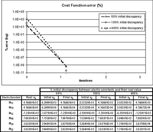
Figure 3. Cost Function minimization with exact experimental data in case 2.

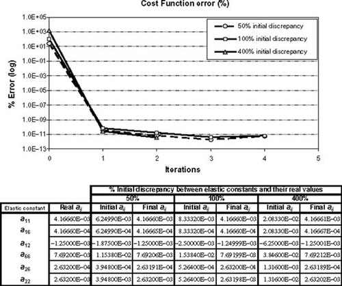
Figure 4. Cost Function minimization with exact experimental data in case 3.

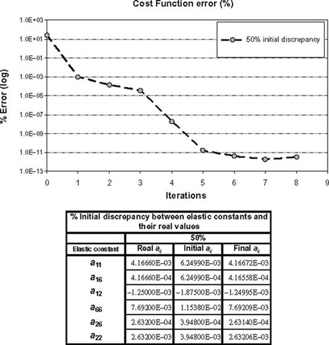
It can be seen that in all cases, the convergence of the elastic constants to their exact values is very good. These are cases in which stresses are not sensitive to small variations in elastic constants, and therefore the relationship between the cost function and the material properties is nearly quadratic. This implies that the minimum is reached in one or just a few iterations. In the third example (see figure 4) the convergence is attained when the initial estimate is not very far from the exact values (50%). In other cases, the existence of local minima precludes the convergence to the exact values.

4.2.2 Noisy data tests

In practical situations, it is impossible to get exact experimental data when measuring physical quantities. Besides, the numerical model never represents exactly the behavior of the real specimen. Therefore, when solving inverse problems, one very important aspect to be studied is the effect that errors introduced in the measurements can cause in the resolution process. The next figures show some examples where the simulated measurements, computed with the exact material constants, have been modified introducing several percentages of error, 2 and 5% (following a Gaussian distribution).

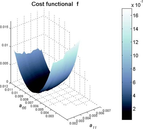
The identification of four parameters for case 1 and two for case 2 is plotted in figures 5 and 6, with 2 and 5% error in measurements. Figure 7 shows four different runs in which 2% random error is introduced in case 3. In all four cases, three elastic constants have been successfully predicted. The minimization process with noisy data becomes much more complicated since the cost function has local minima. The non-linearity of this objective function produces situations in which specimens with different material properties may have very similar stress/strain distributions. Figure 8 illustrates the cost function surface when the values of a11 and a66 vary (±50% of their true value), for case 3. A 2% error has been introduced in the experimental data. Note that the cost function is much more sensitive to changes in a66 than in a11, and therefore the minimum is difficult to attain.

Figure 5. Cost Function minimization with 2% (left) and 5% (right) random error in experimental data for case 1.

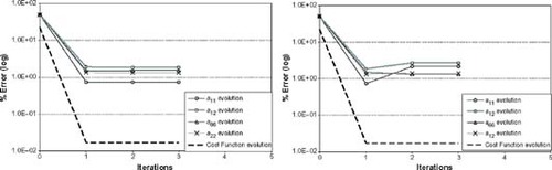
Figure 6. Cost Function minimization with 2% (left) and 5% (right) random error in experimental data for case 2.

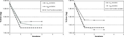
Figure 7. Cost Function minimization with 2% random error in experimental data for case 3, four different runs.

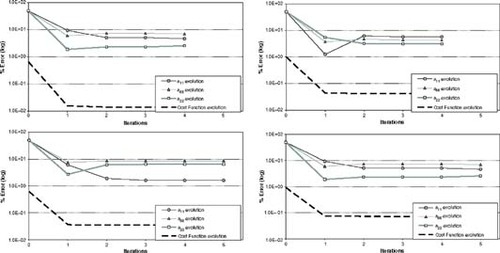
Figure 8. Cost Function minimum surface with 2% error in experimental data in case 3 for variations in a11 and a66.

5. Conclusions

In this article, we investigate the identification of the material properties corresponding to a two-dimensional anisotropic linear elastic medium. The proposed approach combines a BEM and a minimization algorithm. In particular, the Levenberg–Marquardt algorithm has been chosen. When using this technique, derivatives of displacements and tractions on the boundary with respect to the material constants must be computed. These derivatives are obtained from the material constant derivative Boundary Integral Equation which is computed analytically and discretized following standard BE techniques. Several tests have been performed to investigate the convergence of the algorithm. Different aspects, such as number of measurements, noise in data, initial guess values and number of iterations have been taken into account. Overall, it is concluded that the proposed iterative approach produces an accurate, convergent and stable numerical solution to this particular inverse problem.