Abstract
This article presents experimental results of local thermal boundary conditions obtained by solving the inverse heat conduction problem. The experimental study concerns the heat transfer of a liquid film falling on a horizontal tube. The test fluid is water. An electric resistance heater is placed inside the tube. The thermocouples are installed in order to measure the temperature in the solid. The flow rate of the liquid film is varied. The iterative regularization method is used to solve the inverse problem under study. The unknown functions are approximated by cubic B-splines. The gradient is computed by using the adjoint equations. This article shows the application of an inverse analysis to determine the local thermal boundary characteristics when measurements are difficult without perturbing the flow.
1. Introduction
Falling liquid film heat exchangers have been in use for a long time in the heat transfer industry because they provide high heat transfer coefficients at low flow rates and reduced temperature differences. Falling film evaporation and condensation on a horizontal tube has been used in the chemical, refrigeration, petroleum refining, desalination and food industries Citation[1,Citation2] for many years.
When a liquid film falls from a horizontal tube to another horizontal tube placed below, different flow modes, such as the droplet regime, droplet and column mixed regime, columns, column and sheet mixed mode, and the sheet regimes are observed depending on the flow rate. Several experimental and theoretical studies on the heat transfer and hydrodynamics of falling liquid film on horizontal tubes have been reported in the literature Citation[3–Citation6]. Numerous studies are conducted to evaluate the average heat transfer coefficients, but the estimation of the local heat transfer without neglecting the heat conduction in the solid has not retained much attention.
The study of the heat exchange requires the knowledge of the thermal boundary conditions, such as the local surface heat flux, the local surface temperatures or the local heat transfer coefficients. The inverse heat conduction problem (IHCP) has been used to analyze the physical phenomena where direct measurements are difficult or impossible to carry out. Various numerical algorithms have been proposed Citation[7–Citation13].
In this work, the IHCP is applied to the problem of a hollow cylinder heated at the internal surface. The iterative regularization method is used to solve the inverse problem under analysis. This method was chosen because it can easily be extended for nonlinear inverse problems. The method is based on the conjugate gradient method to minimize the residual functional and the residual discrepancy principle as the regularizing stopping criterion.
This article presents the experimental study of natural heat transfer of falling film on a horizontal cylinder. The numerical algorithm developed to solve the IHCP is described. The experimental results of average heat transfer coefficients are compared to the estimated results using IHCP. The influence of the sensors position and temperature measurement errors are discussed.
2. Experimental setup
The test facility shown in is composed of two circuits. The first one is a closed circuit where the test liquid is in forced circulation. The fluid is delivered through a liquid pump (3) from the reservoir (2) to the adjustable constant head tank (5) equipped with a drain and an overflow. A filter is used to eliminate any dust or particles in the working fluid. An electrical heater associated with a temperature controller is installed in the head tank (5) to control the temperature of the test liquid (8). A Chromel–Alumel thermocouple is installed in the liquid bath to measure the temperature of the fluid in order to estimate the liquid properties. The second circuit consists of the feed to the test section. The fluid from the overhead tank flows under gravity through the flow meters and the regulating valves to the interior of the tube Equation(12)(12) placed at the top in the test section.
Figure 1. Experimental setup.
shows the disposition of the tubes in the test section. Following Mitrovic's method Citation[14] 202 holes of 1 mm diameter 1.5 mm apart are drilled on the bottom of the upper feed tube having an inside diameter of 16 mm and outside diameter of 18 mm. The gap between the bottom of the first tube and the top of the second tube of the same diameter used for the flow distribution is 1.4 mm. The working fluid delivered through holes in the first tube flows on the outside surface of the second tube to give a uniform distribution of the flow along the lower test cylinder and then drops in the reservoir. A 19-mm gap is used between the bottom of the second tube and the top of the test cylinder of outside diameter 50 mm and length 140 mm. The described test setup has been realized to study falling film evaporation heat transfer with different liquid flow patterns. The flow rate is adjusted through two needle valves placed at the extremities of the feed tube. Two flow meters are installed to measure the liquid flow rate.
Figure 2. Disposition of tubes in the test section; Ø: diameter.
The experimental section shown in is made of transparent plastic (polycarbonate) and has a rectangular cross section of 90 × 500 mm2. Two vertical sides of the test section are used to support the tubes. The front cover of the test section is removable and allows to measure the flow rate of the liquid downstream of the experimental copper cylinder by determining the weight of the liquid collected during a known period of time.
Figure 3. Photo of the test section.
shows schematically the flow of a liquid film on a cylinder. Determination of the local heat flux in such a case when the surface is covered with liquid of variable thickness as is usually the case for single-phase and two-phase flow process is a difficult problem. The thickness of the liquid film is generally less than 500 µm and it is difficult to measure directly the velocity and temperature distributions in the flowing film. Only the bulk temperatures at the inlet and outlet and the wall temperatures are easily accessible.
Figure 4. Liquid film flowing around a horizontal cylinder.
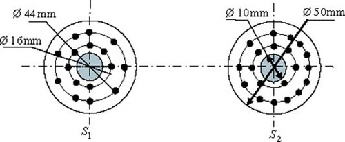
Because of the uncertainty in the heat flux distribution along the length of the cylinder, the wall temperature distribution was measured at two different sections as shown in . The temperature is measured inside the test cylinder with the thermocouples (type K) placed at 3 and 9 mm from the wetted surface (see ). Thus the temperatures for two radii along a radial line were measured for a given angular position using 37 thermocouples. For the section S1 nine thermocouples are used at 3 mm from the outer surface at intervals of 22.5° on one half of the cylinder and four thermocouples are located at intervals of 45° on the other half of the cylinder. For the section S2, five thermocouples are placed at 3 mm from the outer surface at intervals of 45° on one half of the cylinder but on the other half of the cylinder, two thermocouples are located at intervals of 22.5° and two other thermocouples are installed at intervals of 45°. For each section, eight thermocouples are located at a distance of 17 mm from the outer surface at intervals of 45°.
Figure 5. Location of the measurement sections.
A data acquisition system is used to record all temperature measurements for each imposed electric power at internal radius of cylinder. The IHCP is solved to determine the local heat flux and the surface temperature of the heated tube. The local heat transfer coefficient is determined around the experimental tube for different flow rates. The experiments are conducted for inlet liquid film temperature of 30°C and the total electric power imposed at the internal radius of 320 W. For each flow rate, the measured temperature inside the wall of the experimental tube is used to solve the IHCP in order to determine the thermal boundary conditions of a falling liquid film on the horizontal tube.
3. Inverse problem
The physical model considers an infinitely long cylinder of internal radius R1 and external radius R2 (). The temperatures at the radius R1 are imposed. The solution of the inverse problem is carried out for half of the cylinder. The mathematical model of a heat conduction process in a hollow cylinder treats the steady-state heat transfer problem. It is given by the following system of equations:
(1)
where, R1<r<R2, Φ1<ϕ<Φ2,
(2)
(3)
(4)
(5)
The mathematical model is supposed to be symmetrical about the vertical axis of symmetry (Φ1 = 0, Φ2 = π).
Figure 6. Location of the thermocouples in the solid; Ø: diameter.
In the inverse problem, the heat flux Qw(ϕ) at the external surface of the cylinder is unknown. The temperatures measured at nodes (rn, ϕn) inside the solid are used as an additional information on the temperature distribution in the cylinder to estimate the function Qw(ϕ):
(6)
The IHCP consists in estimating the function Qw(ϕ) using the conditions Equation(1)
(1) –Equation(6)
(6) .
The solution of the inverse problem is based on the minimization of the residual functional defined as:
(7)
where T(rn, ϕn; Qw) are the temperatures at the sensor locations computed from the direct problem Equation(1)
(1) –Equation(1)
(1) –Equation(5)
(5) .
The unknown heat flux is approximated in the form of a cubic B-spline as follows:
(8)
where m is the number of approximation parameters, pi are the unknown approximation parameters and ϕi are the given basis cubic B-spline. Therefore, the IHCP is reduced to the estimation of a vector of parameters p = [ p1, p2, …, pm]. The procedure and the algorithm adopted for solving IHCP is presented in Citation[15] and the details will not be repeated here. The conjugate gradient method is used in order to minimize the residual functional. The unknown function Qw(ϕ) is supposed to be an element of the L2 [Φ1, Φ2] space.
The conjugate gradient algorithm is iterative. At each iteration, the successive improvements of desired parameters are built as follows:
(9)
where ‘it’ is an iteration number. γit is the descent parameter. d it is the descent direction determined by the following expression:
(10)
where the parameter βit is computed as follows:
(11)
where ⟨, ⟩ is the scalar product, ‖;·‖; is the norm and β0 = 0.
To implement the iterative minimization procedure, the vector g is determined by the following equation:
(12)
where G is the Gram's matrix for basis functions.
(13)
⟨ ϕi, ϕj ⟩ is the scalar product in the L2 space. The Gram's matrix is symmetric and positive. Let J′(p) be the vector gradient of the functional J(p) defined as:
(14)
where ψ is the adjoint problem solution.
3.1. Descent parameter
To compute the descent parameter, the linear approximation of the descent parameter is used Citation[16]:
(15)
where θit (rn, ϕn; δQw) is computed from the problem in variations at the ‘it’ iteration by using the variation of the unknown heat flux (δQw). θit (rn, ϕn; δQw) is defined at the sensor locations (rn, ϕn). δQw is approximated from a cubic B-spline as follows:
(16)
The problem in variations is defined by the following equations:
(17)
where, R1<r<R2, Φ1<ϕ<Φ2
(18)
(19)
(20)
(21)
3.2. Adjoint problem
The necessary conditions of optimization Citation[15] are defined in the form of an adjoint problem, which is represented by the following boundary-value problem:
(22)
where,
(-1)
(23)
(24)
(25)
(26)
The gradient of the residual functional is determined by solving the adjoint problem. The symbol δ(r, rn; ϕ, ϕn) represents the Dirac function. The direct problem, the adjoint problem and the problem in variations are solved using a finite difference implicit approximation and a Gauss–Seidel procedure Citation[17] for the solution of the resulting system of linear algebraic equations.
3.3. Regularization
The inverse problem is ill-posed and the numerical results depend on the fluctuations occurring at the measurements. To obtain a stable solution of the IHCP the iterative regularization method is used by stopping iterations at the optimal value of the residual functional, which satisfies the following condition:
(27)
where δ2 is the total measurement errors defined as follows:
(28)
σ2(rn, ϕn) is the standard deviation of measurement errors for the temperatures measured at the position (rn, ϕn).
4. Experimental data processing
The numerical procedure was validated by using the temperature data obtained from the direct problem to simulate the measured temperatures inside the cylinder. The local heat flux required to solve the direct problem is known at the surface of the cylinder. The calculations were carried out using different numbers of approximation parameters Citation[18].
4.1. Determination of the local thermal boundary conditions
A horizontal copper tube (λ = 389 W m−1K−1) having the radii R1 = 8 mm and R2 = 25 mm is considered. A grid of 30 nodes along the circumference and 15 nodes in the radial direction have been used. The local thermal characteristics are computed by solving IHCP where the temperatures measured at radius R1 are used as the boundary condition to solve the direct problem because the electric heat flux distribution in the internal cylinder is nonuniform and unknown. The temperatures measured at radius Rmeas = 22 mm are used to solve the inverse problem. The computation is conducted by using the number of measurement points equal to the nodes number.
and show the estimation of the local heat flux and the surface temperature around the test cylinder. In this experiment the flow rate of falling film is 0.283 kg m−1s−1. presents the local temperature residuals resulting from this computation. The estimated standard deviation of temperature residuals of this computation is 0.04°C. The average value of the temperature residuals is about zero. shows that the residual functional decreases when the iteration index increases and reaches an asymptotic value. It is noted that heat transfer is approximately symmetric in comparison with the vertical axis (ϕ = 0). and show that the heat transfer and the surface temperature are not uniform along the test cylinder. The results from the IHCP obtained for section S2 are slightly higher than those for section S1 because of two possible reasons. The first one is the nonuniform distribution of electric power and the second reason concerns the possible nonuniformity of the distribution of the liquid film along the cylinder.
Figure 7. Solution of the IHCP: (a) local heat flux density, (b) local surface temperature, (c) local residual temperature and (d) residual functional J vs. iteration number.
The local heat transfer coefficient is calculated from the surface heat flux (Qw, ϕ), the local surface temperature (Tw, ϕ) and the inlet water temperature (Ti) of the liquid film (Ti = 30°C) as follows:
(29)
The local Nusselt number is deduced from hϕ as:
(30)
where D is the external diameter of the test cylinder, λf is the thermal conductivity of water.
shows the distribution of the Nusselt number around the test cylinder for two sections. It can be seen that heat transfer is highest in the zones of the stagnation and the impingement liquid flows (0 ≤ ϕ ≤ 40°) at the top of the cylinder where the film thickness does approach infinity. After this zone, heat transfer decreases around the tube because the thin film becomes relatively constant on the tube. When ϕ ≥140° the local heat transfer increases slightly at the bottom of the cylinder where the liquid film breaks off.
Figure 8. Local Nusselt number.
4.2. Comparison between inverse results and direct estimation
– compare the local heat flux, the circumferential temperature and the local heat transfer coefficient estimated by IHCP and determined from the direct conduction as reported by some authors in the literature Citation[19–Citation22]. In this procedure the local heat flux is estimated by using the following equation:
(31)
But the local heat transfer coefficient is determined from Equationequation (29)
(29) by using the following equation to estimate the surface temperature:
(32)
shows that the surface heat transfer coefficient around the cylinder is underestimated in the stagnation zone (0 ≤ ϕ ≤ 20°) and overestimated after this zone (20 ≤ ϕ ≤180°) by using the procedure in Equationequations (31)
(31) and Equation(32)
(32) . The difference between the results by solving IHCP and those obtained by using Equationequations (31)
(31) and Equation(32)
(32) may be up to 50% for the local values and 15% for the average values of the heat transfer. It is shown that the local heat flux is overestimated using the direct estimation because for this case, all the heat flux is assumed to be dissipated in the radial direction and the part of the heat flux dissipated in the axial and the angular directions is neglected. Consequently, the surface temperature is overestimated as shown in .
Figure 9. Comparison of inverse and direct results: (a) local heat flux density, (b) surface temperature and (c) local heat transfer coefficient.
4.3. Influence of flow rate on the local and average heat transfer coefficients
We have measured the temperature distribution inside the test cylinder for various flow rates of liquid film. shows the profiles of local heat transfer estimated using IHCP. It can be seen that the local heat transfer coefficient increases with the liquid flow rate. At higher flow rate the liquid film carries more energy from the heated cylinder. It is noted that the influence of film flow rate is very pronounced in the zone after the stagnation region (ϕ ≥ 25°) where heat exchange is relatively weak.
Figure 10. Effect of the flow rate on the local heat transfer coefficient.
The average Nusselt number is determined from the following equation
(33)
where hm is the average heat transfer coefficient.
The coefficient hm is determined by using two different procedures. The first one determines hm from the total electric power (Qw, e) imposed in the cylinder and the average measured wall temperatures (Tw, m). The energy loss is assumed to be negligible. The electric power input Qw, e is measured using an ammeter and a voltmeter,
(34)
The second method consists in determining hm from the local heat transfer distribution around the cylinder calculated using IHCP
(35)
shows that the estimated average Nusselt number from IHCP is close to the measured average Nusselt number. It is confirmed that the average Nusselt number for natural convection falling film flow increases by increasing film Reynolds number Ref (= 2Γ/μ).
Figure 11. Comparison of the measured and the estimated average Nusselt number.
5. Error analysis
5.1. Influence of the sensors position
shows the influence of the error in the placement of thermocouples inside the test cylinder. In this study, the thermocouples are installed in the solid at radius Rmeas = 22 mm. However, the location of thermocouples can be associated with the small error that could influence the estimated results of the IHCP. The computations of the local heat flux are conducted for the experimental wall temperature measured for flow rate of 0.063 kg s−1 but the location of thermocouples (Rmeas) is varied. shows that the uncertainty of 1 mm in the thermocouples position influences slightly the local heat flux. The uncertainty of heat flux estimated with an uncertainty of 1 mm is 8%. The confidence region determined for this experiments is 1.4 kW m−2.
Figure 12. Influence of the thermocouples position.
5.2. Influence of the simulated measurement errors
The temperature measurements are always associated with errors whose magnitude is variable according to the measurement method and the sensors used. The influence of the measurement errors on the variation of the heat flux is studied by introducing temperature perturbations. The new measurement temperatures Tmeas, new are determined from the following expression:
(36)
where Tmeas, max is the maximum measured temperature, ω is the random error of the measurement and Δ is the maximum magnitude of disturbance in percentage.
shows an example of different profiles of the measured temperature by taking into account the temperature perturbations. These profiles are obtained with the maximum error of the temperature measurements of ±0.2°C and with various values of the random number ω. shows the variation of the local heat flux estimated by solving IHCP for each measured temperature profiles. The results presented in this figure are related to the experiment conducted for a flow rate of 0.063 kg s−1 and the radius of measured temperature is equal to 14 mm. It is noted that for this computation, the influence of the temperature perturbations is not negligible in the zone when the local heat flux is minimum and that the variation of local heat flux may be up to ±22% for 60° ≤ ϕ ≤ 150°. However, the influence of measurement temperature errors is negligible when local heat flux is maximum (in the stagnation zone).
Figure 13. Influence of measurement errors: (a) measured temperatures and (b) local heat flux density.
6. Conclusion
This article presents the results obtained by solving the IHCP applied to the cylindrical geometry. The local heat flux and the surface temperature are determined by using the measured temperatures inside the cylinder for falling liquid film. The local heat transfer profiles confirm the presence of three distinct regions as described by Chyu and Bergles Citation[19]. The measured average Nusselt number and the estimated average Nusselt number from IHCP are in good agreement. The local heat transfer may be influenced by a systematic error resulting from the thermocouple position inside the cylinder and the measurement errors of temperature.
Nomenclature
Greek symbols
Subscripts
- Marto, PJ, 1986. Recent progress in enhancing film condensation heat transfer on horizontal tubes., Heat Transfer Engineering 7 (1986), pp. 53–63.
- Thome, JR, 1999. Falling film evaporation: a state of the art review of recent work., Journal of Enhanced Heat Transfer 6 (1999), pp. 263–277.
- Honda, H, Nozu, Z, and Takeda, Y, 1987. "Flow characteristics of condensation on a vertical column of horizontal tubes". In: Proceedings of ASME JSME, Thermal Engineering Joint Conference. Vol. 1. Honolulu. 1987. p. pp. 517–524.
- Honda, H, Nozu, Z, Uchima, B, and Fujii, T, 1986. Effect of vapour velocity on film condensation of R-113 on horizontal tubes in a cross flow, International Journal of Heat and Mass Transfer 29 (1986), pp. 429–438.
- Mitrovic, J, and Ricoeur, A, 1995. Fluid dynamics and condensation-heating of capillary liquid jets, International Journal of Heat and Mass Transfer 38 (1995), pp. 1483–1494.
- Roques, JF, Dupont, V, and Thome, JR, 2002. Falling film transitions on plain and enhanced tubes, Journal of Heat Transfer, Transaction of the ASME 124 (2002), pp. 491–499.
- Throne, R, and Olson, L, 2001. The steady inverse heat conduction problem: a comparison of methods with parameter selection, Journal of Heat Transfer, Transaction ASME 123 (2001), pp. 633–644.
- Chen, HT, Linn, SY, and Fang, LC, 2001. Estimation of surface temperature in two-dimensional inverse heat conduction problems, International Journal of Heat and Mass Transfer 44 (2001), pp. 1455–1463.
- Chantarasiriwan, S, 2000. Inverse determination of steady-state heat transfer coefficient, International comm. Heat Mass Transfer 27 (8) (2000), pp. 1155–1164.
- Abou Khachfe, R, and Jarny, Y, 2001. Determination of heat sources and heat transfer coefficient for two-dimensional heat flow – numerical and experimental study, International Journal of Heat and Mass Transfer 44 (2001), pp. 1309–1322.
- Huang, CH, and Wu, JY, 1995. An inverse problem of determining two boundary heat fluxes in unsteady heat conduction of thick-walled circular cylinder, Inverse Problems in Engineering 1 (1995), pp. 133–143.
- Maillet, D, Degiovanni, A, and Pasquetti, R, 1991. Inverse heat conduction applied to the measurement of heat transfer coefficient on a cylinder: comparison between an analytical and a boundary element technique, Journal of Heat Transfer, Transaction of the ASME 113 (1991), pp. 549–558.
- Martin, TJ, and Dulikravich, GS, 1998. Inverse determination of steady heat convection coefficient distributions, Journal of Heat Transfer, ASME 120 (1998), pp. 328–334.
- Mitrovic, J, 1986. "Influence of tube spacing and flow rate on heat transfer from a horizontal tube to a falling liquid film". In: Proceedings of the 8th International Heat Transfer Conference. Vol. 4. San Francisco. 1986. p. pp. 1949–1956.
- Louahlia-Gualous, H, Panday, PK, and Artioukhine, E, 2003. Inverse determination of the local heat transfer coefficients of nucleate boiling on a horizontal cylinder, Journal of Heat Transfer, Transaction of the ASME 125 (2003), pp. 1087–1095.
- Alifanov, OM, Artyukhin, EA, and Rumyantsev, SV, 1995. Extreme Methods for Solving Ill-posed Problems with Applications to Inverse Heat Transfer Problems. New York. 1995.
- Holman, JP, 1986. Heat Transfer. New York. 1986.
- Gualous, HL, Artioukhine, E, and Panday, PK, 2002. "The inverse estimation of the local thermal boundary conditions in two dimensional heated cylinder". In: 4th International Conference on Inverse Problems in Engineering, Theory and Practice. Brazil. 2002. p. pp. 211–221, vol. II.
- Chyu, MC, and Bergles, AE, 1992. An analytical and experimental study of falling film evaporation on a horizontal tube, Journal of Heat Transfer, Transactions of the ASME 10 (9) (1992), pp. 983–990.
- Han, JC, and Fletcher, LS, 1987. Influence of concurrent steam shear velocity on falling film evaporation and boiling on a horizontal tube, Proceedings of the joint ASME-JSME Thermal Engineering conference vol. 24 (1987), p. pp. 527–532.
- Parken, WH, and Fletcher, LS, 1995. "Heat transfer in thin liquid films flowing over horizontal tubes". In: Proceedings of the fifth International Heat Transfer Conference. Munich. 1995. p. pp. 415–420.
- Parken, WH, Fletcher, LS, Sernas, V, and Han, JC, 1990. Heat transfer through falling film evaporation and boiling on horizontal tubes, ASME Journal of Heat Transfer 112 (1990), pp. 744–750.