Fast post-processing algorithm for improving electrical capacitance tomography image reconstruction

Abstract

Electrical tomography is the reconstruction of an image of the interior of a body, based on measurements made on its surface. Mathematically it can be described as a coefficient inverse problem for the Laplace equation, written in the divergent form. The coefficient is a function of the space variables and characterizes the electrical properties of the medium. One of the best-known and most developed approaches is electrical capacitance tomography (ECT). This method has some advantages, but because of the non-linear structure of the mathematical model, the results of the regularization procedures for image reconstruction are not perfect. We propose here a fast post-processing algorithm to improve the quality of the electrical tomography images, obtained by any method. This algorithm is based on the explicit spline-approximation method theoretically justified for restoring some classes of functions. Numerical experiments on simulated model problems confirm its good properties.

Keywords:

• Electrical capacitance tomography
• Image reconstruction
• Regularization
• Spline approximation

1. Introduction

Electrical tomography is the reconstruction of an image of the interior of a body, based on the electrical measurements made on its surface [1,2]. One of the best-known and most developed approaches is electrical capacitance tomography (ECT), which can be mathematically described as a coefficient inverse problem for the Laplace equation, written in the divergent form (1) where x, y  ∈ Ω is some region on a plane, u(x, y) is the electrostatic potential, the function ε(x, y) characterizes the electrical permittivity of a medium. The goal of ECT is to reconstruct the electrical permittivity distribution of the interior of the object based on the knowledge of measurements of the voltages and charges on the surface. This approach leads to a non-linear and ill-posed problem [2]. Due to the linearization of the inverse coefficient problem it is possible to use the linear back-projection (LBP) algorithm [3–5]. To get a proper image quality it is necessary to apply LBP iteratively or use some regularization such as the Landweber or Tikhonov schemes [6,7]. These methods have some advantages, but their algorithmic and software realization for image reconstruction is rather complicated because of the non-linear structure of the corresponding mathematical model (1)(1) . As a result, some essential errors appear in the reconstructed image [7], and, as mentioned in [7], new fast algorithms for improving images are desirable.

Here, we consider the image obtained by any algorithm as pre-reconstructed and propose to realize an additional fast post-processing procedure to improve the result. This scheme is a part of the ‘three steps’ concept, developed and justified for the solution of ill-posed problems by the spline-approximation method [8], and its generalization, the full-spline-approximation method [9,10]. This concept consists in dividing the ill-posed problem with noisy input data into three steps: (1) pre-processing the input data; (2) pre-reconstruction of the required functions by calculations with given formulas or by numerical solution of the equation describing the process; and (3) post-processing, including post-smoothing and projecting the pre-reconstruction results on the set that characterizes the special properties of the exact solution of the inverse problem. In each step, different qualitative and quantitative a priori information is used. This is the main difference between our approach and traditional regularization, particularly schemes in [6], where all a priori information is used in the context of the one basic reconstruction algorithm (i.e., it is used only in step 2). We underline that the separation of the regularization process into three steps gives us an important possibility to construct simpler algorithms. The theoretical and numerical justification of this concept for sufficiently general classes of ill-posed problems is given in [8–11]. Post-processing is an important step of the above concept because it realizes the simplified variant of the descriptive regularization, proposed in [11], see also [12]. Here we stress the fast realization of the post-processing, and its application to improving the solution of the inverse problem of capacitance tomography imaging, for simulated two-phase flow regimes. This approach and the developed algorithm are justified with numerical experiments on simulated model problems.

2. Measurement scheme of capacitance tomography and the form of the pre-reconstructed image

Oil wells typically produce not just oil, but a complex multi-phase mixture having variable amounts of oil, gas, and water. The determination of the quantity of each component actually being produced by each specific well is of the greatest importance for the efficient exploitation of oil reservoirs. The conventional way of doing this is by separating the mixture and measuring each individual component using single-phase flow meters. However, the three-phase separators needed are excessively bulky and expensive. Among the most promising alternative approaches currently under investigation is one based on multiphase flow visualization using tomography methods, in particular ECT. The main advantage of the tomography methods lies in their inherently non-invasive and flow-regime independent operation. ECT is an emerging technique aimed at the non-invasive internal visualization of electrically non-conducting mixtures in industrial processes like mixing, separation, and multi-phase flow [1,2]. Only the application to flow imaging is considered here. The basic principle of this method is to place a sensor containing an array of between 8 and 16 contiguous sensing electrodes around the pipe carrying the process fluids, at the cross-section to be investigated [13]. The pipe wall should be electrically non-conducting in the zone of the electrodes, which are typically 10 cm long (see figure 1). The sensor has an outer cylindrical metallic screen covering the whole assembly, which is always kept at an electric potential of zero volts. The sensing electrodes are connected to an apparatus that allows all the mutual capacitances between the different electrode pairs to be measured, and from this set of measurements the electrical permittivity distribution inside the sensor is obtained using a suitable inversion algorithm. The permittivity distribution reflects the spatial arrangement of the phases in the flow. Image reconstruction can thus be regarded as an inverse permittivity problem.

Figure 1. View of a typical capacitance tomography sensor.

For two-phase flows like gas–oil, the permittivity distribution directly determines the distribution of each phase, whereas for three-phase flows like gas–oil–water, the distribution of an additional parameter (i.e., conductivity, etc.) must be obtained first through a different tomography modality in order to resolve each phase distribution. This article however, deals only with the two-phase problem, and the three-phase problem is intended to be addressed in a future report.

The use of the cylindrical guards at the ends of the sensing electrodes (and the assumption that the phase distribution changes slowly in the axial direction) allows the sensor to be represented by a two-dimensional (2D) model [3]. Assuming too that the flow changes negligibly during the time required for one set of measurements, and that the frequency of the excitation voltage is so small that the corresponding wavelength is much larger than the sensor dimensions, a static model can be considered.

The corresponding ECT inverse problem consists in reconstructing the permittivity distribution based on the measured mutual capacitances. This is an ill-posed problem that has numerical instability. The traditional formulation leads to a non-linear problem and the Tikhonov regularization scheme is used to solve it. One of the algorithmic and program realizations of such an approach is presented in the system for the EIDORS project [14] that uses the MATLAB software package. An essential element of this approach is the use of the finite element method for the solution of the forward problem and an iterative Tikhonov-regularized scheme for solving the inverse problem. As a rule, there are some essential errors in the reconstructed images, and their improvement is possible by post-processing if the values of the permittivity ε1 and ε2 of the mixture components are known. Another important aspect in the EIDORS system is the use of Delaunay triangulation of the considered domain Ω. Using this type of spatial discretization, the structure of the input and output data is not appropriate for fast post-processing algorithms. In the considered problem we have a simple domain Ω, a circle. To construct the fast post-processing algorithms it is possible to simplify the data structure by some re-calculations, which are presented next.

3. Post-processing algorithm

We use the simulated output (image) data from the EIDORS system as the noisy data on a triangular mesh, at points pi = (xⁱ, yⁱ), i = 1, … , N, in the considered domain Ω. That is, the function of two variables ε(x, y) is defined as the approximate values εi = ε (pi) + δi, which consist of the exact values of function ε at the points pi, with errors δi, i = 1, … , N, such that we know the estimation δ ≥ maxi{|δi|}.

The first part of the proposed algorithm consists in recalculating the original function ε(x, y) obtained on the stage of the solution of the inverse problem, on a regular grid {xi, yi} in Ω. For this purpose, we use the irrational interpolation IR(ε) of the function ε(x, y): (2) (3) The function IR(ε, x, y) interpolates the values ε (pi) at the points pi. It is exact on constant functions and, hence, has approximating properties. We shall suppose further that the set of the points pi is dense in Ω, d = max1≤i≤N minj≠i | pi − pj | ≪ δ for known error estimation δ, and a condition holds: d → 0, N → ∞. In this case if | f |C [Ω] ≤ M = const, then | IR(ε, x, y) |C [Ω] ≤ M, which guarantees that a uniform error δ in the input data will not increase with irrational approximation.

The second part of the algorithm is recursive smoothing by explicit formulas for two-dimensional splines constructed on the regular uniform grid {xi, yi} on Ω = [−1, 1] × [−1, 1], xi = −1 + h(i − 1), i = −2,…,n + 2; yj = −1 + h (j − 1), j = −2,…,n + 2; h = 2/(n − 1). Let si,3(u) be a local basic cubic spline, constructed on the units ui−2, … , ui+2; i = 0, … , nu + 1; where u is x or y. We use the formulas of the recursive smoothing spline-method [9] for the case of functions of two variables: (4) (5) (6)

The number of smoothes (--1) is the regularization parameter, which can be chosen here in accordance with the residual principle using the discrete root-mean-square estimation δ of the errors, i.e., (--2) is chosen as the maximum among all k for which the following inequality is fulfilled: (7) where c = const > 1. Theoretical and numerical justification of the regularization properties of this type of smoothing is presented in [9,11].

The third part of the algorithm is the projection of the smoothed data to the set (--3) of the known values. We underline that the presented algorithms are based on explicit approximation formulas (2)(2) –(6)(6) that do not require solving any equations. It makes this algorithm fast in its numerical realization.

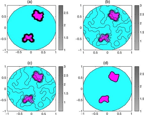
Let us present the results of the numerical experiments. The domain Ω is the unit circle. The triangular Delaunay mesh with N = 144 is constructed by the adaptmesh program of the MATLAB PDE toolbox [15]. Exact simulated data are chosen as the piecewise constant distribution of the basic permittivity value ε1 = 1 in the main part of the unit circle, and ε2 = 3 as the inhomogeneity. Graphs (a) in figures 2–4 demonstrate these distributions of ε and the triangular initial mesh. Approximated (noisy) values εi at the points of the mesh are obtained by disturbing the exact values with casual random errors, with error estimation δ = 0.5. These values simulate the output data that can be obtained by any method of reconstruction of the desired permittivity, particularly by the method realized in the EIT2D program suite of the EIDORS project [14]. Graphics (b) in figures 2–4 present the recalculation of these noisy data onto the regular mesh {xi, yi} with n = 21, 51, 101. Graphs (c) in all these figures explain the result of post-processing by the MATLAB filtering program medfilt2. Graphs (d) present post-processing by our proposed algorithm. Comparing graphs (c) and (d) in figures 2–4 we see the advantages of the algorithm developed.

Figure 2. Post-processing the model tomography image: n = 21,ϵ2 = 3.

Figure 3. Post-processing the model tomography image: n = 51,ϵ2 = 3.

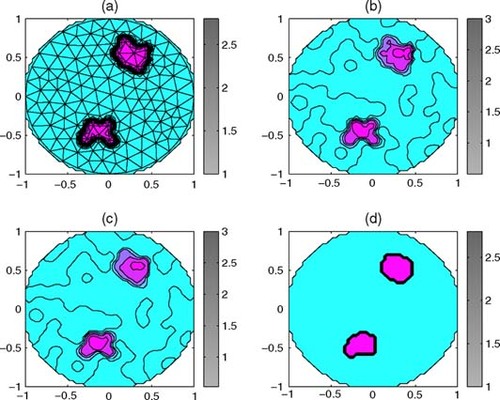
Figure 4. Post-processing the model tomography image: n = 101,ϵ2 = 3.

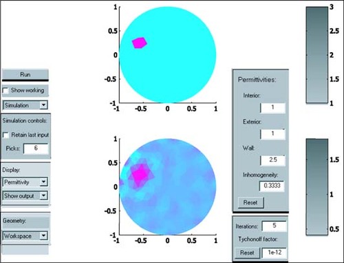
In figure 5 we have an example of the EIT2D application: the upper graph shows the distribution of the exact values ε, whereas the lower graph shows ε recuperated by EIT2D algorithms. To compare the results of EIT2D reconstruction with the post-processed ones using the proposed algorithm, we chose a finer mesh with n = 31, c = 1.2, and calculated for the considered example the estimation δ = 0.54 using images of the exact and reconstructed distribution of 1/ε .

Figure 5. Reconstruction of the permittivity distribution by the EIT2D program.

In figure 6 we present: (a) 1/ε recuperated by the EIT2D algorithms, (b) recuperation by formula (2)(2) and smoothing by (4)(4) –(7)(7) without projection on (--4) , (c) projection only to the set (--5) without smoothing, and finally (d) 1/ε recuperated by the developed algorithm (number of smoothing (--6) ).

Figure 6. Post-processing EIT2D image: n = 31ϵ2 = 3.

4. Image pre-reconstruction and data post-processing in ECT experiments

In figures 7–9 we present photographs of capacitance measurement experiments realized at the Instituto Mexicano del Petroleo (IMP) and the results after post-processing the LBP-reconstructed images using the proposed algorithm. Using an actual capacitance tomography system, various objects were placed inside the sensor and real capacitance measurements were taken. From those capacitance measurements, ‘pre-reconstructed’ images were generated using the LBP algorithm. The proposed post-processing methods were then applied on the images in order to improve them.

Figure 7. The experiment.

Figure 8. Pre-reconstructed by LBP image of the experiment.

Figure 9. Post-processed image of the experiment.

5. Conclusions

A fast algorithm for improving electrical capacitance tomography images is proposed for the case of two-phase flow regimes with known values of the permittivity of the mixture components. Its regularization properties are demonstrated in numerical experiments for simulated model examples.

Acknowledgements

The authors wish to thank the Instituto Mexicano del Petroleo for the support received for this research.