Aircraft parameter estimation using output-error methods

Abstract

Certification requirements, optimization and minimum project costs, design of flight control laws and the implementation of flight simulators are among the principal applications of inverse problem applications in the aeronautical industry. The problem of aircraft identification and parameter estimation demands for accurate mathematical model of the aerodynamics and adequate experimental flight data gathering and processing. The aircraft dynamic modeling is characterized by aerodynamic and control derivatives whose values can be directly determined from flight test data. This work describes the application of the output-error method using the Nelder–Mead (NM) and Levenberg–Marquardt (LM) algorithms to obtain the aerodynamic and control derivatives of a regional jet aircraft. Unlike others identification methods based on equation-error the output-error method gives unbiased parameter estimation in the presence of measurement noise. In this work, experimental results for estimation of the lateral directional aerodynamic derivatives, using flight test data provided by EMBRAER, are presented.

Keywords:

• Output-error
• Aircraft parameter estimation
• Modeling and simulation

1. Introduction

Modeling and simulation (MS) has become an integral part of the aeronautical industry design and evaluation processes. One of the major parts of MS is system identification and parameter estimation, applied to complex aerodynamic system such as an airplane. System identification is a general procedure to match the observed input–output response of a dynamic system by a proper choice of an input–output model and its physical parameters. Its application to aircraft systems involves many interdisciplinary aspects of aeronautical engineering 1 including: (i) design of maneuvers to optimize system identificability; (ii) development of flight data measuring techniques and digital data processing 2 for reduction of sensor noise and time delay for both input and output measurement processes; (iii) development of suitable flight mechanics models and corresponding flight simulation for synthetic data generation and mathematical prediction of maneuver response and (iv) development of parameter estimation methodologies to extract unknown physical aircraft parameters from flight test data. From this point of view, the aircraft system identification or inverse modeling comprises proper choice of aerodynamic models, the development of parameter estimation techniques by optimization of the mismatch error between predicted and real aircraft response and the development of proper tools for integration of the equations of motion within the system simulation and correlated activities 3.

This work focuses the determination of the stationary aerodynamic derivatives of a fixed wing regional jet airplane, using a linearized lateral directional model for the aircraft. The effectiveness of the implemented parameter estimation method was tested by matching real flight test data with the predicted response of the aircraft. Two algorithms were used to solve the associated optimization problem: (i) Nelder–Mead (NM) and (ii) Levenberg–Marquardt (LM) 4.

In the aeronautical industry, the output-error method is one of the most-used estimation methods for aerodynamic modeling and aircraft identification 4–6. This method has several desirable statistical properties and it is equally applicable to fully nonlinear dynamical systems, accounting for measurements noise 6.

In the first part of this work the airplane dynamic model and the problem of identification and parameter estimation are reviewed. Special attention was given to the Gauss–Newton and LM algorithm description. The maneuver chosen for identification and estimation purposes was a coordinated doublet for both the aileron and rudder inputs, denoted in the figure captions as δ a(t) and δ r(t), respectively. The results obtained by the two parameter estimation algorithms were compared using the same set of flight test data.

2. Model and estimation algorithm

The aircraft dynamic system is described by a stochastic nonlinear hybrid model in the form:

(1)

where x(t) is the continuous state vector, x0 the known initial state, u(t) is the control input vector and y(k) is observation vector measured on N discrete time. The vectors (a, c) and matrices (F, G) of the adopted model are functions of θ, the vector containing the parameters to be estimated. Depending on the aircraft model, the system functions (a, c) are nonlinear vector functions of the state and parameter vector. The matrices F and G are linear time-invariant matrices representing sensor and state perturbation effects. The process noise (ω), and measurement noise (ν), are assumed to be Gaussian white noise with zero mean and identity covariance matrix. The output-error method is well known to be sensitive to the process noise effects, which was not addressed in this particular work. In general, the assumption that the process noise is negligible must be thoroughly verified as was done in the present case where no turbulence effects were detected.

In this work the inverse problem formulation is applied to the lateral directional movement of the aircraft, for which the linear state and output equations can be written as 6,

(2)

The above dynamical equation has 14 unknown parameters that need to be estimated, giving θ∈R¹⁴,

(3)

As usually formulated in the aeronautical literature 5, 6, the components of the vector θ are the dimensional aerodynamic derivatives, e.g., , which in turn can be written in terms of nondimensional coefficients, e.g., CYβ, by proper choice of flight parameters, such as ρe,Ve, S,m, (all assumed) known a priori.

3. Estimation methods

The output-error method is one of the most-used estimation methods in aircraft identification and aerodynamic parameter estimation 1368. It has several desirable statistical properties, including its application to nonlinear dynamical systems and the proper accounting of measurement noise 4. The present inverse problem starts with the Gauss–Newton optimization process involving the output prediction error:

(4) (5)

where y(k + 1) is the measured output, is the prediction, and S is the sensitivity function, as defined in equation (8(8) ).

The cost function is written as 78,

(6)

The application of the standard Gauss–Newton procedure 57 for the minimization of the cost function results the following update for the unknown parameter, θ:

(7)

The cost function minimization needs the evaluation of the sensitivity function at the time (k+1). The sensitivity of the prediction error i, with respect of the unknown parameter j, is denoted by Sij(k + 1),

(8)

with ; k = 0,1, …, nr − 1, ; i = 1, …,no and j = 1, …,npar.

For a better understanding about the updated parameter , we investigate the Hessian of the cost. To do that, we rewrite equation (6(6) ) as: (9) where and .

The relationship between the sensitivity matrix S(k) and the Hessian is (10) and considering equations (6(6) ) and (9(9) ), it is noted that the recursion formula given in equation (6(6) ) needs the inversion of the Hessian matrix.

In this work the effectiveness of two output-error methods is compared, one is based on direct search simplex method 7 – the NM, and the other is based on a quasi-Newton methodology 57 – the LM. The advantage of the simplex method is that it does not need information about the cost function gradient as given by the error sensitivity function with relation to the estimated parameters. It only needs the direct cost function evaluation in terms of the prediction error. In this case, it is possible to apply both linear and nonlinear model parameterization.

For details on the Neder–Mead method, see for instance 9.

On the other hand, the quasi-Newton Levenberg–Marquardt method requires information about the gradient of the cost function and the Hessian 7. This method is a compromise between the cost function minimization and the need for keeping small parameter update. In this framework, the cost function is modified to

(11)

The minimization of the aforeseen relation results in the following modified parameter update equation,

(12)

where Δθ was calculated by solving the resulting system of algebraic equations by the singular value decomposition (SVD) method 8.

4. Matching of flight test data

The aerodynamic derivatives associated with the lateral directional model, as shown in equation (2(2) ), were estimated by matching the real flight test data with the model predicted simulation. A dutch-roll maneuver of a regional transport aircraft was used to investigate the effectiveness of the two discussed output-error methods: (i) the NM and (ii) the LM; applied to estimate the aerodynamic parameter vector defined in equation (3(3) ).

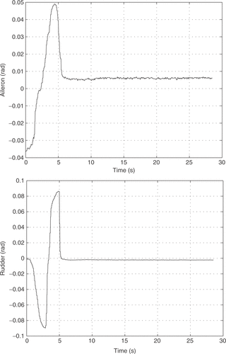
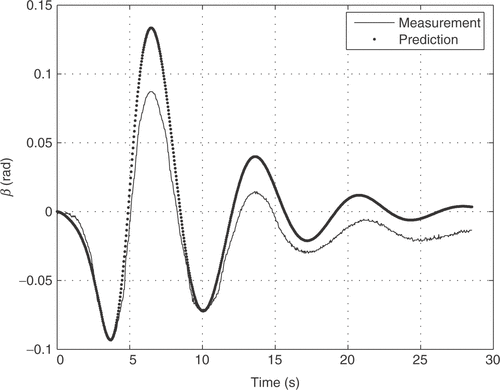
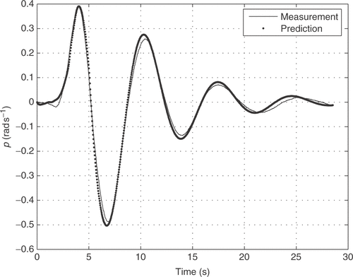
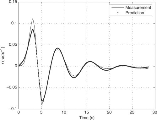
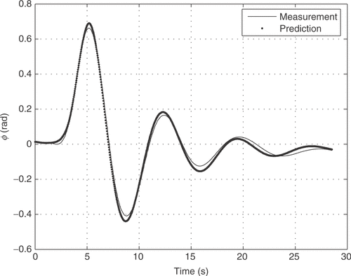
The aircraft input signals are the aileron δ a(t) and rudder deflections δ r(t) and the output signals are five attitude parameters: sideslip angle β(t), roll rate p(t), yaw rate r(t), bank angle φ(t) and lateral acceleration ay (t). The experimental input signals are shown in figure 1. The time history of the aircraft input–output relation was measured with a sampling time of 0.031 s, and the 914 measured points gives an observation time window of approximately 28 s.

Figure 1. Aileron (δ a) and rudder (δ r) inputs for the dutch-roll maneuver.

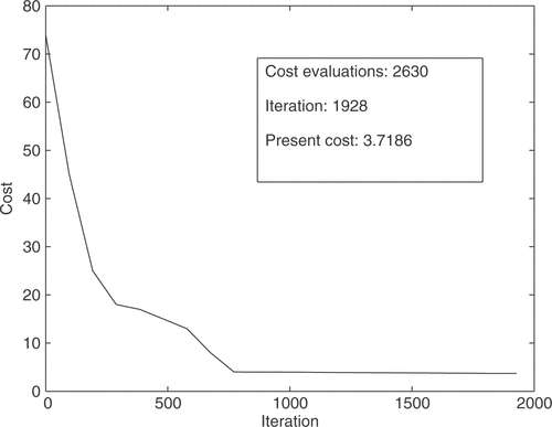
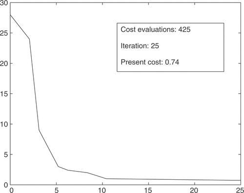
The efficiency of the two estimation methods can be assessed by comparing the evolution of the cost function. Figure 3 shows the cost function evolution of the NM method, while figure 3 shows the cost evolution for Levenberg–Marquardt algorithm. In the first case, around 1900 iterations are necessary to reduce the cost function to 3.72, while in the second case it takes only 25 iterations to significantly reduce values.

Figure 2. Cost function evolution with NM.

Figure 3. Cost function evolution with LM.

Table 2 shows the final values of the nondimensional aerodynamic derivatives obtained by the NM and the LM algorithms. The NM method was initialized with the values, displayed in the table. Then we use the values achieved with this method to initialize the Levenberg–Marquardt algorithm, since this method is more computationally demanding and so a good estimate can speed up convergence. In the results reported below, a quadratic cost with weighting factor equal to one is used. A maximum likelihood cost could also be used, in which case the weighting factor would be the estimated covariance matrix associated to the prediction errors.

Since the flight data employed to generate table 1 was obtained experimentally and no wind tunnel tests are available, there are no true parameter values for deciding which method achieved the best performance. For this, an indirect measure of performance is used based on the prediction error. So, the main focus of the present inverse aerodynamic modeling is to check that this local minimization procedure can result on good matching to the experimental flight data and stable input–output relation for the aircraft. This prediction capability, as obtained by the two output-error methods, can be accessed from the model validation results.

Table 1. Estimation of the nondimensional stability and control derivatives.

Coefficient	Initial values	NM method	LM method
CYβ	−0.0068	−0.0077	−0.0058
CLβ	−0.1861	−0.1821	−0.1514
CLP	−0.3562	−0.3272	−0.4718
CLr	−1.1700	1.6393	1.4942
CNβ	0.0678	0.0644	0.0415
CNP	0.0616	0.0538	−0.0275
CNr	−2.7110	−1.2157	−0.6765
	0.0068	0.0099	0.0052
	−0.0068	−0.0079	−0.0073
	−0.0001	−0.0032	−0.0029
	−0.0198	0.0623	0.0704
	0.0016	0.0023	−0.0405
	−0.2037	−0.1147	−0.1029

Table 2. RMS error for the outputs.

Variable	Nelder–Mead	Leverberg–Marquardt
β	0.0143	0.0131
p	0.0142	0.0132
r	0.0054	0.0045
φ	0.0205	0.0143
ay	0.0187	0.0143

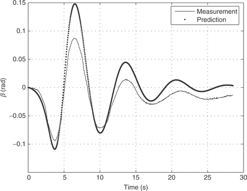
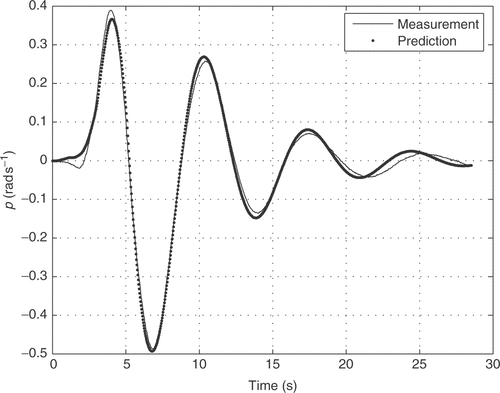
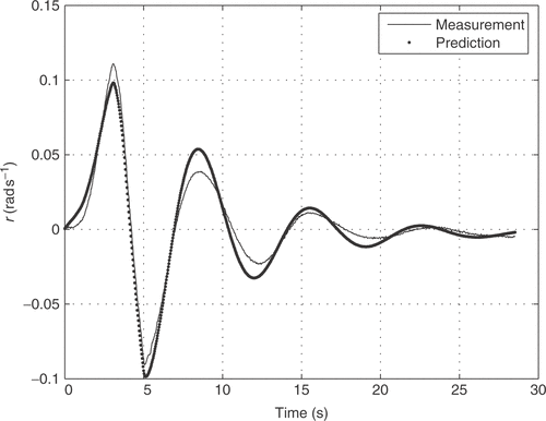
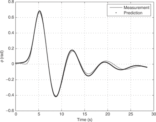
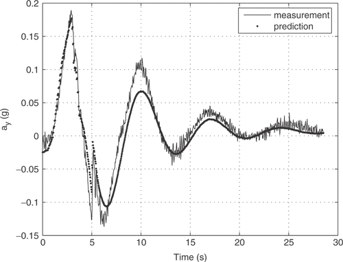
Figures 4–8 show that, the flight data matching achieved with the NM method provides a good initial parameter estimation procedure, since the final prediction error is reasonable. In the LM algorithm (figures 9–13), the estimation error was smaller, compared to the NM algorithm, but higher computational processing time was demanded.

Figure 4. Measured sideslip angle β(t) and estimated values by the NM method.

Figure 5. Measured roll angular velocity p(t) and estimated values by the NM method.

Figure 6. Measured yaw angular velocity r(t) and estimated values by the NM method.

Figure 7. Measured roll angle φ(t) and estimated values by the NM method.

Figure 8. Measured lateral acceleration ay (t) and estimated values by the NM method.

Figure 9. Measured sideslip angle β(t) and estimated values by the LM method.

Figure 10. Measured roll angular velocity p(t) and estimated values by the LM method.

Figure 11. Measured yaw angular velocity r(t) and estimated values by the LM method.

Figure 12. Measured roll angle φ(t) and estimated values by the LM method.

Figure 13. Measured lateral acceleration ay (t) and estimated values by the LM method.

In a similar way, the same quantitative results were obtained with the application of the Levenberg–Marquardt match the flight data as shown in figures 10–13.

Although the figures lead visually to the conclusion that the Levenberg–Marquardt method performed better, this conclusion can be formally reached by looking at the accumulated prediction error (cost function) 3.72 for the Nelder–Mead method, and 0.74 for Levenber–Marquardt.

Besides, we calculated the root mean square (RMS) error for the various outputs, to quantify the difference between model output and measurement, for the two approaches and show the results in table 2. We observe that, for all the outputs the Levenberg–Marquardt method presented lower RMS error.

5. Conclusions

The results obtained in this work compared two output-error methods: the Nelder–Mead (NM) and Levenberg–Marquardt (LM) algorithm to inverse modeling of an aircraft. The estimation of linear aerodynamic derivatives was computed by minimization of a cost function based on the predicted output error. Both the direct simplex (NM) and the quasi-Newton methods (LM) presented good convergence properties and resulted in good match to the experimental flight data. The parameter identification by both methods gave consistent results, except for the values of four aerodynamic derivatives (see table 1), showing that different local minimum can provide good predictive capabilities. The NM method can be used as an initial estimation procedure for the more refined search algorithm based on the local gradient function. Some other refinements could be achieved by weighting the cost function with the inverse of the estimated sensor noise covariance 57. In conclusion the Levenberg–Marquardt algorithm has a better performance but the computational associated with the calculation of the sensitivity functions are much higher. Additionally, the Nelder–Mead method can be useful for larger order problems.

Acknowledgments

This work was sponsored by FAPESP (Fundação de Amparo Pesquisa do Estado de São Paulo), through the partnership project EMBRAER/ITA, as part of the PITE Program.

References

- Hamel, PG, and Jategaonkar, RV, 1996. Evolution of flight vehicle system identification – survey paper, Journal of Aircraft 33 (1996), pp. 9–28.
- Hemerly, EM, 2000. Controle por Computador de Sistemas Dinâmicos. Sao Paulo, SP: Edgard Blucher; 2000.
- Jategaonkar, RV, and Thielecke, F, 2002. ESTIMA– an integrated software tool for nonlinear parameter estimation, Journal of Aerospace Science and Technology 6 (2002), pp. 565–578.
- Maine, RE, and Iliff, KW, 1975. "A Fortran program for determining stability and control derivatives from flight data". In: Technical report D-7831, NASA.; 1975.
- Maine, RE, and Iliff, KW, Identification of dynamic systems – theory and formulation. Reference publication 1138, NASA. 1975.
- Maine, RE, and Iliff, KW, Application of parameter estimation to aircraft stability and control – the output-error approach. Reference publication 1168, NASA. 1975.
- Nelles, O, Nonlinear System Identification. Kronberg: Springer.
- Neto, WR, Hemerly, EM, and Ges, LCS, 2003. Aircraft identification using output-error methods. Paper presented at the 2nd Conference on Dynamic and Control Applications. Brazil, .
- Press, WW, Flannery, BP, and Teukolsky, SA, 1990. Numerical Recipes in C. The Art of Scientific Computing. New York: Cambridge University Press; 1990.