Abstract
The accurate simulation of lead-acid batteries requires the use of sophisticated models based on first principles containing many parameters. Existing methods for parameter identification often fail due to many local minima of the error function or the high computational needs to cover the parameter space. Therefore, a novel approach for parameter identification with complex physical models containing many unknown parameters is presented. It is based on the utilization of available expert knowledge regarding specific model parameters. The expert knowledge is integrated through fuzzy control and combined with stochastic optimization algorithms for solving the battery identification problem.
1. Introduction
The accurate simulation of lead-acid battery cells is of growing interest in the automotive industry, especially in hybrid and electric vehicle technology. The battery is a fundamental component of the powertrain of such vehicles. Its nonlinear behavior under various operating conditions has to be considered for the implementation of new drive concepts. Various models for lead-acid batteries exist which are based on a detailed description of the electrochemical, thermal, and transport processes in the battery Citation1–5. The models consist of systems of partial differential equations that are highly nonlinear and depend on several different parameters. Many of them can only be measured with elaborate, often destructive methods, while some cannot be measured at all. The only quantities that are easily accessible are the cell voltage and the cell current. There is an increasing need for a fast parameterization of the battery models at low cost since the parameters of batteries from different manufacturers show considerable differences. In addition, the values depend on the state of health of the battery. They are slowly changing with time. This long-time behavior of the batteries cannot be predicted by present models. A frequent re-parameterization is therefore necessary.
Classical approaches to parameter identification very often fail to satisfy the demands for accuracy and speed. A new approach for parameter identification of batteries was therefore developed. It tries to utilize all available knowledge about the model parameters to achieve a better performance. The method is solely based on the measurements of cell current and cell voltage. These quantities can be obtained very easily and with low cost. The available expert knowledge is built into a fuzzy controller Citation6. The resulting control loop is embedded in a genetic algorithm (GA) Citation7.
The following section gives an introduction to the used lead-acid battery model. After that, the novel parameter identification method is described in detail, including the accumulation of expert knowledge, the fuzzy control loop, and the GA. The identification results for a real battery are presented next, followed by some concluding remarks on the presented identification method and future developments.
2. Lead-acid battery model
The used battery model (based on Citation1–5) describes a single lead-acid battery cell with starved electrolyte. Originated on electrical, chemical, thermal, physical and material transport phenomena the formulation is based on a macroscopic description of porous electrodes. The cell consists of a porous PbO2 electrode with conductivity σ1, a porous Pb electrode with conductivity σ3, and a porous non-conducting separator in between ().
Figure 1. Cross-section of the cell model: porous PbO2 (left, region 1) and Pb (right, region 3) electrodes; a porous separator (middle, region 2).
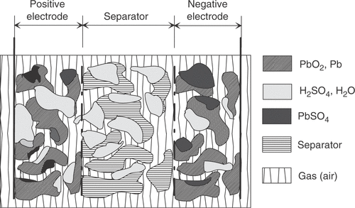
Acid with conductivity κ is present in each of the regions. For the model it is a reasonable simplification to consider space coordinates in only one dimension (thus all quantities are related to the geometrical area of the electrodes).
The amounts of the materials, which are functions of space and time are described by volume fractions for the solid and for the liquid phase (ϵs and ϵl):
(1)
(2)
jmain, jO2, and jH2 are the current densities due to the main charge/discharge-, oxygen-, and hydrogen-reaction which are defined separately for regions 1 and 3 labelled by an additional subscript, as:
(3)
(4)
(5)
(6)
(7)
(8)
Due to the double layer capacity Cdl at the interface between the solid and the liquid phase an additional term has to be defined:
(9)
The total current density can thereby be calculated as
(10)
The overpotentials η, ηO2 and ηH2 are defined as
(11)
and the terminal voltage can be calculated by
(12)
Two further equations have to be considered expressing Ohm's law in the liquid phase
(13)
and Ohm's law in the solid phase
(14)
The acid concentration cA is calculated separately near the interface of the solid and liquid phase for a small constant volume ϵl, near and further away:
(15)
(16)
The local utilization of the active material
is defined by
(17)
The constants Kx only depend on the geometry of the cell whereas the coefficients Lx also depend on temperature, acid concentration, and cell pressure. The values of the coefficients, as well as the capacity density of the electrode active material Qmax are known from the relevant literature cited in this section. The functions fx(·) show a nonlinear dependance on their arguments. The values of the remaining coefficients are treated with the parameter identification algorithm described next. For a more detailed description of the model the reader is referred to Citation1–5.
To solve this set of differential equations the control volume method as described in Citation3, Citation5, Citation8 is applied.
3. Parameter identification
The parameter identification algorithm is used to estimate the initial values of all relevant unknown parameters. The lead-acid battery model contains 24 unknown parameters in total. The acid concentrations cA, near and cA, far, the solid volume fraction ϵs, the liquid volume fraction ϵl and the utilization of the active material
are spatially distributed. Their initial values are however assumed constant within the regions of the cell. This is a valid simplification if the battery is carefully discharged with a low current to equalize the material distributions. Some parameter values can be deduced from other parameters. The utilization in region 1 is set to 1.6 times the utilization in region 3 according to the usual composition of the active electrode materials in lead-acid cells, and the double layer capacity in region 3 is 10% of the value in region 1. The initial volume fraction of the solid phase ϵs is inversely proportional to the initial liquid phase fraction ϵl. A long rest period prior to the reference measurement ensures a constant acid concentration in the whole cell, allowing us to estimate a joint value for the acid concentrations c A, near near the interface and cA, far in the bulk region. When the battery is discharged, αa in region 1 of the cell and αc in region 3 can be neglected compared with their influence in the other regions. The opposite holds when the battery is charged. Therefore, αa in region 1 and αc in region 3 are assigned the same value, and αa in region 3 and αc in region 1 also share a common value.
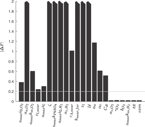
The aforementioned assumptions lead to a number of 22 unknown parameters. The result of a sensitivity analysis for the unknown model parameters is depicted in . The bar plot shows the change in the error function (19) used for the parameter identification for a 1% deviation of the respective model parameters. A manually fitted parameter vector yielding reasonable simulation results was used as nominal point. It can be seen that the influence of α c, O2, γO2, δO2, amaxk m H2, ex and exm (ex and exm appear in the functions fx of the model equations) can be neglected. The remaining 16 parameters with a sensitivity above 0.2 are estimated with our parameter identification approach.
Figure 2. Sensitivity coefficients of the model parameters (change in the error function F (19) with respect to 1% variations of the model parameters starting from a manually fitted model). The highest sensitivity values are truncated at Δ F=2.
The cell voltage shows a highly nonlinear dependance on the model parameters. The error function, e.g. the sum of squared errors, contains many local minima that result in unacceptable identification results. Therefore deterministic local optimization algorithms, like the Gauss–Newton algorithm, are not well suited for the parameter identification Citation9. Global stochastic optimization methods, like GAs, have shown to be capable of finding the global optimum of multimodal functions. However, the necessary population size for a good coverage of the parameter space results in a very high computational burden in combination with the complex and time-consuming simulation model.
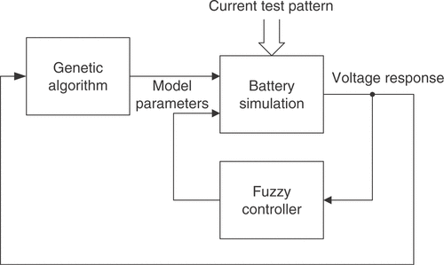
With the proposed identification algorithm, it is tried to reduce the number of simulations needed to obtain satisfactory results. Available expert knowledge about the lead-acid battery model is utilized during the identification process. The expert knowledge can be obtained from an analysis of the model equations and from experiments with the cell model. It is a qualitative description of the influence of several battery parameters on the voltage response of the model. Some parameters, e.g., may only affect a certain characteristic of the model response in a monotonic way. In this context, the extraction of characteristic quality criteria from the model response, as further described in section 3.2, is of particular importance. The information can be used to estimate the optimal values of these parameters by means of an expert system. A fuzzy inference system embedded in an optimization loop is used for this purpose Citation10. However, the influence of a number of parameters on the simulation results cannot be predicted precisely. Some model characteristics may also be influenced by more than one parameter, leading to ambiguity. These parameters are consequently treated with a GA. The resulting combination of fuzzy control and a stochastic optimization algorithm considerably reduces the computational demands of the stochastic algorithm due to the smaller dimension of the search space while maintaining its global search capabilities.
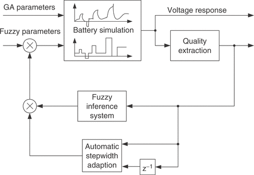
The structure of the combined identification method is shown in . Based on the current population, the GA manipulates the individuals to generate a new population according to the principles of evolution Citation11. This results in new combinations of the parameters with unpredictable behavior. The remaining parameters are adjusted with a control loop containing the fuzzy expert system. The difference between the simulated and measured voltage responses of the battery is resolved into several different quality criteria. They are calculated under consideration of the specific current test pattern used as excitation signal. Every criterion rates a certain aspect of the quality of the simulated parameter vector. The performance numbers are closely linked to the expert knowledge. The fuzzy inference system changes the battery parameters according to the calculated qualities and its rule base. This inner optimization loop is repeated until some stopping criterion is reached. It can be regarded as a control loop that tries to compensate the difference between measurement and simulation by adjusting the fuzzy controlled parameters. After the inner loop is terminated, the next iteration of the GA is launched.
Figure 3. Block diagram of the parameter identification algorithm.
3.1. Excitation signal
A special current pattern was designed for the identification process, and is depicted in . The curve was carefully chosen to excite all internal states of the battery. It contains charge and discharge pulses of different durations to cover transient effects. Additionally, the static changes of the battery behavior with the state of charge are recorded by repeated application of the pulse pattern during a constant current charging of the battery. The nonlinear relationship between cell voltage and current intensity is covered with different pulse amplitudes. The excitation signal can be used for lead-acid cells of different capacities by scaling the applied currents according to the cell capacity.
Figure 4. Current pattern used for battery identification.
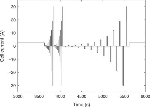
The measurement starts with a completely discharged battery. First, the 20 h charge current is applied for 1 hour in order to reach a certain state of charge of the cell. After that the pulse pattern of is applied. The first part consists of a set of 20 alternating charge and discharge pulses of short duration. The pulse time should be short enough so that the effect on the acid concentration in the cell is negligible (for the used cell this led to a pulse duration of 0.13 s), such that the voltage response is mainly a function of the double layer capacity. The current intensity is increased with a constant ratio between adjacent pulses. The same pulse block is then applied one more time to verify that no major change in acid concentration occurred during the first application of the pulse pattern. After that comes another set of 20 alternating charge and discharge pulses, but with a longer duration and a longer idle time between them. These times are chosen dependent on the desired field of application. For the usage in a hybrid vehicle a pulse duration of 15 s (typical pulse power charge respectively discharge durations in the New European Driving Cycle) and an idle time of 60 s were applied. After applying the pulse pattern the battery is further charged with the 20 h charge current for 1 h before the whole current pattern of is applied again. This process is repeated until the pressure in the battery reaches a predefined limit. Excessive gassing reactions begin after the cell is fully charged and cause the pressure rise, marking the limit of the usual operating range of the battery. The measurement of the whole voltage response of a real cell may take up to 25 h.
The battery should be completely discharged before applying the test pattern. The discharge should be performed with a small current (e.g. 10–20 hour discharge) in order to equalize the material distributions within the cell. A rest period should follow after that to obtain a constant acid distribution. These steps are necessary to justify the simplifications made regarding the spatial uniformity of the initial values of some battery parameters.
3.2. Error function and quality criteria
The most common choice for the error function F of identification problems is the sum of squared prediction errors Citation12. It offers favorable properties when used with least squares optimization algorithms, but since we use a GA arbitrary error functions are equally applicable. The sum of squared errors equals the maximum likelihood method for Gaussian corrupting noise. However, the measurement noise of our setup is negligible. The sum of absolute errors is better suited for our purpose due to the properties of the battery model and the excitation signal. The excitation consists of long periods with a small constant charge current and short high-current pulses. The model output is equidistantly sampled to obtain n discrete values to make up the objective function. The largest errors usually occur during the high charge and discharge pulses. The sum of squared errors tends to penalize large errors while it is insensitive to small errors. This is not desirable for our approach since a good simulation accuracy during the long constant current charge periods is a major concern. Therefore, we use the sum of absolute errors which equally weights all errors,
(18)
with the voltage response of the model UM and the measured cell voltage U. The disadvantage of (18) is that the model responses to different excitations, like charge pulses, idle times, and discharge pulses are merged into one number. Some model parameters influence all the characteristic model responses. But there are also parameters that only act on specific characteristics. This information is lost by summing up the errors.
The fuzzy expert system needs more specific information to incorporate available expert knowledge to adjust some of the battery parameters. Therefore, the voltage response of the cell is broken down into several distinct battery characteristics. These quality criteria may be mainly influenced by certain parameters only, allowing the isolated adjustment of these parameters in order to fit the model to a real battery. For that purpose 11 quality criteria Qi are extracted from the simulated and measured voltage responses. Each of them is a measure of the difference between a certain detail of the real cell behavior and the model response. The criterion Q1 is the voltage deviation at the low charge current between the pulse sequences, averaged over the whole state of charge, as illustrated in . The difference in the slopes of the low charge current responses shown in the figure is rated by Q2. Q3 describes the difference of the open circuit voltages during the idle time between the short and long pulse sequences, as depicted in . The value is averaged over all pulse sequences. The performance measure Q4 is the difference of the heights of the voltage responses to a charge current pulse, as illustrated in , while Q5 reflects the same characteristic for the discharge current pulses. The value is averaged over all pulse sequences between the start of the measurements and the start of excessive gassing reactions. The average height of the short charge and discharge pulses is assessed through Q6, as shown in . The increase in the voltage peaks between the subsequent long current pulse sequences is rated with criterion Q7. With Q8 the slope of the open circuit voltages from is addressed. The described criteria are only calculated from the voltage response before excessive gassing reactions start in the cell. This is characterized by a sharp rise in the cell voltage and cell pressure even at low charge currents, because the utilization of the active cell materials approaches zero. The time of this rise is rated by quality criterion Q9, as shown in . Finally, the criteria Q10 and Q11 are the counterparts of Q4 and Q1 after the voltage rise due to gassing.
Figure 5. Quality criterion Q1: difference of the voltages at low charge current.
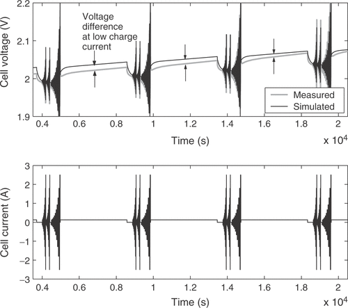
Figure 6. Quality criterion Q3: difference of the open circuit voltages.
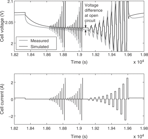
Figure 7. Quality criterion Q4: difference of the height of the voltage response to a charge current pulse.
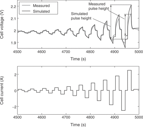
Figure 8. Quality criterion Q6: difference of the peak–peak amplitudes of the short pulse responses.
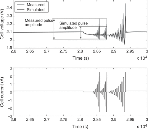
Figure 9. Quality criterion Q9: difference of the time of voltage rise when the battery is fully charged.
The sum of absolute values of the quality characteristics is also a measure of the total model quality. However, only certain major effects that are of special interest to the user can be sampled. Small deviations between real cell and model cannot be tracked with the quality measures. By using the sum of the qualities as error function, the emphasis can be put on identifying the most important battery characteristics. For the present approach a combination of the sum of absolute values of the prediction errors and the sum of quality measures is used:
(19)
The weight w1 determines the compromise between sampling the major effects only and evaluating the overall performance of the model. It is chosen to balance the contributions of the single terms
3.3. Genetic algorithm
A floating point GA Citation7, Citation11 is used as stochastic optimization strategy for the battery parameters that cannot be handled with the fuzzy expert system. In our case that concerns the seven parameters ζ, ϵ l,near, amaxkPbSO4, amaxi0, αa, O2, amaxi0, O2 and amaxkm,O2. Some of them have an unpredictable influence on the model, which cannot be simply represented by a monotonic relationship. The others may have a predictable influence on one of the quality criteria, but there is another parameter that features a higher sensitivity. Then the parameter with the highest sensitivity is tuned with the expert system, while the other is left over for the GA in order to avoid ambiguity.
For every individual, the GA calls the inner fuzzy optimization loop. The inner loop performs some iterations and returns the error function value of the individual. The fitness of the individuals is determined based on a linear ranking of the error function values (equation 19) of the population. The selection of a part of the population for recombination is made with stochastic universal sampling Citation11. The recombination probability of the individuals is proportional to their fitness. The following recombination operation generates new individuals from the selected parents by intermediate crossover Citation7. The parameters of the new individuals are mutated with a low probability. The mutation range follows a normal distribution. The fitness of the new individuals is calculated after invoking the inner optimization loop. They are afterwards reinserted into the population. The GA is based on an elitist strategy. The individuals with the lowest fitness are always discarded in favor of the new ones. The next iteration is started with the selection until a stopping criterion causes the termination of the algorithm. In our case, the algorithm is terminated if there is no improvement of the error function of at least 2% in three generations.
3.4. Fuzzy expert system
The nine battery parameters a maxi0, H2 αc,H2, cA, knear, far, ϵl,
, αa, αc and Cdl are estimated with the fuzzy expert system. It adjusts the parameter values for a given set of GA optimization parameters to give the best possible model response Citation10. The block diagram of this inner optimization loop is shown in . The battery parameters given by the GA are fed into the model and remain constant during the following steps. The initial values for the inner optimization parameters are taken from the individual of the preceding GA generation that is closest to the current individual. This is a kind of information sharing between the individuals of different generations. The battery simulation is performed with the initial parameter values in the first iteration. Afterwards, the quality criterions are calculated from the voltage response. They are used as inputs of the fuzzy controller, which is implemented as a linguistic (Mamdani-type) fuzzy inference system Citation13. Based on the expert knowledge formulated in rules, the controller produces output factors. The battery parameters are multiplicatively connected with the factors. The subsequent iteration is started with the modified fuzzy loop parameters. The inner loop is terminated if the prescribed maximum number of iterations is reached or if there is no significant improvement. The automatic stepwidth adaption is monitoring the actual and preceding values of the quality measures. If the fuzzy output factors are shown to be too conservative or too big, the stepwidths of the fuzzy outputs are multiplicatively altered.
Figure 10. Block diagram of the internal fuzzy control loop.
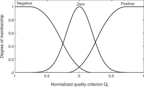
The input variables of the fuzzy system are normalized and then fuzzified with the three membership functions negative, zero, and positive as shown in . Gaussian and spline-based function definitions are used. Similarly, the fuzzy outputs consist of three membership functions: smaller, equal, and bigger. The minimum and maximum operators are used for the and-operation, implication, and accumulation. Defuzzification is performed with the center of gravity method Citation13.
Figure 11. Membership functions for the linguistic variables Qi.
The expert knowledge was accumulated by analyzing the underlying system of partial differential equations, the sensitivity coefficients of the parameters and by performing simulation studies. It is a qualitative description of the influence of some battery parameters on the quality characteristics Qi of the model output.
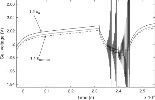
A number of 33 rules was established for the fuzzy controller. They combine at most two input variables with two output factors. The parameters cA and knear,far, e.g., mainly impact the quality criteria Q1 and Q3. Their influence on the model output is illustrated in . An increase in the initial acid concentration cA causes a constant displacement of the curve towards higher potentials, thus increasing both Q1 and Q3. An increase of knear,far results in a lower voltage during the 20 h charge current, while the open circuit voltage remains virtually unchanged, thus causing a decline of Q1 only. So both Q1 and Q3 can be minimized by suitably adjusting the two parameters. The correlations are formulated as nine rules covering all combinations of the linguistic values of the quality criteria. Some of the rules are:
Figure 12. Influence of cA and knear, far on the model response. The grey curve shows the nominal response, the massive black curve shows the response with cA increased by 20%, and the dashed black curve was obtained with knear, far increased by 10%.
IF Q1 = positive AND Q3 = positive THEN knear, far = equal AND cA, near = smaller
IF Q1 = positive AND Q3 = negative THEN knear, far = bigger AND cA, near = bigger
IF Q1 = positive AND Q3 = zero THEN knear, far = bigger AND cA, near = equal
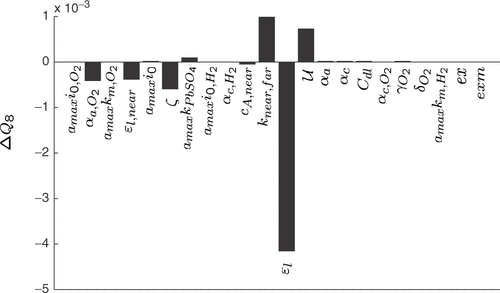
The sensitivity of the open circuit voltage, corresponding to Q8, with respect to the cell parameters is depicted in . The criterion is predominantly influenced by ϵl. Therefore, simple rules for ϵl can be set up:
Figure 13. Sensitivity coefficients of the quality criterion Q8 (slope of the open circuit voltage) with respect to 1% variations of the model parameters, starting from a manually fitted model.
IF Q8 = positive THEN ϵl = bigger
IF Q8 = negative THEN ϵl = smaller
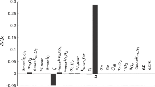
A similar situation arises for Q9 rating the start of excessive gassing. As can be seen from , it is mainly dependent on the utilization of the active material
. The corresponding rules are:
Figure 14. Sensitivity coefficients of the quality criterion Q9 (voltage rise due to gassing) with respect to 1% variations of the model parameters, starting from a manually fitted model.
IF Q9 = positive THEN
= smaller
IF Q9 = negative THEN
= bigger
The sensitivity coefficients regarding the amplitudes of the short charge and discharge pulses, Q6, are shown in . The short pulses were especially chosen to show the influence of the double layer capacity Cdl. However, Q6 is most sensitive to ζ and
due to the striking effect of these parameters on the model for high states of charge. Nevertheless, Cdl is used to adjust Q6 because the utilization is already used to control the time of the sharp voltage rise, where its sensitivity is much higher than for Q6. The exponent ζ has a very strong influence on most parts of the model response. Therefore, it cannot be used in the fuzzy control loop but is optimized by the GA. The utilization is implicitly included in the rules through Q9 due to its strong influence on the pulse heights, e.g.:
Figure 15. Sensitivity coefficients of the quality criterion Q6 (amplitudes of the short charge and discharge pulses) with respect to 1% variations of the model parameters, starting from a manually fitted model.
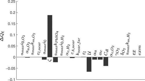
IF Q6 = zero AND Q9 = positive THEN Cdl = bigger
IF Q6 = positive AND Q9 = positive THEN Cdl = bigger
IF Q6 = positive AND Q9 = negative THEN Cdl = equal
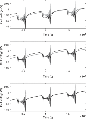
The argumentation for the remaining fuzzy-controlled parameters closely follows the aforementioned remarks. A demonstration of the performance of the fuzzy optimization loop is given in . The upper subplot compares the simulated voltage response after the first simulation run with the measured cell voltage. There is a distinct deviation of the simulation. The situation after the third iteration shows clear improvement, as depicted in the central subplot. After five calls of the simulation, the fuzzy control loop achieved a very good fit of the model.
Figure 16. Performance of the internal fuzzy control loop: simulated (black) and measured (gray) voltage responses after the first, third and fifth iteration.
4. Identification results
The proposed identification algorithm was tested on several real lead-acid batteries. As an example, the identification results for a battery of the type Hawker Cyclon with a nominal capacity of 5 Ah are shown. The reference measurements were taken at an ambient temperature of 20° C. The proposed excitation signal was applied with a maximum charge and discharge current of 5 A.
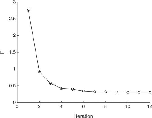
The identification algorithm was tested with different population sizes of the GA. It was found that the number of iterations before the algorithm terminates is almost independent of the population size. This may stem from the scarce coverage of the parameter space and the influence of the fuzzy control loop that also affects the fitness values of the GA population, leading to a premature termination at local minima. A population of 50 individuals already leads to reliable and reproducible reconstruction results. The presented solution was obtained with 50 individuals and converged after 12 GA iterations. The error function values of the best individuals of the respective generations are depicted in .
Figure 17. Evolution of the error function over the GA iterations.
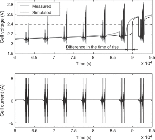
The estimated cell parameters are summarized in . The complete reference curve of cell voltage and the identification result are depicted in . The response to a pulse sequence at a low state of charge of the cell is shown in detail in . The response at a high state of charge, where excessive gassing occurs, is illustrated in . It can be seen that there is a very good agreement between model and real cell regarding the overall cell behavior. The integral of the cell voltage of for the real cell amounts to 52.50 Vh. The simulation gives a value of 52.53 Vh, which is a relative error of only 0.05%.
Figure 18. Identification result for a Hawker Cyclon 5 Ah lead-acid cell.
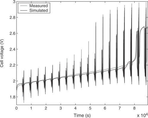
Figure 19. Detail of the identification result: pulse sequence at low state of charge.
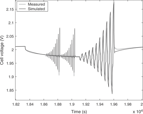
Figure 20. Detail of the identification result: pulse sequence at high state of charge.
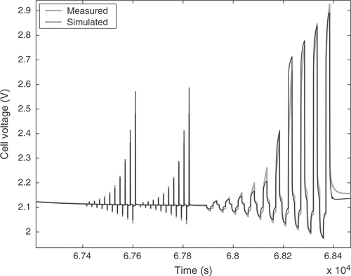
Table 1Estimated cell parameters for a Hawker Cyclon 5 Ah cell at 20°C.
However, the short-time transient behavior shows clear deviations. This is solely due to the imperfections of the model. For the desired applications the model has to deal with time constants from several milliseconds to hours, which requires some compromise between tractability and short-time accuracy. In addition, some of the dynamic processes in the cell are not fully understood yet. The model error nearly solely consists of a bias term resulting from the mentioned limitations. The measurement noise of our setup has a standard deviation of 47 µV for the raw voltage measurement, giving a minimum signal-to-noise ratio of 93 dB. The standard deviation of the raw current measurement is 720 µA. The influence of the measurement noise is further reduced due to the large raw data set consisting of 670 000 samples, so that the parameter variance can be safely neglected.
Altogether, the combination of the physical battery model and the proposed identification algorithm leads to a reasonable prediction of the cell behavior in the whole range of the state of charge and the arising time constants.
5. Conclusion
An accurate lead-acid battery model consisting of a system of nonlinear partial differential equations was presented. It depends on a variety of parameters that strongly vary for different batteries and even change during battery life. The parameters are hardly accessible for measurement or cannot be measured at all. Periods of up to 25 h may have to be simulated for parameter identification, which makes the solution of the forward problem very time-consuming. Common methods for parameter estimation often fail due to the computational demands and the severe nonlinearity of the model. Therefore a novel approach for the identification of the battery parameters was developed that integrates readily available expert knowledge regarding the influence of parameters on specific battery characteristics. These parameters are adjusted by a fuzzy controller containing the expert knowledge. The fuzzy control loop is invoked by a GA that optimizes the unpredictable parameters. The presented results suggest that the incorporation of available expert knowledge allows for a faster and more robust estimation procedure. The parameterization of a real cell shows that the novel method is able to provide good and robust results that can be used in a wide range of operating conditions. Due to the specialized expert knowledge, the method is only applicable to battery identification problems. Future research will be focussed on extending the method to a more general class of problems by automatic accumulation of expert knowledge from training data sets.
References
- Bernardi, DM, and Carpenter, MK, 1995. A mathematical model of the oxygen-recombination lead-acid cell., Journal of the Electrochemical Society 142 (1995), pp. 8–2631.
- Newman, J, and Tiedemann, W, 1997. Simulation of recombinant lead-acid batteries., Journal of the Electrochemical Society 144 (1997), pp. 9–3081.
- Gu, WB, Wang, CY, and Liaw, BY, 1997. Numerical modeling of coupled electrochemical and transport processes in lead-acid batteries., Journal of the Electrochemical Society 144 (1997), pp. 8–2053.
- Schweighofer, B, Steiner, G, and Brandstätter, B, Simulation of the dynamic behavior of a lead-acid cell. Presented at Proceedings of the IASTED International Conference on Modelling and Simulation 2003. 2003.
- Schweighofer, B, and Brandstätter, B, 2003. An accurate model for a lead-acid cell suitable for real-time environments applying control volume method., The International Journal for Computation and Mathematics in Electrical and Electronic Engineering 22 (2003), pp. 3–703.
- Hsu, Y-L, Lin, Y-F, and Sun, T-L, Engineering design optimization as a fuzzy control process. Presented at Proceedings of the 4th IEEE International Conference on Fuzzy Systems. 1995.
- Michalewicz, Z, 1996. Genetic Algorithms + Data Structures = Evolution Programs. Berlin: Springer-Verlag; 1996.
- Patankar, SV, 1980. Numerical Heat Transfer and Fluid Flow. New York: Hemisphere Publishing Corporation; 1980.
- Assis, EG, and Steffen, V, 2003. Inverse problem techniques for the identification of rotor-bearing systems., Inverse Problems in Engineering 11 (2003), pp. 1–39.
- Oltean, G, Miron, C, Zahan, S, and Gordan, M, A fuzzy optimization method for CMOS operational amplifier design. Presented at Proceedings of the 5th IEEE Seminar on Neural Network Applications in Electrical Engineering. 2000.
- Man, KF, Tang, KS, and Kwong, S, 1996. Genetic algorithms: concepts and applications., IEEE Transactions on Industrial Electronics 43 (1996), pp. 5–519.
- Nelles, O, 2001. Nonlinear System Identification. Berlin: Springer; 2001.
- Sugeno, M, 1995. Industrial Applications of Fuzzy Control. New York: Elsevier Science Pub. Co.; 1995.