Numerical methods for the reconstruction of dynamic magnetic resonance images

Abstract

The aim of this article is to present some numerical methods for the reconstruction of dynamic magnetic resonance images using a priori information. The methods are presented through a unifying algorithmic framework based on a generalized series representation of the dynamic image. We propose, in particular, the use of B-spline basis functions for the image representation and the use of regularization methods for the solution of the systems arising in the reconstruction process. Numerical experiments on both simulated and real data show that the proposed methods improve the quality of the reconstructed dynamic images over the traditional methods.

Keywords:

• Dynamic magnetic resonance imaging
• Regularization
• B-spline
• AMS Subject Classifications:
• 65D07
• 65F22
• 47A52
• 65R32

1. Introduction

Magnetic Resonance Imaging (MRI) is a valuable non-invasive diagnostic tool used in medicine for acquiring cross-sectional images of the human body. Dynamic MRI refers to the application of Magnetic Resonance (MR) to the study of a dynamic process: in order to capture the dynamic evolution, a time sequence of images of the same slice of the human body is acquired at high temporal rate. Dynamic MRI is often used in contrast-enhanced dynamic imaging or in functional brain studies. An emerging application field of dynamic MRI is interventional MRI, i.e. the use of MRI for planning, monitoring and guiding a medical intervention. In such dynamic applications of the MRI technique, temporal resolution is fundamental in order to completely capture the evolution of the imaged process. Unfortunately, there are technological and physiological limits on the MR technique that make it difficult to simultaneously obtain high spatial and temporal resolution. The diagnostic efficiency of MRI is then seriously limited by the relatively long scan necessary for acquiring each image of the sequence. In the past years many methods have been introduced to fulfil the request of ever-faster dynamic MRI. Some of the proposed methods achieve high temporal resolution by sacrificing spatial resolution in the data acquisition process and are therefore called reduced encodings methods. In the reduced encodings methods, the acquisition time is decreased by acquiring a time series of reduced dynamic data sets and one or two high resolution reference data sets. They are usually collected before or/and after the dynamic process. MRI is by its nature a Fourier encoded modality: the data are collected in the k-space, a frequency two-dimensional (2D) domain whose principal directions are called frequency-encoded direction (k_x) and phase-encoded direction (k_y). The dynamic data sets consist of a small and central part (a k-hole) of the k-space constituted by the low frequencies. The dynamic data can be truncated because the morphological details are mainly encoded by the high frequencies while the dynamic information is mainly contained in the low frequency part of the k-space. Assuming that during the dynamic process no significant changes occur in the underlying morphology, the dynamic variation can be characterized by repeated sampling of the central k-hole. The reference data sets provide the a priori information concerning the high frequencies uncollected during the dynamic process.

The MR images are usually reconstructed by using a 2D discrete inverse Fourier transform (2DIFT) of the data. In the case of reduced encodings dynamic MRI, the image reconstruction problem from incomplete data in the Fourier domain is a difficult inverse problem, since the images obtained by a 2DIFT of the data suffer from the well-known truncation artifacts including ringing and blurring.

The mathematical inverse problem consists in solving the following first kind Fredholm integral equation: (1) where D(k_x,k_y,t) is the data function, I(x,y,t) is the image function, is the spatial image domain and t represents the time. In fast dynamic acquisitions, D(k_x,k_y,t) is low-sampled for almost all the time instants t. Therefore, the inverse problem (1) is an ill-posed problem and the solution does not continuously depend on the data. The use of a priori information in the reconstruction process is a kind of regularization instrument.

The framework proposed by 1 includes many reduced encoding methods for the reconstruction of dynamic MR images from undersampled data. In this unifying approach, the unknown MR images are represented by means of a parametric model embedding the a priori information. The model explains how the various methods incorporate the a priori information into the imaging process in order to provide the missing high spatial frequencies.

The aim of this work is to solve the common equation proposed in 1 through an algorithmic description of the methods. We consider numerical aspects, such as ill-conditioning of the systems to be solved and the computational complexity of the algorithm. Moreover, in this article, we derive from the unifying model new algorithms using the B-splines as basis functions; in order to reduce the presence of noise and truncation artifacts, we incorporate into the parametric model some “regularization strategies” for the model coefficients computation. These algorithms improve the quality of the reconstructed dynamic MR images, as shown by the numerical tests performed on both simulated and real data.

The sequel is organized as follows. In section 2, the dynamic MR data acquisition is presented; in section 3, the unifying model is introduced and presented in an algorithmic form; in section 4, the new methods using B-splines and regularization are described. Finally, in section 5, the results of numerical experiments on both simulated and real MR data are presented in order to illustrate the performance of the described methods.

2. Data acquisition in reduced encodings dynamic MRI

For a better understanding of the reduced encodings methods, we describe how the data are collected and stored in a typical application.

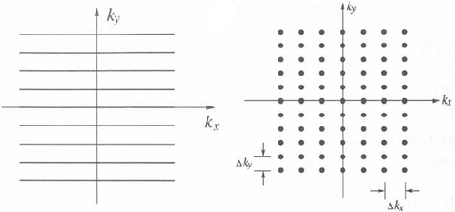
In MRI, two domains are involved: the data domain (the k-space) and the image domain. These domains are mutually related through the Fourier transform. In spin-echo MR experiments, the k-space is built-up row-wise and the raw data are sampled on a 2D rectangular trajectory as shown in figure 1. Let Ω be the grid of points fully covering the k-space: where Δk_x and Δk_y are FOV-dependent sampling intervals. Let D(nΔk_x, m Δk_y) be the k-space datum acquired at the grid point (nΔk_x, m Δk_y); the detected data form an N×M matrix D(k_x,k_y). Let I(x,y) be the N×M image reconstructed by a 2DIFT of the data matrix D(k_x,k_y): where,

Figure 1. k-Space sampling trajectory (left) and raw data matrix (right).

The represented MR image is the magnitude of I(x,y).

In a fast dynamic spin-echo MR experiment, the imaging time is decreased by collecting only the low spatial frequencies in the phase-encoded direction. Let Ω_low the grid points of the low sampled k-space:

A sequence of low sampled N_low×M data matrices D_t(k_x,k_y) defined as is acquired at T successive time instants. One or two fully encoded reference data sets are acquired on Ω; the reference data set D_B(k_x,k_y) acquired before the dynamic process is called baseline data set while the reference data set D_A(k_x,k_y) acquired after the dynamic process is called active data set. The baseline and active reference images I_B(x,y) and I_A(x,y) are reconstructed by a 2DIFT:

The acquired dynamic data sets D_t(k_x,k_y), t=1,…,T, are inverse Fourier transformed along the fully encoded horizontal direction.

Let be the data matrix D_t(k_x,k_y) transformed by DIFT along the rows: with , i=0,…,M-1. Since the number of phase-encodings is reduced from N to N_low, performing a DIFT along the vertical direction produces images with evident blurring in the phase-encoded direction.

A crucial point is that the dynamic image I_t(x,y) can be obtained by independently reconstructing each column of . In this way, the problem is reduced to the reconstruction of M signals of size N. Therefore, we present the reduced encodings methods only in the 1D case. For easier notation, in the following we omit the temporal index t and call and the point vectors in the data and in the image domain, respectively.

3. The algorithm

In this section, starting from the model-based framework proposed by 1, we deduce a general algorithm for the reconstruction of the high resolution dynamic MR signal I(x) from the undersampled data set D(k) with the use of a priori information.

The components of the unknown dynamic signal are the ideal values of a continuous dynamic function at the points x_j:

The unknown dynamic function can be factorized as: (2)

The functions and are called additive and multiplicative factors, respectively. These factors are assumed to be known and are used in (2) as additive and multiplicative constraints containing the a priori information on the uncollected high spatial frequencies content of the k-space. The function is called dynamic factor; it is the unknown factor which accounts for the changes in the signal occurring during the dynamic evolution. The dynamic factor is represented by a parametric model as (3)

The number of terms of the sum is determined by the number of available information on the desired dynamic signal, i.e. the number of acquired k-space dynamic data. By substituting the representation (3) for , equation (2) becomes: (4)

Equation (4) describes the wide class of the model-based reduced encodings methods where every continuous dynamic signal is uniquely determined by the model parameters . It is evident that a large variety of methods can be derived from equation (4) simply by choosing different factors and and basis functions φ_ℓ(x) and by using different methods for estimating the model parameters α_ℓ.

A representation of the high resolution signal I(x) is obtained by discretizing (4) at the N points x_j. Hence, the problem of reconstructing I(x) from the low resolution dynamic data set D(k) is converted to a coefficients estimation problem. In particular, the parameter estimation problem is solved in two steps: first the low resolution version of the dynamic factor is determined and then an interpolation problem is solved.

Let us consider the low resolution version of I(x), ; for , equation (2) becomes: (5) where .* indicates the element-wise product and the low resolution discrete factors , , and contain the values of , , and at the points , respectively. By applying the DFT to both the terms of (5), we obtain the expression (6) where ⊗ represents the convolution product. In matrix form: where is a matrix with a block Toeplitz structure: (7)

Therefore, given D₊(k) and D_*(k), the unknown vector D_d(k) is obtained by solving the linear system (8)

Since is relatively small (typically of size 64×64) and has Hermitian Toeplitz structure, the system (8) can be solved efficiently. In practice, may be severely ill-conditioned 2; in this case, some regularization is required for computing a useful solution of (8) without dominant noise. For example, the Truncated Singular Value Decomposition, the Lavrent'yev regularization method and Conjugate Gradient type iterative methods can be used efficiently (2 and references therein). A comparison of the results obtained with these methods is presented in 2.

Given D_d(k), then:

The next step consists in calculating the model coefficients α_ℓ. The coefficients estimation problem is solved as an interpolation problem: the coefficients are determined such that the continuous function interpolates the sample points : (9)

Using (3), relation (9) becomes (10) where the coefficient matrix is the matrix of the basis functions φ_ℓ sampled at the points . Summarizing, the computation of the coefficients α_ℓ requires the solution of the linear system (8) for determining and the solution of the linear system (10).

When the coefficients are determined, the high resolution dynamic factor I_d(x) can be computed from the parametric model (3); i.e. (11) where Φ is the basis functions matrix whose columns are the vectors

Now, the desired high resolution dynamic signal I(x) can be computed from (2): (12) where I₊(x) and I_*(x) are the high resolution discrete factors.

The algorithm of the presented unifying model-based method for dynamic MRI is the following:

Algorithm 1 Unifying model-based algorithm for dynamic MRI.

Input: dynamic data D(k)

additive factor I₊(x)

multiplicative factor I_*(x)

basis functions

Output: dynamic signal I(x)

Step 1 Compute the spectra D₊(k) and D_*(k) and the matrix .

Step 2 Compute D_d(k) by solving the linear system

Step 3 Compute the low resolution dynamic factor :

Step 4 Compute the basis functions matrix and compute the model coefficients vector α by solving the linear system:

Step 5 Compute the basis functions matrix Φ and compute the high resolution dynamic factor I_d(x):

Step 6 Compute the high resolution dynamic signal I(x):

We conclude this section with a remark on the solution of the general equation (4). In 1, equation (4) is solved with respect to the coefficients α_ℓ by fitting to the measured data. No further discussion is given in 1 on the solution of (4). We observe that the mere data-consistency requirement leads to the linear system (13)

The matrix A is such that (14) where is defined in (7) and is obtained as (15) where the DFT is applied to each column of . A detailed description of the derivation of (13) can be found in 3. The solution of (13) replaces Steps 2–4 of Algorithm 1.

The computational cost of this “direct” approach for computing α is due to the N_low DFTs in (15), the operations required by the matrix--matrix product (14) and the operations to solve (13) with the LU factorization. The computational cost of Steps 2–4 of Algorithm 1 is given by the cost of the solution of two linear systems (Steps 2 and 4), i.e operations, and by the cost of the DFT in Step 3. If the basis functions have compact support, then is sparse; for example, with cubic B-splines is a band diagonal matrix. In this case, the computational cost of Step 4 can further be reduced. Thus, Algorithm 1 is computationally more efficient than the direct approach (13). In addition, the authors' experience indicates that, in practice, A has a higher conditioning number than and is well-conditioned for a proper choice of the basis. These considerations indicate that performing Steps 2–4 of Algorithm 1 is preferable to solving (13).

4. Numerical methods

In this section, we derive new methods using B-spline basis functions and regularization. In the unifying model (4) the dynamic factor is represented in terms of continuous basis functions φ_ℓ(x).

The Fourier basis is chosen as a basis for MR images representation in 1,4–7; it uses a set of complex exponential functions defined as

In this case, the coefficient vector α is simply computed by (16) and I_d(x) is obtained by applying a DIFT to the zero-filled spectrum: (17) where indicates the zero-padded N ×1 data vector. Hence, with the Fourier basis, Steps 3–5 of Algorithm 1 are replaced by two discrete Fourier transforms. However, even if the Fourier basis is computationally advantageous, the DIFT of a zero-padded vector yields a signal with Gibbs artifacts degrading the quality of the reconstruction.

Different basis functions can be used in the previous model, such as B-spline functions. Because of their compact support and other attractive numerical properties (fast evaluation of individual B-spline functions by a recursion relation, band-structured matrix of values, …), the B-splines are a good choice for the interpolation problem. B-spline interpolation is accurate and has a relatively low computational cost. Therefore the use of a B-spline basis is proposed as a valid alternative to the usual Fourier basis in MR signal representation. In addition, a regularization procedure is introduced into the B-spline coefficients computation in order to reduce noise and artifacts in the reconstructed dynamic signal. The use of a regularization method in the computation of the model parameters α_ℓ is a further advantage of the B-spline basis over the classic Fourier basis.

When the B-splines are introduced as basis functions, the coefficients α_ℓ are determined by the linear system of equations (10) arising from the interpolation conditions. If the B-spline knot partition satisfies the Schoenberg--Whitney conditions 8, the coefficient matrix is nonsingular and the interpolation problem (10) has a unique solution α. The coefficient matrix is always a band diagonal matrix of bandwidth q, where q is the B-spline order.

Two different approaches to the solution of (10) are considered. In the first one, the linear system (10) is solved by a direct method. In the other case, a regularization method is used for computing the solution of the linear system (10). The rationale behind regularizing the model coefficients can be explained as follows. The dynamic function can be viewed as a parametric curve; in Computer Aided Geometric Design, the coefficients α_ℓ of the B-splines are called control points and the polygon obtained by connecting the adjacent control points is termed as control polygon. The B-splines serve the role of shape functions. The B-spline curve lies in the convex hull of its control polygon and its shape is defined and manipulated by the set of control points. The local support property of the B-splines implies that a change in a control point only affects a limited portion of the curve. These properties imply that the resulting curve is a smooth approximation of the control polygon and that the shape of the curve is determined by the position of its control points. Conversely, the control polygon can be thought as an approximation of the N_low values of the curve. By computing the model coefficients through a regularization method, the entire curve is regularized by requiring that its control points α_ℓ take on a regular structure. Therefore, the use of a regularization technique to determine the coefficients vector α is not due to the ill-conditioning of the linear system (10) but rather to the need of imposing a constraint on the smoothness of its solution. Among the various regularization methods known in literature, we have considered Tikhonov regularization technique 9,10. Other regularization methods can be used such as iterative regularization methods 11–13. They are more suitable to solve large size systems, because of their low computational complexity. In our case, we remark that many small size systems (of order N_low) must be solved. Moreover, our experience indicates that Tikhonov regularization performs better for dynamic MRI applications 13.

When Tikhonov regularization method is used, the coefficients vector α is estimated by solving the unconstrained optimization problem (18)

Since MR signals are characterized by edges in connection of the tissue boundaries, the matrix L is the first-order differential operator that better preserves such discontinuities in the reconstructed signal. The objective function of (18) is convex and it attains its minimum at the solution of the Euler--Lagrange equations: (19)

The coefficient matrix is symmetric and positive definite; therefore, (19) is efficiently solved by the Cholesky factorization. When the model coefficients are computed from (19), the resulting function is an approximate representation of the data because it does not exactly interpolate the sample values Finally, observe that solving (13) with Tikhonov method is not equivalent to (18) and is indeed less effective in reducing the Gibbs artifacts in the reconstructed signal.

Starting from the previous model (2), we consider two classes of methods: the Keyhole-like methods and the RIGR-like methods.

4.1. The Keyhole-like methods

The so-called Keyhole-like methods (from the Keyhole method 5–7,14, the technique commonly implemented on commercial systems for dynamic MRI) are obtained from (12) when the a priori information is provided by:

In this case, equation (12) becomes (20)

It immediately follows (21) hence, D_d(k) is determined without solving any linear system.

Different Keyhole-like methods are obtained from the general equation (20) according to the selected basis functions, the method used for computing the coefficients α_ℓ and the additive factor I₊(x). Possible choices of the additive factor are the following:

i.

The a priori information is provided by the high resolution baseline signal acquired before the dynamic process. If the Fourier basis is selected, equation (20) reduces to the classic KEYhole (KEY) method: the missing dynamic high frequencies are extrapolated from the spectrum DB(k) of the baseline signal and I(x) is reconstructed with a DIFT of the completed data vector. When the B-spline basis is employed, we obtain the B-spline KEYhole (BKEY) method with direct solution of (10) and the B-spline KEYhole method with Tikhonov regularization (BKEY_Tik).

ii.

where , t=1,…,T. The additive factor I+(x) of the t-th signal , t=1,…,T, of the temporal sequence is a weighted combination of the baseline and active reference signals. In this case, I+(x) depends on the time instant t. Then, at the beginning of the sequence, I+(x) is closer to IB(x) while, at the end of the sequence, I+(x) is closer to IA(x). In this way, I+(x) better approximates the temporal evolution of the “true” additive factor of the t-th unknown exact dynamic signal. According to the chosen basis, we obtain the Weighted KEYhole method (WKEY), the Weighted B-spline KEYhole method (WBKEY) with direct solution of (10) and the Weighted B-spline KEYhole method with Tikhonov regularization (WBKEY_Tik).

4.2. The RIGR-like methods

The Reduced-encoded Imaging by Generalized-series Reconstruction (RIGR)-like methods are similar to the RIGR method originally proposed by Liang and Lauterbur in 6 as an efficient technique for fast MRI. Successive developments of the RIGR method are the Two-references RIGR (TRIGR) 4 and the fast RIGR 15 methods.

The RIGR-like methods are obtained from the common equation (12) when the a priori information is encoded in the multiplicative factor and, eventually, in the additive factor; namely, when

Since , the linear system (8) has to be solved in order to compute D_d(k) and, consequently, . By choosing the Fourier basis or the B-spline basis and by selecting different factors I₊(x) and I_*(x), the various RIGR-like methods are obtained.

Possible choices of the factors are the following:

i.	and . With the Fourier basis, the classic RIGR method is obtained 6. If the B-spline basis is used, we obtain the B-spline RIGR (BRIGR) method with direct solution of (10) 3 and the B-spline RIGR method with Tikhonov regularization (BRIGR_Tik).
ii.	and . The dynamic factor represents the changes of the dynamic signal with respect to the baseline signal and the multiplicative factor encodes “difference” information into the model for I(x). According to the selected basis, the TRIGR method 4, the Two-references B-spline RIGR (TBRIGR) method with direct solution of (10) 3 and the Two-references B-spline RIGR (TBRIGR_Tik) method with Tikhonov regularization are obtained.
iii.	and , t=1,…,T. The multiplicative factor I*(x) of the t-th signal , t=1,…,T, of the temporal sequence is the absolute value of IW(t,x). According to the selected basis we obtain the Weighted RIGR (WRIGR) method, the Weighted B-spline (WBRIGR) RIGR method with direct solution of (10), and the Weighted B-spline RIGR method with Tikhonov regularization (WBRIGR_Tik).

The aforementioned numerical methods for dynamic MRI are further summarized in table 1.

Table 1. Summary of methods for dynamic MRI.

Class of the method	Method	Basis	I+(x)	I*(x)
Keyhole-like	KEY	Fourier	IB(x)	1
	BKEY	B-spline	IB(x)	1
	BKEY_Tik	Reg. B-spline	IB(x)	1
	WKEY	Fourier	IW(t,x)	1
	WBKEY	B-spline	IW(t,x)	1
	WBKEY_Tik	Reg. B-spline	IW(t,x)	1
RIGR-like	RIGR	Fourier	0	|IB(x)|
	BRIGR	B-spline	0	|IB(x)|
	BRIGR_Tik	Reg. B-spline	0	|IB(x)|
	TRIGR	Fourier	IB(x)	|IA(x)-IB(x)|
	TBRIGR	B-spline	IB(x)	|IA(x)-IB(x)|
	TBRIGR_Tik	Reg. B-spline	IB(x)	|IA(x)-IB(x)|
	WRIGR	Fourier	0	|IW(t,x)|
	WBRIGR	B-spline	0	|IW(t,x)|
	WBRIGR_Tik	Reg. B-spline	0	|IW(t,x)|

The application of the reconstruction methods to spin-echo images is immediate. In real MRI applications, a dynamic image I(x,y) has to be reconstructed from a dynamic data set undersampled along the phase-encoding direction. As explained in section 2, the horizontal direction of I(x,y) is first reconstructed by a DIFT and the matrix is obtained. Then, each column I(x,iΔy) is independently reconstructed by applying one of the described methods to .

5. Numerical experiments

In this section, we present the results obtained with the methods described in sections 4.1 and 4.2. We have considered test problems with both simulated and real MR data. In all the test problems, the Lavrent'yev regularization method has been used for solving the linear system (8); i.e. (8) is replaced by where γ is the regularization parameter.

In all the performed numerical experiments, we have chosen cubic B-splines as B-spline basis functions. The value of the regularization parameter λ of Tikhonov method (18) has been heuristically chosen, but it can be automatically selected by the L-curve or the Generalized Cross Validation criteria 10.

5.1. Simulated MR data

Two test problems with simulated MR data have been considered. The quality of the reconstructions is compared by means of the Root Mean Square Error (RMSE) and the Mean Absolute Error (MAE) defined as: where the M×N images I and are the reconstructed and the original images, respectively. Both RMSE and MAE measures compare two images on a pixel-by-pixel basis. The RMSE measure is very sensitive to a small number of pixels with very large intensity difference, while the MAE measure quantifies the mean of all the absolute pixel-by-pixel differences in I and .

5.1.1. Signal test problem

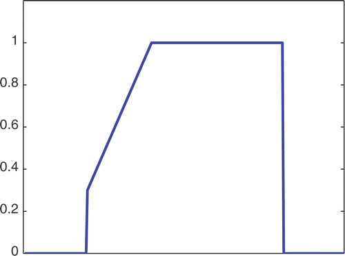
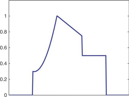
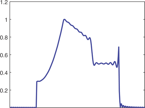
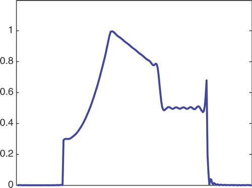
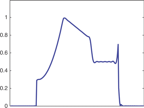
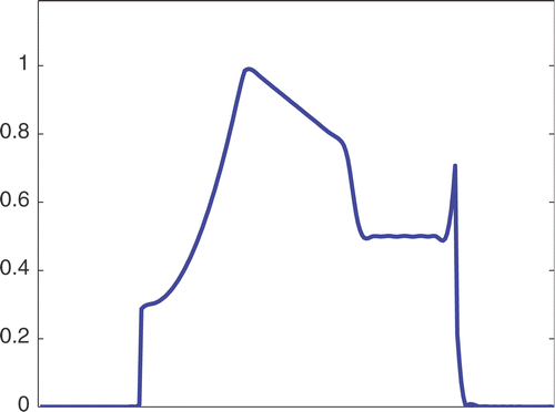
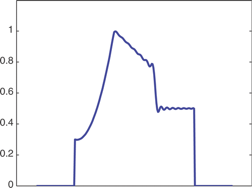
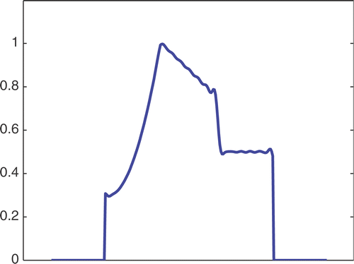
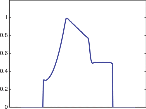
The first simulated test problem is a 1D test problem consisting in a reference signal I_B(x) (figure 2) and an exact dynamic signal (figure 3), both of N = 256 samples. The undersampling of the dynamic data is simulated by considering only a subset D(k) with the symmetric lowest frequencies of the spectrum of . The dynamic signals reconstructed with the Keyhole-like and RIGR-like methods are depicted in figures 4–7 and 8–11, respectively. In particular, figures 6–7 and 10–11 are obtained for different values of the regularization parameter λ. Table 2 shows the RMSE and MAE values. From the figures and the error measures, it is evident that the use of B-splines and regularization reduces the oscillations of both the Keyhole and RIGR methods. The use of regularization slightly smooths the peaks at the edges of the signal and, consequently, the RMSE measure of the BKEY_Tik and BRIGR_Tik methods is higher than that of the BKEY and BRIGR methods. Moreover, high values of λ greatly reduce the oscillations but the reconstructed signal is more smooth and the peaks are more rounded. Consequently, the corresponding error values increase, even if the plots look better. For this test problem .

Figure 2. Reference signal.

Figure 3. Dynamic signal.

Figure 4. KEY.

Figure 5. BKEY.

Figure 6. BKEY_Tikh (λ= 0.035).

Figure 7. BKEY_Tikh (λ = 0.1).

Figure 8. RIGR.

Figure 9. BRIGR.

Figure 10. BRIGR_Tikh (λ= 0.015).

Figure 11. BRIGR_Tikh (λ= 0.05).

Table 2. Error parameters for test problems with simulated MR data.

Test problem	Method	RMSE	MAE
Signal	KEY	0.021682	0.007900
	BKEY	0.020945	0.005759
	BKEY_Tikh (λ = 0.035)	0.023275	0.005564
	BKEY_Tikh (λ = 0.1)	0.025996	0.006459
	RIGR	0.009554	0.003128
	BRIGR	0.009356	0.002599
	BRIGR_Tikh (λ = 0.015)	0.010028	0.002589
	BRIGR_Tikh (λ = 0.065)	0.011760	0.002877
Circle	KEY	0.048053	0.035114
	BKEY	0.046493	0.032184
	BKEY_Tik	0.044949	0.026999
	RIGR	0.035362	0.019657
	BRIGR	0.034984	0.018877
	BRIGR_Tik	0.030785	0.013462

5.1.2. Circle test problem

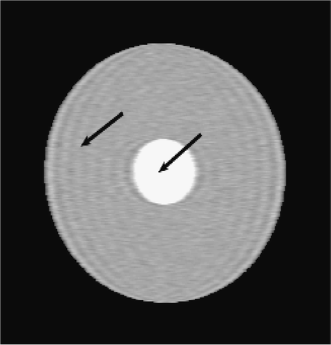
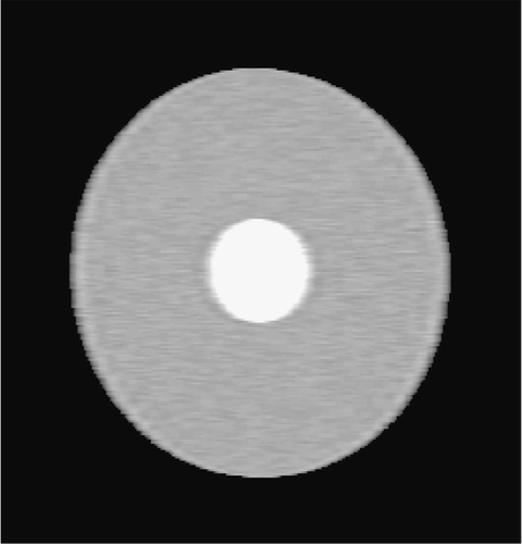
The second simulated test problem is the so-called circle test problem. This problem is used in the literature to represent the action of a contrast agent in the examined organ through the variations of gray levels in the dynamic image. Two images of size 256×256 represent the reference image I_B(x,y) and the exact dynamic image , respectively (figures 12 and 13). After Fourier transforming , a reduced scan spin-echo acquisition is simulated by considering the 64×256 (N_low = 64) dynamic lowest frequencies. White noise with has been added to the available dynamic frequencies. For this test problem, γ = 0.5.

Figure 12. Reference image.

Figure 13. Dynamic image.

Figures 14–16 and 17–19 show the reconstructions obtained with the Keyhole-like methods and with the RIGR-like methods, respectively. The Gibbs artifacts in the Keyhole reconstruction (figure 14) are reduced by the use of B-splines (figure 15) and further on by the use of regularization (figure 16); in any case an error (a white line) is evident near the border of the big circle. Among the RIGR-like methods (figures 17–19), the BRIGR method with regularization (figure 19) performs better and considerably reduces the noise and the errors near the border. The RMSE and MAE measures (table 2) confirm these considerations.

Figure 14. KEY.

Figure 15. BKEY.

Figure 16. BKEY_Tikh (λ= 0.03).

Figure 17. RIGR.

Figure 18. BRIGR.

Figure 19. BRIGR_Tikh (λ = 0.015).

5.2. Real MR data

5.2.1. Mouse test problem

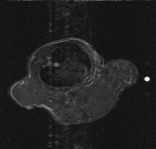
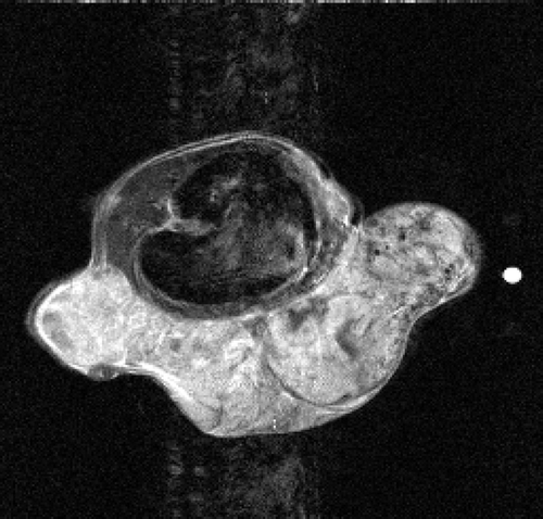
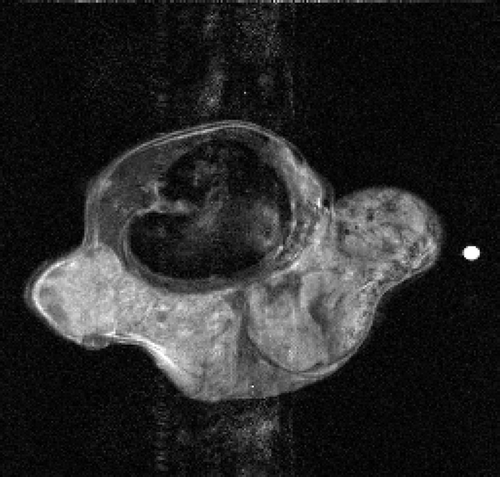
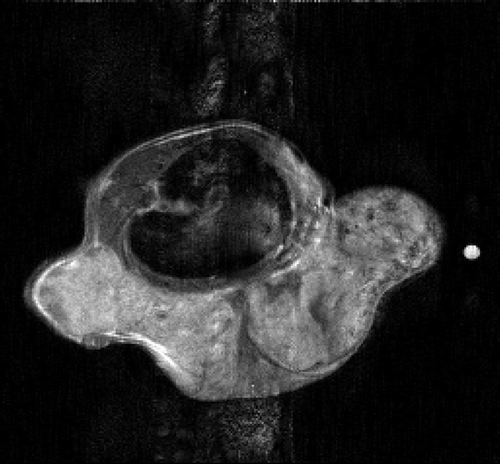
The real MR data of the mouse test problem have been downloaded from the site: http://mri.ifp.uiuc.edu/V/. They are constituted of six data sets from a mouse breast with a big tumor: a baseline reference data set and an active reference data set of 256 × 256 samples and four low-sampled dynamic data sets of 32× 256 samples, acquired by an MR spin-echo technique after injecting a contrast agent. The reference images and are shown in figures 20 and 21.

Figure 20. Baseline reference image .

Figure 21. Active reference image .

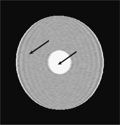
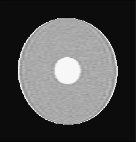
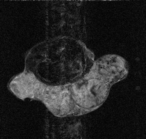
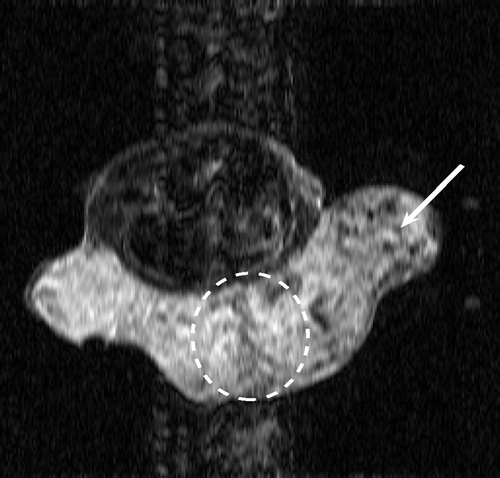
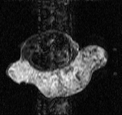
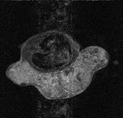
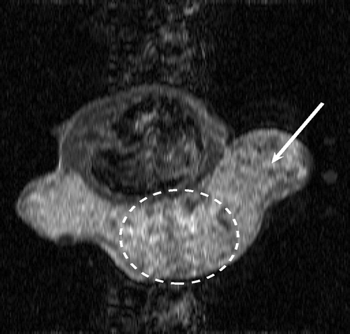
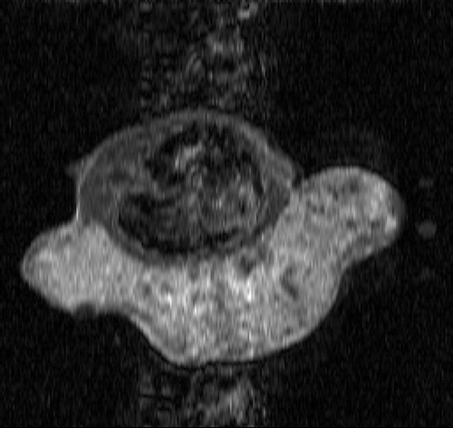
In the first set of performed tests, the active image has been used as an exact dynamic image and the described algorithms are applied to its 64× 256 (N_low = 64) lowest frequencies. In particular, the dynamic factor I_d(x) reconstructed with the presented methods is compared with the exact dynamic factor extrapolated from . Figures 22 and 26 show the exact dynamic factors. The results are shown in figures 23–25 and 27–29 for the Keyhole-like methods and the RIGR-like methods, respectively. The arrow and the white circle indicate the portions of the images where the Gibbs artifacts are more evident (figures 23 and 27). These artifacts are greatly reduced in the images represented with B-spline basis (figures 24 and 28) and regularization (figures 25 and 29).

Figure 22. Exact dynamic factor I_d(x) of Keyhole-like methods.

Figure 23. KEY dynamic factor.

Figure 24. BKEY dynamic factor.

Figure 25. BKEY_Tikh dynamic factor (λ = 0.03).

Figure 26. Exact dynamic factor I_d(x) of RIGR-like methods.

Figure 27. RIGR dynamic factor.

Figure 28. BRIGR dynamic factor.

Figure 29. BKEY_Tikh dynamic factor (λ = 0.03).

In order to show the effects with two reference images as a priori information, further tests have been performed on the data sets of the whole sequence. Figures 30–32 show the second image of the sequence obtained by the TBRIGR_Tik, WBKEY_Tik, and WBRIGR_Tik algorithms, respectively. We can conclude that even in this test problem with real MR data, the use of B-splines and regularization gives good results in terms of image quality.

Figure 30. TBRIGR_Tik (λ = 0.1).

Figure 31. WBKEY_Tik (λ = 0.1).

Figure 32. WBRIGR_Tik (λ = 0.1).

6. Conclusions

In this article, we have presented a numerical framework for fast dynamic MRI with the use of a priori information. We have also proposed the use of B-spline functions for the representation of MR signals and images and the use of regularization in the reconstruction process.

Two classes of methods have been considered in detail, the Keyhole-like methods and the RIGR-like methods. The methods have been tested both on simulated and real MR data. The Keyhole-like methods require a lower computational effort, but they produce Gibbs artifacts in the reconstructed images. The use of B-splines and regularization greatly reduces the artifacts and enhances the Keyhole performance, especially when two reference images are available. The RIGR-like methods perform well when the reference images are of very high quality; in any case, they are computationally more expensive than the Keyhole-like methods.

We conclude with a comment on the use of B-splines and regularization in Algorithm 1. A wide theoretical analysis existing in the literature (see, for example, 16–18) shows that B-splines are very efficient and accurate basis functions for medical image representation. Furthermore, the results of our numerical experiments confirm that B-splines perform well for MRI. These theoretical and experimental considerations justify the choice of B-spline basis functions. However, we underline that the presented approach, using B-spline basis functions and regularization can be extended to other non-Fourier basis functions φ_ℓ. Also in this more general case, the model coefficients vector α can be computed by solving the Tikhonov system (19) where is the basis functions matrix.

Acknowledgement

This work was supported by the italian MIUR project Inverse Problems in Medical Imaging 2004--2006 (Grant No. 2004015818).

References

- Tsao, J, Behnia, B, and Webb, G, 2001. Unifying linear prior-information-driven methods for accelerated image acquisition., Magnetic Resonance in Medicine 46 (2001), pp. 652–660.
- Loli Piccolomini, E, Zama, F, Zanghirati, G, and Formiconi, A, 2002. Regularization methods in dynamic MRI., Applied Mathematics and Computation 132 (2) (2002), pp. 325–339.
- Loli Piccolomini, E, Landi, G, and Zama, F, 2005. A B-spline parametric model for high resolution dynamic Magnetic Resonance Imaging., Applied Mathematics and Computation 164 (2005), pp. 133–148.
- Hanson, JM, Liang, ZP, Wiener, EC, and Lauterbur, PC, 1996. Fast dynamic imaging using two reference images., Magnetic Resonance in Medicine 36 (1996), pp. 172–175.
- Hu, X, 1994. On the “Keyhole” technique., Journal of Magnetic Resonance Imaging 4 (2) (1994), p. 231.
- Liang, ZP, and Lauterbur, PC, 1994. An efficient method for dynamic Magnetic Resonance imaging., IEEE Transactions on Medical Imaging 13 (4) (1994), pp. 677–686.
- van Vaals, JJ, Brummer, ME, Dixon, WT, Tuithof, HH, Engels, H, Nelson, RC, Gerety, BM, Chezmar, JL, and Den Boer, JA, 1993. “Keyhole” method for accelerating imaging of contrast agent uptake., Journal of Magnetic Resonance Imaging 3 (1993), pp. 671–675.
- Schumaker, LL, 1981. Spline Functions: Basic Theory. New York: John Wiley and Sons, Inc.; 1981.
- Groetsch, CW, 1984. "Theory of Tikhonov regularization for Fredholm equations of the first kind.". In: Pitman Reserch Notes in Mathematics Series. London: Longman; 1984.
- Hansen, PC, 1997. Rank-Deficient and Discrete Ill-Posed Problems. Philadelphia: SIAM; 1997.
- Calvetti, D, Lewis, B, and Reichel, L, 2001. On the choice of subspace for iterative methods for linear discrete ill-posed problems., International Journal of Applied Mathematics and Computer Science 11 (2001), pp. 1069–1092.
- Hanke, M, 1995. "Conjugate gradient type methods for ill-posed problems.". In: Pitman Reserch Notes in Mathematics Series. Harlow, UK: Longman; 1995.
- Landi, G, and Loli Piccolomini, E, 2005. Numerical methods for dynamic Magnetic Resonance imaging. Technical report, Almae Matris Studiorum Acta (2005), August 2005. http://amsacta.cib.unibo.it/.
- Jones, RA, Haraldseth, O, Muller, TB, Rinck, PA, and Oksendal, AN, 1993. K-space substitution: a novel dynamic imaging technique., Magnetic Resonance in Medicine 29 (1993), pp. 830–834.
- Liang, ZP, Madore, B, Glover, GH, and Pelc, NJ, 2003. Fast algorithms for GS-model-based image reconstruction in data-sharing Fourier imaging., IEEE Transactions on Medical Imaging 22 (8) (2003), pp. 1026–1030.
- Lehmann, TM, Gonner, C, and Spitzer, K, 1999. Survey: interpolation methods in medical image processing., IEEE Transactions on Medical Imaging 18 (11) (1999), pp. 1049–1075.
- Meijerring, EHW, Niessen, WJ, and Viergever, MA, 2001. Quantitative evaluation of convolution-based methods for medical image interpolation., Medical Image Analysis. 5 (2001), pp. 111–126.
- Unser, M, 1999. Splines: a perfect fit for signal and image processing., IEEE Signal Processing Magazine 16 (1999), pp. 22–38.