Inverse problems explicit and implicit formulations with applications in engineering, biophysics and biotechnology

Abstract

In this work, we present a few explicit and implicit formulations used in the analysis and solution of inverse problems. These formulations have been developed and/or applied by the authors to the solution of different problems with applications in engineering, biophysics and biotechnology. Here emphasis is given to a matrix-based explicit formulation, and to the construction of a generalized family of regularization terms which is used when the inverse problem is formulated implicitly as an optimization problem. The efficacy of the methodologies developed is demonstrated with the results for a few test cases using noiseless and noisy synthetic data.

Keywords:

• Inverse problems
• Explicit formulations
• Implicit formulations
• Matrix-based formulation
• Tikhonov's functional
• Bregman distances

1. Introduction

Due to several relevant applications, an ever growing interest towards the formulation and solution of inverse problems in engineering has been observed in recent years. Their applications extend beyond the usual engineering practice field into other areas of human activity such as medicine and biophysics.

Inverse problems are formulated in many different ways, and may be classified in two groups: explicit and implicit formulations 1,2.

In order to show a few explicit and implicit formulations in this work, we have chosen applications involving inverse radiative-transfer problems.

Among the explicit formulations we give emphasis to an analytical matrix-based formulation 3.

With respect to the implicit formulations, in most cases the inverse problem is formulated as an optimization one, and the focus of the solution approach is then moved to the use of deterministic, stochastic or hybrid methods for a cost function minimization 4–9. Other heuristics such as Artificial Neural Networks, and their hybridization with other methods are also used 10,11. In such cases regularization often plays an important role, and special attention is then devoted to the construction of the regularization terms 12–14.

In the present work, we derive and implement a family of regularization terms based on Bregman distances constructed with moments of the q-discrepancy 15, and minimize the Tikhonov's regularization functional with a gradient-based method.

The main ideas and results presented in this article extend the work previously performed by the authors with applications in engineering, biophysics, and biotechnology: (i) non-destructive testing in engineering 2–4,6,8–11,16–19; (ii) parameter estimation in biotechnological processes involving the adsorption of biomolecules 7; (iii) restoration of biological images acquired in nanoscale with Atomic Force Microscopes 12–14; and (iv) computerized tomography 20.

2. Pseudo-explicit and explicit formulations for inverse problems

Inverse problems may be formulated either explicitly or implicitly 1,2. In the former, the equations used for the modeling of the direct problem are manipulated, and then in the resulting formulation of the inverse problem the unknowns to be determined appear explicitly.

2.1 Source-detector methodology

Roberty and Silva Neto with co-workers 16–20 have proposed and developed the source-detector methodology for the solution of inverse radiative-transfer problems. The direct problem of the interaction of radiation with a one-dimensional participating media of thickness L is mathematically modeled with the linear version of the Boltzmann equation 21,22 (1) (2) where φⁱ(x, μ) represents the radiation intensity, i is the index for a particular boundary condition, either at the boundary surface x_b = 0 or x_b = L, indicating a specific direction represented by μ_i, at which an external source of collimated radiation is located, μ is the cosine of the polar angle, σ_t is the total extinction coefficient, i.e., absorption plus scattering, σ_s is the scattering coefficient, S represents a distributed internal source, and f is the intensity of the external source.

The inverse problem solved in 16–19 consisted of estimating the radiative properties σ_t and σ_s using the information on the intensity of the exit radiation acquired with external detectors. Problem (1) is referred to as the source problem. An adjoint problem is then written, using reference values for the unknowns, i.e., being denominated the detector problem. The solution of the detector problem is represented by φ*^j, and the index j represents the location μ_j at which a detector is located, at either of the boundary surfaces, i.e., x_b = 0 or x_b = L. Equation (1a) is then multiplied by the solution of the adjoint problem φ*^j(x, μ) and the resulting expression is integrated over the spatial and angular domains, i.e., x = [0, L] and μ = [−1, 1], respectively. The resulting equation is integrated by parts and the formulation of the adjoint problem is introduced in the resulting expression yielding 16 (3)

Equation (2) represents in fact a system of nonlinear equations in which for each location of a source, indicated by the index i, and for each location of a detector, indicated by the index j, one equation is written. The experimental data on the exit radiation intensities is used in the term on the right-hand side of the equation. The unknowns σ_t and σ_s are explicitly represented in the formulation of the inverse problem (2). From equation (2), we see that the internal distributed source, S, may also be considered unknown, and the respective reference value is represented by S^R.

These reference values in equation (2) are considered previously known. Therefore, the inverse problem here described consists of determining deviations from such reference values. Just to give an example, consider the computerized tomography inverse problem in which we look for the value of σ_t for a biological sample which could be different from the previously known value for a healthy tissue.

Observe that in the source-detector methodology described here, the solution of the direct problem (1) which depends itself on the values of the unknowns, i.e., is required. In the iterative procedure constructed for the solution of the system (2) we lag the values of φⁱ by using the coefficients σ_t and σ_s calculated at the previous iteration. For this reason, we classify the source-detector methodology presented in this section as a pseudo-explicit inverse problem formulation.

Further details of the method and numerical results can be found in 16–20.

2.2 Analytical solution based on the moments of the exit radiation intensity

McCormick and Silva Neto 2,23 proposed and developed an explicit formulation for an inverse radiative-transfer problem in one-dimensional participating media which does not require the solution of the direct problem.

The dimensionless mathematical formulation for the direct radiative-transfer problem with azimuthal symmetry in a plane-parallel, gray, isotropically scattering slab of optical thickness τ₀, with diffusely reflecting boundaries, and subjected to external isotropic illumination at both boundaries, τ = 0 and τ = τ₀, is given by 22: (4) (5) (6) where I(τ, μ) is the dimensionless radiation intensity, τ is the optical variable, μ is the direction cosine of the radiation beam with the positive τ axis, ω is the single scattering albedo, ρ₁ and ρ₂ represent the diffuse reflectivities at the inner part of the boundary surfaces, and f₁(μ) and f₂(μ) are the strengths of external radiation sources at the boundaries τ = 0 and τ = τ₀, respectively.

The inverse problem solved in 2,23 consisted in estimating ρ₁, ρ₂, and ω, using as experimental data the exit radiation intensities measured by external detectors in two different experiments.

In the first experiment isotropic illumination is used, i.e., f₁(μ) = A₁ = constant and f₂(μ) = A₂ = constant, and the exit radiation intensities I_eff(0, −μ) and I_eff(τ₀, μ) are measured, with μ > 0. From the experimental data, the following moments are written: (7) (8) and the boundary conditions given by equations (3b–3c are then written as (9) (10)

The procedure to derive the formulation of the inverse problem described here is based on the ideas developed by Siewert 24,25 and McCormick 26. The details of the derivation can be found in 23, and will not be repeated in the present work. By manipulating equation (3a) and introducing equations (4) and (5), two nonlinear equations are obtained (11) where (12) (13) (14) (15) (16)

We want to obtain estimates for three unknowns, ρ₁, ρ₂, and ω, but only two equations (equation 6(a, b)), are available so far. The third equation is obtained from the manipulation of equation (3a), and from a second experiment in which f₁(μ) = C₁/μ is used in equation (3b), where C₁ is a constant, and f₂(μ) = 0 in equation (3c). Using the new set of experimental data represented by with μ > 0, and the respective moments calculated with equation (4a, b), yielding with n = 0, 1, 2, the boundary conditions are written as (17) (18)

The third inverse equation is then obtained from the manipulation of equation (3a), also equation (8a, b) being introduced, resulting in (19) where (20) (21)

Equations (6a, b) and (9) are sufficient, in principle, to determine the three unknowns ρ₁, ρ₂, and ω. Note that these equations involve a highly nonlinear search. Nonetheless, the unknowns appear explicitly represented, and therefore we classify this inverse problem formulation as an explicit one. Observe also that it does not require the solution of the direct problem.

Further details of the method and numerical results can be found in 2,23.

2.3 Explicit matrix formulation

2.3.1 Direct problem

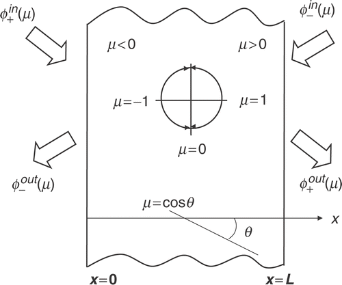
Consider the radiative-transfer problem in the absorbing and anisotropic scattering plane-parallel gray medium of thickness L represented in figure 1.

Figure 1. One-dimensional plane-parallel participating medium.

The mathematical description of the radiation interaction with the participating medium is given by the linear version of the Boltzmann equation, which for the case of azimuthal symmetry is written as 3 (22) (23) (24) where φ(x, μ) represents the radiation intensity, x is the spatial coordinate, μ is the cosine of the polar angle, σ_t is the total extinction coefficient, σ_s is the scattering coefficient (σ_sl, l = 0, 1, … , M, corresponding to the expansion coefficients of the phase function of anisotropic scattering in normalized Legendre polynomials, with a total number of M + 1 coefficients), p_l represents the normalized Legendre polynomials, and represent the intensity of the incoming radiation at x = 0 and x = L, respectively.

Equation (11a) may be written as (25) where T is the multiplicative operator, i.e., (26) and A_c is the collision operator, i.e., (27)

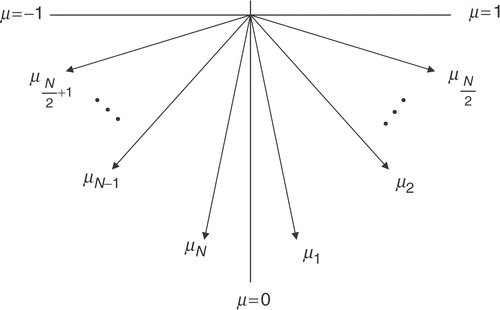
Considering the discretization of the angular domain represented in figure 2, and defining (28) (29) the solution of equation (12a) is given by (30) where x₀ represents the location at which the radiation comes into the medium.

Figure 2. Discretization of the angular domain.

Observe that due to the discretization of the angular domain, represented schematically in figure 2, the multiplicative operator appearing in equation (12a, b) is now replaced by a diagonal matrix, as shown in equation (14). Also as the node zero is avoided in the discretization, T is invertible.

Being the matrix (31) invertible and diagonalizable 27, we may obtain a diagonal matrix T_λ such that (32)

The diagonal entries of T_λ are the eigenvalues of B⁻¹, and F is a unitary matrix.

From equations (16) and (17) we obtain (33) (34) and (35)

2.3.2 Inverse problem

We are here interested in estimating the total extinction coefficient σ_t and the coefficients σ_sl, l = 0, 1, … , M, of the expansion of the anisotropic phase function in normalized Legendre polynomials.

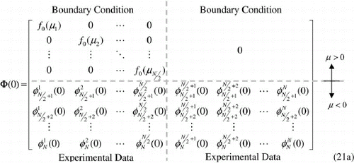
We construct a set of N experiments in which for each experiment k, with k = 1, 2, … , N, we apply the boundary condition (36) (37)

We then construct the following matrices Φ(0) and Φ(L) by properly arranging the available information of boundary condition (radiation coming into the medium at τ = 0, with μ > 0, i.e., f₀(μ), and at τ = τ₀, with, μ < 0, i.e., f_L(μ)) and exit radiation intensities ( for μ < 0, and for μ > 0, with i = 1, 2, … , N and k = 1, 2, … , N),

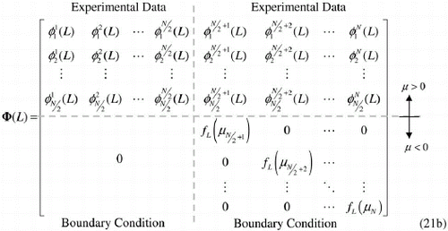
Using x = L and x₀ = 0 in equation (15), we write (38)

Defining the transmission operator T_r such that (39) we write (40)

From equations (18b), (23) and (24) we obtain (41) which results in (42) where D is a diagonal matrix.

If Φ(0) is invertible, we obtain from equations (24) and (26), (43)

On defining (44) we get from equations (23) and (27), (45)

Using a Gaussian quadrature in the last term of the right-hand side of equation (11a) with the collocation points μ_i, i = 1, 2, … , N, represented in figure 2, and the weights of the quadrature a_i, i = 1, 2, … , N, equation (12a) is rewritten as (46) where (47)

The elements of matrix A_c are (48) such that (49)

Using the Fourier–Legendre series (50) the orthogonality condition (51) and knowing that (52) Equation (33) may be written as (53)

Truncating the second summation in equation (37) at l = M₁, with M₁ > M, and defining the matrices (54) (55) we write (56)

From equations (28), (29), and (40) we obtain (57) and therefore (58)

The values of σ_sl decrease with the increasing value of l, and also σ_sl = 0 for l > M. Therefore, from the higher-order terms we obtain the estimated value for σ_t, and we are then able to estimate the values of σ_sl for the lower-order terms, i.e., l ≤ M.

Using the known boundary conditions and the measured values for the intensity of the exit radiation, properly arranged in matrices Φ(0) and Φ(L), matrices F and D are calculated, and then estimates for the unknowns σ_t and σ_sl, with l = 1, 2, … , M, are directly obtained from equation (42).

As the unknowns appear explicitly in the formulation of the inverse problem, this formulation is classified as an explicit one. Observe that the solution of the direct problem is not required.

3. Implicit formulations for inverse problems

When formulated implicitly inverse problems usually require the minimization of a cost functional associated with the squared residues between an observable quantity, i.e., a quantity that can be measured, and the calculated value for such quantity 2.

As inverse problems are usually ill-posed, or at least ill-conditioned, they are affected by the noise that is always present in the experimental data.

An effective strategy to solve such problems is to replace the original inverse problem of interest by another one that is close to the former, but is less affected by the experimental data noise. Such an approach was clearly structured by Tikhonov 28. In Tikhonov's approach, a regularized functional is developed, in which an extra term, that may include some prior information related to the unknowns to be estimated, is added to the original objective functional to be minimized. Several published papers 29–32 are related to the use, analysis and proposition of Tikhonov's regularization terms.

For the minimization of the original cost functional, or the Tikhonov's regularization functional, several methods may be used, being either deterministic 4,8 or stochastic methods 5,7. Hybrid approaches combining deterministic and stochastic methods have also been used 6,9, as well as other heuristics such as Artificial Neural Networks 10,11.

In this section, we focus on the proposition and use of a two-parameter family of regularization terms for Tikhonov's functional. For the cost functional minimization, a deterministic gradient-based method is used.

3.1 Mathematical formulation of the direct and inverse problems

We consider here the radiative-transfer problem described in section 2.2, whose mathematical formulation is given by equation (3a–c).

When the boundary conditions and the material properties are known, one has the so-called direct problem, mathematically modeled by equation (3a–c), which can be solved yielding the values of the radiation intensity I(τ, μ), for every point in the spatial and angular domains, i.e., 0 ≤ τ ≤ τ₀ and −1 ≤ μ ≤ 1. As will be presented next, in the approach described in this section for the solution of the inverse problem, the solution of the direct radiative-transfer problem is required. We then use Chandrasekhar's discrete ordinates method 33 combined with the finite difference method for that purpose.

The inverse problem we are interested in consists of estimating the optical thickness τ₀, the single scattering albedo ω, and the diffuse reflectivities ρ₁ and ρ₂. As these radiative properties cannot be measured directly, experimental data on the intensity of the exit radiation at τ = 0 and τ = τ₀ are measured at different polar angles, and using this information we try to solve the inverse problem. Therefore, by using the measured data Y_i, i = 1, 2, … , N_d, where N_d is the total number of experimental data available, we want to determine the vector of unknowns defined as (59) where the superscript T indicates transpose.

As the number of experimental data N_d, is usually much larger than the number of unknowns N_u (here N_u = 4), we formulate the inverse problem as a finite dimensional optimization problem, in which we seek to minimize the Tikhonov's regularization functional (60) where represents the calculated values for the exit radiation intensity obtained using an estimate for the vector of unknowns α is the regularization parameter, Γ is the regularization term, and is a vector with reference values (prior information) for the unknowns.

In the formulation of the inverse problem presented in this section, the unknowns appear implicitly in the first term on the right-hand side of equation (44). For this reason, we classify it as an implicit inverse problem formulation.

3.2 General regularization term

Cidade et al. 12–14 constructed a one-parameter family of regularization terms for the solution of the inverse problem of atomic force microscopy image restoration, with applications in biophysics. These regularization terms are in fact Bregman distances 34 constructed with the q-discrepancy functional which is a particular case of Csiszár's measure 35,36.

Carita Montero et al. 37 used the same one-parameter family of functions as the cost functional to be minimized in an inverse problem in computerized tomography.

Berrocal Tito et al. 38 developed and implemented a family of Bregman distances constructed with moments of the q-discrepancy 15 either as regularization terms or the cost functional to be minimized in an inverse problem of parameter estimation for an environmental model.

In the present work we use Bregman distances 34, constructed with moments of the q-discrepancy 15,35,38, as the regularization terms Γ in equation (44), in order to estimate the vector of unknowns given by equation (43) considering that reference values for the unknowns, are available, as well as the experimental data on the intensity of the exit radiation, Y_i, with i = 1, 2, … , N_d.

The m-th order moment of the q-discrepancy is defined as (61) where N_u, as aforementioned, is the total number of unknowns in the inverse problem we want to solve, i.e., N_u = 4. The functional η_m,q represents the deviation of each radiative property of the medium p_i raised to the power q, with respect to an expected value. The parameter q is a real positive number.

When q → 0 the entropy functional is obtained (62)

The Bregman distances may be derived considering the second and higher-order terms in a Taylor's expansion, resulting in (63) where η( ·) is a Bregman function.

Introducing equation (45) into equation (47), results (64) which for the particular case q → 0 yields (65)

Using the Bregman distances as the regularization terms in Tikhonov's functional, we obtain from equations (44) and (48), (66) where the elements of the vector of residues are given by (67)

3.3 Solution of the inverse problem

In order to find the estimated values of the unknowns which minimize the Tikhonov's functional given by equation (50), we first write the critical point equation (68) leading to (69) where the elements of the Jacobian matrix are given by (70) and (71)

Writing the Taylor's expansions and keeping only the terms up to the first order (72) (73) where n will soon become the iteration index for the iterative procedure that will be constructed for the determination of the new estimates for the unknowns, with (74) and introducing equations (56) and (57) into equation (53), results (75) where the elements of the Jacobian matrix J_D are given by (76)

The first and second derivatives of the Bregman distances constructed with the moments of the q-discrepancy which will be necessary in equations (55) and (60), and consequently in equation (59), are given, for the case q > 0, by (77) (78) and for the limit case when q → 0 by (79) (80)

For the solution of the inverse problem we start with an initial guess and then new estimates are obtained from equation (58) with the corrections being obtained from the solution of the system of linear algebraic equations (59).

The iterative procedure is interrupted when a stopping criterion is satisfied, e.g., (81) where ϵ is a tolerance, say 10⁻⁵.

4. Results and discussion

As the main objective of this work is to present the explicit matrix formulation described in section 2.3, and the implicit formulation with the family of regularization terms constructed with the Bregman distances described in section 3.2, in the next two sections the results obtained with these formulations are presented for inverse problems of radiative properties estimation.

4.1 Estimation of the scattering and extinction coefficients with the matrix-based explicit formulation

As real experimental data was not available, we generated synthetic experimental data by adding random noise to the calculated values of the radiation intensity (82) where r_i represents pseudo-random numbers chosen from a normal distribution with zero mean, and σ emulates the standard deviation of the measurement errors.

In order to demonstrate the feasibility of the explicit formulation developed we have chosen a slab of thickness L = 0.5 cm. As shown in table 1, four sets of exact values of the scattering coefficients σ_sl are considered and for each set three different values are used for the total extinction coefficient, namely σ_t = 0.5 cm⁻¹, 0.8 cm⁻¹, and 1.2 cm⁻¹, yielding a total of 12 test cases. Cases 1A–4A and 1C–4C represent high and low scattering media, respectively.

Table 1. Exact values of scattering (σ_sl) and extinction (σ_t) coefficients (cm⁻¹); L = 0.5 cm

Test case	Scattering coefficients	Extinction coefficients
1A	[0.4, 0.2, 0.1, 0.0, 0.0]	0.5
1B		0.8
1C		1.2
2A	[0.4, 0.2, 0.1, 0.05, 0.0]	0.5
2B		0.8
2C		1.2
3A	[0.4, 0.0647, 0.0431, 0.0080, 1.7E−6, 0.0]	0.5
3B		0.8
3C		1.2
4A	[0.4, −0.0754, 0.0238, 0.0049, 0.0004, 2.29E−5, 0.0]	0.5
4B		0.8
4C		1.2

In tables 2 and 3, the estimated values for the scattering σ_sl and extinction σ_t coefficients, respectively, are shown. We considered N = 12 for test cases 1 and 2, N = 14 for test case 3, and N = 16 for test case 4, in the angular domain discretization (figure 2) used for the discrete ordinates method. Experimental data with measurement errors up to 0, 5, 9.5, and 14% were also considered. These results are also presented in figures 3–6.

Figure 3. Estimated values for the scattering coefficients. Test case 1: (σ_sl = 0.4, 0.2, 0.1 and 0.0 cm⁻¹); L = 0.5 cm; N = 12. Error in experimental data: * = 0%; ∇ < 5%; × < 9.5%; and O < 14%. (a) Test case 1A: (σ_t = 0.5 cm⁻¹); (b) test case 1B: (σ_t = 0.8 cm⁻¹); (c) Test case 1C: (σ_t = 1.2 cm⁻¹).

Figure 4. Estimated values for the scattering coefficients. Test case 2: (σ_sl = 0.4, 0.2, 0.1, 0.05, and 0.0 cm⁻¹). L = 0.5 cm; N = 12. Error in experimental data: * = 0%; ∇ < 5%; × < 9.5%; and O < 14%. (a) Test case 2A: (σ_t = 0.5 cm⁻¹); (b) test case 2B: (σ_t = 0.8 cm⁻¹); (c) test case 2C: (σ_t = 1.2 cm⁻¹).

Figure 5. Estimated values for the scattering coefficients. Test case 3: (σ_sl = 0.4, 0.0647, 0.0431, 0.0080 and 1.7E-6 cm⁻¹). L = 0.5 cm; N = 14. Error in experimental data: * = 0%; ∇ < 5%; × < 9.5%; and O < 14%. (a) Test case 3A: (σ_t = 0.5 cm⁻¹); (b) test case 3B: (σ_t = 0.8 cm⁻¹); (c) test case 3C: (σ_t = 1.2 cm⁻¹).

Figure 6. Estimated values for the scattering coefficients. Test case 4: (σ_sl = 0.4, −0.0754, 0.0238, 0.0049, 0.0004, 2.29E−5, 0.0 cm⁻¹). L = 0.5 cm; N = 16. Error in experimental data: * = 0%; ∇ < 5%; × < 9.5%; and O < 14%. (a) Test case 4A: (σ_t = 0.5 cm⁻¹); (b) test case 4B: (σ_t = 0.8 cm⁻¹); (c) test case 4C: (σ_t = 1.2 cm⁻¹).

Table 2. Estimated values for the scattering coefficients, σ_sl(cm⁻¹); L = 0.5 cm. (EED: error in experimental data; PRE (%): percentage relative error = )

Test case	EED = 0%	PRE(%)	EED < 5%	PRE(%)	EED < 9.5%	PRE(%)	EED < 14%	PRE(%)
(a) Test cases 1 and 2 (N = 12)
1A	0.400	0.000	0.400	0.006	0.400	0.011	0.400	0.017
	0.200	0.000	0.200	0.967	0.200	1.936	0.200	2.912
	0.100	0.000	0.101	7.602	0.101	15.26	0.102	22.96
1B	0.400	0.000	0.400	0.069	0.401	0.137	0.401	0.202
	0.200	0.000	0.201	0.685	0.203	1.368	0.204	2.049
	0.100	0.000	0.107	6.865	0.114	13.74	0.121	20.63
1C	0.400	0.000	0.400	0.052	0.400	0.104	0.401	0.155
	0.200	0.000	0.200	0.152	0.201	0.303	0.201	0.454
	0.100	0.000	0.102	2.144	0.104	4.286	0.106	6.427
2A	0.400	0.000	0.400	0.007	0.400	0.013	0.400	0.020
	0.200	0.000	0.202	1.073	0.204	2.149	0.207	3.232
	0.100	0.000	0.108	8.421	0.117	16.91	0.126	25.45
	0.050	0.000	0.046	7.887	0.042	15.73	0.038	23.54
2B	0.400	0.000	0.400	0.067	0.401	0.132	0.401	0.195
	0.200	0.000	0.201	0.655	0.203	1.308	0.204	1.960
	0.100	0.000	0.107	6.546	0.113	13.10	0.120	19.67
	0.050	0.000	0.047	5.377	0.045	10.74	0.042	16.10
2C	0.400	0.000	0.400	0.060	0.401	0.119	0.401	0.178
	0.200	0.000	0.200	0.174	0.201	0.347	0.201	0.520
	0.100	0.000	0.103	2.446	0.105	4.889	0.107	7.329
	0.050	0.000	0.049	1.439	0.050	2.879	0.048	4.320
(b) Test case 3 (N = 14)
3A	0.40	0.000	0.398	0.401	0.397	0.706	0.396	0.992
	0.0647	0.000	0.063	9.364	0.052	19.01	0.048	26.27
	0.0431	0.000	0.079	83.85	0.116	168.3	0.152	251.4
	0.008	0.000	0.020	152.0	0.030	280.3	0.039	392.9
	1.78e−6	0.000	0.039	2.2e6	0.076	4.3e6	0.112	6.3e6
3B	0.40	0.000	0.398	0.631	0.395	1.252	0.393	1.862
	0.0647	0.000	0.063	2.519	0.061	5.338	0.059	8.381
	0.0431	0.000	0.059	36.03	0.074	71.86	0.089	107.5
	0.008	0.000	0.013	63.39	0.018	122.9	0.022	178.8
	1.78e−6	0.000	0.017	9.5e5	0.033	1.9e6	0.050	2.8e6
3C	0.40	0.000	0.399	0.163	0.399	0.325	0.398	0.487
	0.0647	0.000	0.065	0.3546	0.064	0.710	0.064	1.069
	0.0431	0.000	0.046	5.1	0.048	12.09	0.051	18.11
	0.008	0.000	0.009	9.913	0.010	19.75	0.010	29.50
	1.78e−6	0.000	0.003	1.6e5	0.006	3.2e5	0.008	4.7e5
(c) Test case 4 (N = 16)
4A	0.400	0.000	0.394	1.389	0.389	2.707	0.384	3.955
	−0.0754	0.000	−0.075	0.080	−0.075	0.532	−0.074	1.625
	0.0238	0.000	0.050	111.5	0.075	216.1	0.099	315.9
	0.0049	0.000	0.027	452.6	0.049	903.7	0.072	1358.2
	0.0004	0.000	−0.004	1175	−0.009	2459	−0.015	3817.6
	2.29e−5	0.000	−0.009	39965	−0.018	8030	−0.028	1.2e5
4B	0.400	0.000	0.394	1.389	0.389	2.707	0.384	3.955
	−0.0754	0.000	−0.075	0.080	−0.075	0.532	−0.074	1.625
	0.0238	0.000	0.050	111.5	0.075	216.1	0.099	315.09
	0.0049	0.000	0.027	452.6	0.049	903.7	0.072	1358.2
	0.0004	0.000	−0.004	1175	−0.009	2459	−0.015	3817.6
	2.29e−5	0.000	−0.009	39965	−0.018	80308	−0.028	1.2e5
4C	0.400	0.000	0.400	0.048	0.400	0.095	0.399	0.1427
	−0.0754	0.000	−0.075	0.019	−0.075	0.037	−0.075	0.0557
	0.0238	0.000	0.025	3.960	0.026	7.910	0.027	11.850
	0.0049	0.000	0.006	13.33	0.006	26.65	0.007	39.950
	0.0004	0.000	0.001	24.12	0.001	47.93	0.001	71.427
	2.29e−5	0.000	9.5−05	514.2	−0.000	1031	−0.000	1550.3

Table 3. Estimated values for the extinction coefficient σ_t(cm⁻¹), L = 0.5 cm. (EED: error in experimental data; PRE (%): percentage relative error = )

Test case	EED = 0%	PRE (%)	EED < 5%	PRE (%)	EED < 9.5%	PRE (%)	EED < 14%	PRE (%)
(a) Test cases 1 and 2 (N = 12)
1A	0.500	0.000	0.504	0.709	0.507	1.415	0.511	2.117
1B	0.800	0.000	0.803	0.332	0.805	0.664	0.808	0.996
1C	1.200	0.000	1.201	0.046	1.201	0.093	1.202	0.139
2A	0.500	0.000	0.504	0.755	0.508	1.501	0.511	2.250
2B	0.800	0.000	0.802	0.289	0.805	0.579	0.807	0.870
2C	1.200	0.000	1.201	0.045	1.201	0.091	1.202	0.136
(b) Test case 3 (N = 14)
3A	0.500	0.000	0.489	2.242	0.484	3.231	0.486	2.836
3B	0.800	0.000	0.794	0.774	0.788	1.492	0.783	2.153
3C	1.200	0.000	1.199	0.110	1.197	0.219	1.196	0.328
(c) Test case 4 (N = 16)
4A	0.500	0.000	0.513	2.688	0.528	5.634	0.559	11.71
4B	0.800	0.000	0.809	1.091	0.818	2.303	0.829	3.644
4C	1.200	0.000	1.200	0.009	1.200	0.017	1.200	0.026

In tables 4 and 5 the results for the same test cases are presented, but the estimated values for the scattering and extinction coefficients were obtained using N = 32.

Table 4. Estimated values for the scattering coefficients σ_sl(cm⁻¹), L = 0.5 cm, N = 32. (EED: error in experimental data; PRE (%): percentage relative error = )

Test case	EED = 0%	PRE (%)	EED < 5%	PRE (%)	EED < 9.5%	PRE (%)	EED < 14%	PRE (%)
1A	0.400	0.000	0.400	0.016	0.400	0.036	0.400	0.057
	0.200	0.000	0.199	0.511	0.198	1.039	0.197	1.572
	0.100	0.000	0.104	3.798	0.108	7.536	0.111	11.21
1B	0.400	0.000	0.400	0.017	0.400	0.058	0.400	0.123
	0.200	0.000	0.199	0.315	0.199	0.645	0.198	0.990
	0.100	0.000	0.104	3.483	0.107	6.743	0.110	9.780
1C	0.400	0.000	0.400	0.031	0.400	0.551	0.400	1.913
	0.200	0.000	0.200	0.165	0.200	0.341	0.200	0.523
	0.100	0.000	0.101	2.416	0.101	0.762	0.102	7.934
2A	0.400	0.000	0.400	0.021	0.400	0.047	0.400	0.084
	0.200	0.000	0.199	0.657	0.197	1.337	0.196	2.037
	0.100	0.000	0.105	4.843	0.101	9.586	0.114	14.22
	0.050	0.000	0.042	15.59	0.034	32.24	0.025	49.76
2B	0.400	0.000	0.400	0.031	0.400	0.111	0.399	0.240
	0.200	0.000	0.199	0.458	0.198	0.945	0.197	1.463
	0.100	0.000	0.105	4.932	0.109	9.416	0.114	13.45
	0.050	0.000	0.044	12.97	0.036	27.21	0.029	42.80
2C	0.400	0.000	0.400	0.013	0.400	0.024	0.400	0.032
	0.200	0.000	0.200	0.012	0.200	0.024	0.200	0.036
	0.100	0.000	0.100	0.323	0.101	0.623	0.101	0.900
	0.050	0.000	0.050	0.432	0.050	0.873	0.049	1.324
3A	0.400	0.000	0.400	0.052	0.400	0.127	0.399	0.209
	0.0647	0.000	0.062	4.675	0.059	9.640	0.054	15.95
	0.0431	0.000	0.054	26.07	0.065	50.20	0.074	72.38
	0.008	0.000	−0.010	227.5	−0.031	482.9	−0.056	795.4
	1.78e−6	0.000	−0.013	7.3e5	−0.030	1.8e6	−0.050	2.8e6
3B	0.40	0.000	0.400	0.085	0.399	0.325	0.397	0.739
	0.0647	0.000	0.063	2.484	0.061	5.233	0.059	8.253
	0.0431	0.000	0.052	19.73	0.059	35.64	0.064	47.43
	0.008	0.000	−0.004	146.4	−0.018	318.9	−0.034	520.8
	1.78e−6	0.000	−0.008	4.3e5	−0.015	8.6e5	−0.023	1.3e6
3C	0.40	0.000	0.400	0.017	0.400	0.028	0.400	0.035
	0.0647	0.000	0.065	0.045	0.065	0.091	0.065	0.137
	0.0431	0.000	0.044	0.983	0.044	1.865	0.044	2.646
	0.008	0.000	0.008	3.413	0.008	6.933	0.007	10.56
	1.78e−6	0.000	−5e−5	2970	−0.000	7649	−0.000	14005
4A	0.400	0.000	0.400	0.18	0.394	1.925	0.388	2.658
	−0.0754	0.000	−0.080	14.64	−0.113	70.58	−0.132	165.8
	0.0238	0.000	0.042	136.1	0.055	284.6	0.073	898.5
	0.0049	0.000	−0.025	1310	−0.062	1939	−0.080	3518
	0.0004	0.000	−0.020	12488	−0.050	20558	−0.077	30891
	2.29e−5	0.000	−0.016	1.9e5	−0.046	3.7e5	−0.072	2.2e5
4B	0.400	0.000	0.398	0.402	0.397	0.781	0.394	1.555
	−0.0754	0.000	−0.081	7.656	−0.082	8.352	−0.082	8.797
	0.0238	0.000	0.033	39.45	0.043	80.21	0.048	102.7
	0.0049	0.000	−0.013	362.7	−0.032	745	−0.056	1232
	0.0004	0.000	−0.010	2681	−0.020	5009	−0.030	7586
	2.29e−5	0.000	−0.007	30801	−0.014	61721	−0.022	98066
4C	0.400	0.000	0.400	0.037	0.400	0.041	0.399	0.243
	−0.0754	0.000	−0.076	0.188	−0.076	0.391	−0.076	0.606
	0.0238	0.000	0.026	7.056	0.027	9.534	0.026	7.11
	0.0049	0.000	0.004	28.96	0.002	62.36	−3e−5	100.7
	0.0004	0.000	−0.000	137.6	0.001	457.6	−0.000	973.4
	2.29e−5	0.000	−0.000	1490	−0.000	4036	−0.001	7716

Table 5. Estimated values for the extinction coefficients σ_sl(cm⁻¹), L = 0.5 cm, N = 32. (EED: error in experimental data; PRE (%): percentage relative error = )

Test case	EED = 0%	PRE (%)	EED < 5%	PRE (%)	EED < 9.5%	PRE (%)	EED < 14%	PRE (%)
1A	0.500	0.000	0.501	0.287	0.503	0.584	0.505	0.890
1B	0.800	0.000	0.801	0.112	0.802	0.236	0.803	0.372
1C	1.200	0.000	1.200	0.002	1.200	0.003	1.200	0.008
2A	0.500	0.000	0.501	0.257	0.503	0.521	0.504	0.788
2B	0.800	0.000	0.801	0.104	0.802	0.227	0.803	0.370
2C	1.200	0.000	1.200	0.003	1.200	0.006	1.200	0.007
3A	0.500	0.000	0.502	0.369	0.504	0.779	0.506	1.092
3B	0.800	0.000	0.800	0.116	0.802	0.300	0.805	0.558
3C	1.200	0.000	1.200	0.005	1.200	0.008	1.200	0.010
4A	0.500	0.000	0.502	0.298	0.499	0.402	0.496	0.867
4B	0.800	0.000	0.800	0.017	0.803	0.324	0.807	0.857
4C	1.200	0.000	1.200	0.012	1.200	0.017	1.200	0.090

As one may observe in table 4 the estimates for the scattering coefficients obtained with N = 32 are, in general, better than those estimates shown in table 2. The estimates for the extinction coefficients were also improved when N = 32 was used, as may be concluded by observing tables 3 and 5.

From tables 2–5, we observe that the explicit formulation developed provides reasonably accurate estimates for the scattering and extinction coefficients.

As observed previously by Silva Neto and Özisik 4, the estimated values for the higher-order terms are more affected by the noise in the experimental data. Besides, it seems that a regularization effect is associated with the discretization of the angular domain.

In order to observe the effects of the thickness of the medium, as well as the effects of the number of grid nodes used in the discretization of the angular domain, we have chosen two other sets of the test cases which are presented in table 6. Here, we consider

Table 6. Exact values of scattering coefficients, σ_sl(cm⁻¹);

Test case	Scattering coefficients	L(cm)
5A	[0.4, 0.06469, 0.04312, 0.00800, 1.7778 × 10^−6, 0.0]	0.5
5B		2.0
6A	[0.4, −0.075365, 0.023826, 0.00490, 0.000450, 0.00002, 0.0]	0.5
6B		2.0

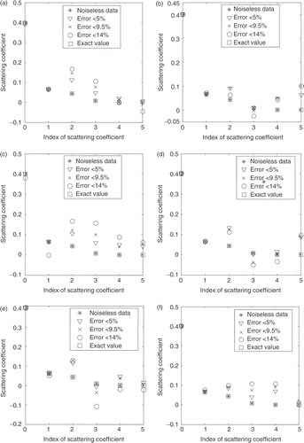
In figures 7 and 8 the estimated values for the scattering coefficients for test cases 5A and 5B, respectively, are shown. These results were obtained for different numbers of grid nodes in the discretization of the angular domain, ranging from N = 16 up to N = 88 for test case 5A, and up to N = 36 for test case 5B. Higher values of N for test case 5B did not provide good estimates.

Figure 7. Estimated values for the scattering coefficients. Test case 5A: (σ_sl = 0.4, 0.06469, 0.04312, 0.008, 1.7778E−006, 0.00 cm⁻¹). L = 0.5 cm; σ_t = 0.5 cm⁻¹. Error in experimental data: * = 0%; ∇ < 5%; × < 9.5%; and O < 14%. (a) N = 16; (b) N = 20; (c) N = 24; (d) N = 28; (e) N = 32; (f) N = 36; (g) N = 40; (h) N = 44; (i) N = 48; (j) N = 52; (k) N = 72; (l) N = 88.

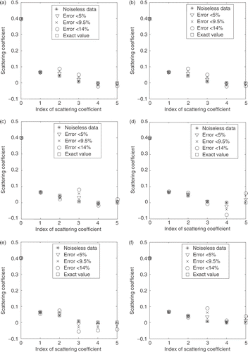
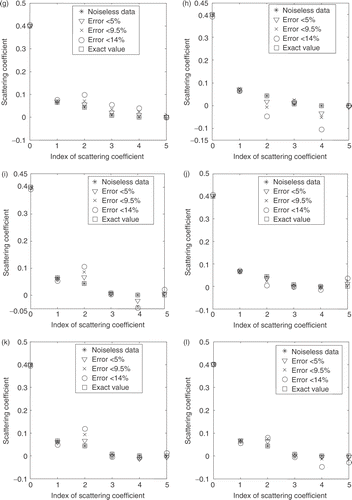
Figure 8. Estimated values for the scattering coefficients. Test case 5B: (σ_sl = 0.4, 0.06469, 0.04312, 0.008, 1.7778E−006, 0.00 cm⁻¹); L = 2.0 cm. σ_t = 0.5 cm⁻¹. Error in experimental data: * = 0%; ∇ < 5%; × < 9.5%; and O < 14%. a) N = 16; (b) N = 20; (c) N = 24; (d) N = 28; (e) N = 32; (f) N = 36.

Similar results were obtained for test cases 6A and 6B using the same levels of noise in the experimental data. The number of grid nodes was varied from N = 16 up to N = 64 for test case 6A, and up to N = 30 for test case 6B.

In tables 7 and 8 the estimated values for the extinction coefficient for test cases 5 and 6, respectively, are presented. In these tables, the lines in bold show the best results obtained in each case.

Table 7. Estimated values for the extinction coefficient () for Test case. (EED = Error in Experimental Data. PRE (%) = Percentage Relative Error = )

N	EED = 0%	PRE (%)	EED < 5%	PRE (%)	EED < 9.5%	PRE(%)	EED < 14%	PRE (%)
(a) Test case 5A (L = 0.5 cm)
16	0.5000	0.0000	0.5072	1.9192	0.5146	2.9129	0.5221	4.4205
20	0.5000	0.0000	0.4891	2.1716	0.4779	4.4241	0.4655	6.9052
24	0.5000	0.0000	0.5012	0.2330	0.5022	0.4327	0.5031	0.6173
28	0.5000	0.0000	0.5069	1.3809	0.5159	3.1729	0.5185	3.6957
32	0.5000	0.0000	0.5018	0.3691	0.5039	0.7788	0.5055	1.0922
36	0.5000	0.0000	0.5001	0.0193	0.5007	0.1420	0.5026	0.5289
40	0.5000	0.0000	0.4955	0.8930	0.4921	1.5873	0.4870	2.6000
44	0.5000	0.0000	0.4996	0.0704	0.5025	0.5081	0.5043	0.8566
48	0.5000	0.0000	0.5007	0.1380	0.5023	0.4644	0.5070	1.4045
52	0.5000	0.0000	0.5016	0.3207	0.5049	0.9826	0.5080	1.5923
72	0.5000	0.0000	0.4931	1.3867	0.4907	1.8643	0.4881	2.3884
88	0.5000	0.0000	0.4955	0.9081	0.4950	0.9901	0.4884	2.3186
(b) Test case 5B (L = 2.0 cm)
16	0.5000	0.0000	0.4991	0.1846	0.5195	3.9021	0.5555	11.1070
20	0.5000	0.0000	0.4596	8.0889	0.4424	11.5161	0.4292	14.1505
24	0.5000	0.0000	0.4759	4.8149	0.4667	6.6591	0.4665	6.7063
28	0.5000	0.0000	0.5075	1.5019	0.4819	3.6180	0.4581	8.3789
32	0.5000	0.0000	0.4721	5.5889	0.4719	5.6233	0.4934	1.3252
36	0.5000	0.0000	0.4646	7.0750	0.4554	8.9192	0.4505	9.8984

Table 8. Estimated values for the extinction coefficient () for Test case 6. (EED: error in experimental data; PRE (%): percentage relative error = )

N	EED = 0%	PRE (%)	EED < 5%	PRE (%)	EED < 9.5%	PRE (%)	EED < 14%	PRE (%)
(a) Test case 6A (L = 0.5 cm)
16	0.5000	0.0000	0.5134	2.6878	0.5282	5.6339	0.5585	11.7079
20	0.5000	0.0000	0.4905	1.8971	0.4786	4.2752	0.4658	6.8304
24	0.5000	0.0000	0.5044	0.8886	0.5091	1.8223	0.5117	2.3426
28	0.5000	0.0000	0.5184	3.6774	0.5311	6.2249	0.5306	6.1136
32	0.5000	0.0000	0.5015	0.2977	0.4988	0.4021	0.4957	0.8669
36	0.5000	0.0000	0.5022	0.4407	0.5047	0.9314	0.5179	3.5882
40	0.5000	0.0000	0.4933	1.3350	0.4933	2.5011	0.4875	6.0894
44	0.5000	0.0000	0.5002	0.0493	0.5052	1.0371	0.5058	1.1567
48	0.5000	0.0000	0.5020	0.4009	0.5096	1.9117	0.5423	8.4651
52	0.5000	0.0000	0.5041	0.8189	0.5108	2.1564	0.5173	3.1329
56	0.5000	0.0000	0.4981	0.3879	0.4932	1.3667	0.4796	4.0755
64	0.5000	0.0000	0.5014	0.2846	0.4981	0.3720	0.4879	2.4177
(b) Test case 6B (L = 2.0 cm)
16	0.5000	0.0000	0.5015	0.2928	0.5160	3.2099	0.5508	10.1583
20	0.5000	0.0000	0.4741	5.1885	0.4655	6.9073	0.4598	8.0460
24	0.5000	0.0000	0.4781	4.3865	0.4655	6.8998	0.3810	23.8056
28	0.5000	0.0000	0.5055	1.0914	0.5065	1.3099	0.4856	2.8885
30	0.5000	0.0000	0.4943	1.1470	0.5108	2.1570	0.4755	4.8923

From figures 7 and 8, and tables 7 and 8, it is observed that the best results were obtained with N varying between 24 and 44 for all test cases with L = 0.5 cm. This range is lower for the test cases with L = 2 cm. For lower values of N the estimates for the scattering and extinction coefficients become degraded. The algorithm did not converge for higher values of the number of grid nodes.

4.2 Estimation of optical thickness, single-scattering albedo and diffuse reflectivities with the implicit formulation

Here, we are interested in estimating the vector of unknowns given by equation (43) using the implicit formulation in which we seek to minimize the Tikhonov's functional given by equation (50) with the regularization terms constructed with the Bregman distances based on the moments of the q-discrepancy as described in sections 3.2 and 3.3.

As real experimental data was not available, we generated synthetic experimental data by adding noise to the calculated values of the radiation intensity, (83) where r_i represents pseudo-random numbers in the range [−1,1], σ emulates the standard deviation of the measurement errors, and N_d is the total number of experimental data available.

In this work, we have considered a Gauss–Legendre quadrature to replace the integral term in equation (3a), with N = 20 collocation points (figure 2). We consider also that the experimental data is acquired at the same grid points used in the angular domain discretization, and therefore N_d = N = 20. Furthermore, half of the experimental data is acquired at τ = 0, with μ < 0, and half at τ = τ₀, with μ > 0.

In order to demonstrate the efficacy of the use of the Bregman distances as the regularization terms in Tikhonov's functional, we have chosen three sets of exact values and initial guesses for which the algorithm without regularization did not converge. The exact values and the initial estimates for the radiative properties are shown in table 9. Here, we consider that the reference values for the unknowns are equal to the exact values.

Table 9. Exact values and initial guesses for test cases I–III

Test case	Exact parameters	Initial guesses
I	{1.0, 0.5, 0.95, 0.5}	{1.5, 0.95, 0.1, 0.1}
II	{1.0, 0.5, 0.1, 0.95}	{5.0, 0.95, 0.95, 0.1}
III	{0.3, 0.5, 0.1, 0.95}	{1.5, 0.95, 0.95, 0.1}

In tables 10–12, the estimated values for the unknowns are presented, for the test cases I, II and III, respectively, at some specific iterations, using σ = 0.0, 0.0025, and 0.005 which correspond to different levels of error in the experimental data. These estimates were obtained with q = 1.5, m = 1.0, and the regularization parameter α = 0.01.

Table 10. Estimated values for the unknowns at some specific iterations with regularization, q = 1.5, m = 1.0, α = 0.01 for Test case I;

Iteration	τ0	ω	ρ1	ρ2	Objective function (Equation (44))
(a) σ = 0.0 (noiseless data)
0	1.5	0.95	0.1	0.1	2.5830
1	1.2875	7.179E−01	7.645E−01	5.378E−01	7.6250E−02
2	1.0060	5.590E−01	8.655E−01	4.827E−01	1.0267E−02
3	1.0005	5.056E−01	9.399E−01	5.006E−01	7.6526E−05
4	1.0000	5.000E−01	9.498E−01	5.000E−01	1.2180E−08
5	9.999E−01	5.000E−01	9.499E−01	5.000E−01	8.9522E−17
⋮	⋮	⋮	⋮	⋮	⋮
10	9.999E−01	5.000E−01	9.499E−01	4.999E−01	4.7703E−19
⋮	⋮	⋮	⋮	⋮	⋮
15	9.999E−01	5.000E−01	9.499E−01	4.999E−01	7.1133E−20
⋮	⋮	⋮	⋮	⋮	⋮
18	9.999E−01	5.000E−01	9.499E−01	4.999E−01	2.2728E−20
⋮	⋮	⋮	⋮	⋮	⋮
(b) σ = 0.0025 (up to 9% error in experimental data)
0	1.5	0.95	0.1	0.1	2.5752
1	1.2793	7.181E−01	7.632E−01	5.424E−01	5.4247E−01
2	1.0110	5.641E−01	8.673E−01	4.884E−01	7.6346E−02
3	1.0075	5.156E−01	9.403E−01	5.050E−01	9.4615E−03
4	1.0056	5.105E−01	9.489E−01	5.049E−01	1.1951E−04
5	1.0054	5.104E−01	9.490E−01	5.050E−01	6.1676E−05
⋮⋮	⋮	⋮	⋮	⋮	⋮
10	1.0054	5.104E−01	9.490E−01	5.050E−01	6.1740E−05
⋮	⋮	⋮	⋮	⋮	⋮
15	1.0054	5.104E−01	9.490E−01	5.050E−01	6.1740E−05
⋮	⋮	⋮	⋮	⋮	⋮
18	1.0054	5.104E−01	9.490E−01	5.050E−01	6.1740E−05
⋮	⋮	⋮	⋮	⋮	⋮
(c) σ = 0.005 (up to 16% error in experimental data)
0	1.5	0.95	0.1	0.1	2.5732
1	1.2724	7.188E−01	7.688E−01	5.457E−01	7.5056E−02
2	1.0069	5.683E−01	8.741E−01	4.915E−01	9.3795E−03
3	1.0000	5.212E−01	9.449E−01	5.090E−01	5.0508E−04
4	9.979E−01	5.165E−01	9.529E−01	5.092E−01	4.5312E−04
5	9.977E−01	5.164E−01	9.529E−01	5.093E−01	4.5310E−04
⋮	⋮	⋮	⋮	⋮	⋮
10	9.977E−01	5.164E−01	9.529E−01	5.093E−01	4.5310E−04
⋮	⋮	⋮	⋮	⋮	⋮
15	9.977E−01	5.164E−01	9.529E−01	5.093E−01	4.5310E−04
⋮	⋮	⋮	⋮	⋮	⋮
18	9.977E−01	5.164E−01	9.529E−01	5.093E−01	4.5310E−04
⋮	⋮	⋮	⋮	⋮	⋮

Table 11. Estimated values for the unknowns at some specific iterations with regularization, q = 1.5, m = 1.0, α = 0.01 for Test case II;

Iteration	τ0	ω	ρ1	ρ2	Objective function (Equation (44))
(a) σ = 0.0 (noiseless data)
0	5.0	0.95	0.95	0.1	5.7647E−01
1	1.9574	8.619E−01	7.805E−01	7.483E−01	1.7833E−01
2	1.0866	7.775E−01	6.164E−01	9.932E−01	1.4217E−02
3	9.251E−01	5.427E−01	2.532E−01	9.696E−01	1.0304E−03
4	9.995E−01	5.050E−01	1.228E−01	9.528E−01	2.1233E−05
5	9.999E−01	5.001E−01	1.008E−01	9.500E−01	2.3721E−08
⋮	⋮	⋮	⋮	⋮	⋮
10	1.0000	5.000E−01	9.999E−02	9.499E−01	1.5660E−18
⋮	⋮	⋮	⋮	⋮	⋮
15	1.0000	5.000E−01	9.999E−02	9.499E−01	2.6945E−19
⋮	⋮	⋮	⋮	⋮	⋮
18	1.0000	5.000E−01	9.999E−02	9.499E−01	9.3734E−20
⋮	⋮	⋮	⋮	⋮	⋮
(b) σ = 0.0025 (up to 3% error in experimental data)
0	5.0	0.95	0.95	0.1	5.7853E−01
1	1.9570	8.620E−01	7.798E−01	7.491E−01	1.7769E−01
2	1.0871	7.781E−01	6.155E−01	9.930E−01	1.4312E−02
3	9.240E−01	5.456E−01	2.554E−01	9.691E−01	1.2084E−03
4	9.977E−01	5.068E−01	1.247E−01	9.525E−01	1.5867E−04
5	9.982E−01	5.019E−01	1.024E−01	9.496E−01	1.3806E−04
⋮	⋮	⋮	⋮	⋮	⋮
10	9.983E−01	5.017E−01	1.015E−01	9.496E−01	1.3808E−04
⋮	⋮	⋮	⋮	⋮	⋮
15	9.983E−01	5.017E−01	1.015E−01	9.496E−01	1.3808E−04
⋮	⋮	⋮	⋮	⋮	⋮
18	9.983E−01	5.017E−01	1.015E−01	9.496E−01	1.3808E−04
⋮	⋮	⋮	⋮	⋮	⋮
(c) σ = 0.005 (up to 7% error in experimental data)
0	5.0	0.95	0.95	0.1	5.8084E−01
1	1.9574	8.599E−01	7.802E−01	6.956E−01	2.4106E−01
2	1.0855	7.595E−01	5.892E−01	9.807E−01	1.0037E−02
3	9.114E−01	5.297E−01	2.393E−01	9.621E−01	8.9792E−04
4	9.880E−01	4.934E−01	1.067E−01	9.551E−01	3.7918E−04
5	9.889E−01	4.886E−01	8.428E−02	9.538E−01	3.5190E−04
⋮	⋮	⋮	⋮	⋮	⋮
10	9.890E−01	4.884E−01	8.329E−02	9.538E−01	3.5159E−04
⋮	⋮	⋮	⋮	⋮	⋮
15	9.890E−01	4.884E−01	8.329E−02	9.538E−01	3.5159E−04
⋮	⋮	⋮	⋮	⋮	⋮
18	9.890E−01	4.884E−01	8.329E−02	9.538E−01	3.5159E−04
⋮	⋮	⋮	⋮	⋮	⋮

Table 12. Estimated values for the unknowns at some specific iterations with regularization, q = 1.5, m = 1.0, α = 0.01 for Test case III;

Iteration	τ0	ω	ρ1	ρ2	Objective function (Equation (44))
(a) σ = 0.0 (noiseless data)
0	1.5	0.95	0.95	0.1	6.5766
1	7.619E−01	8.381E−01	4.253E−01	4.233E−01	1.9813
2	−9.371E−02	6.296E−01	6.465E−02	1.2013	2.3962
3	1.4720	5.070E−01	−4.532E−01	8.843E−01	2.3986E−01
4	2.607E−01	5.870E−01	5.258E−01	9.852E−01	2.5880E−02
5	3.067E−01	4.957E−01	1.959E−01	9.607E−01	9.5534E−03
⋮	⋮	⋮	⋮	⋮	⋮
10	2.999E−01	5.000E−01	9.999E−02	9.499E−01	3.0206E−18
⋮	⋮	⋮	⋮	⋮	⋮
15	2.999E−01	5.000E−01	9.999E−02	9.499E−01	1.9755E−18
⋮	⋮	⋮	⋮	⋮	⋮
18	2.999E−01	5.000E−01	9.999E−02	9.499E−01	1.4043E−18
⋮	⋮	⋮	⋮	⋮	⋮
(b) σ = 0.0025 (up to 9% error in experimental data)
0	1.5	0.95	0.95	0.1	6.5770
1	7.626E−01	8.379E−001	4.260E−01	4.242E−01	1.9780
2	−9.674E−02	6.286E−01	6.570E−02	1.2022	2.4029
3	1.4712	5.069E−01	−4.516E−01	8.847E−01	2.4315E−01
4	2.601E−01	5.866E−01	5.359E−01	9.865E−01	2.931E−02
5	3.082E−01	4.952E−01	2.016E−01	9.619E−01	1.0928E−02
⋮	⋮	⋮	⋮	⋮	⋮
10	3.001E−01	4.997E−01	1.030E−01	9.507E−01	5.697E−05
⋮	⋮	⋮	⋮	⋮	⋮
15	3.001E−01	4.997E−01	1.030E−01	9.507E−01	5.697E−05
⋮	⋮	⋮	⋮	⋮	⋮
18	3.001E−01	4.997E−01	1.030E−01	9.507E−01	5.697E−05
⋮	⋮	⋮	⋮	⋮	⋮
(c) σ = 0.005 (up to 15% error in experimental data)
0	1.5	0.95	0.95	0.1	6.5753
1	7.713E−01	8.382E−01	4.284E−01	4.300E−01	1.9442
2	−1.084E−01	6.331E−01	8.767E−02	1.2168	2.4197
3	1.495E−01	5.073E−01	−3.890E−01	8.900E−01	2.4538E−01
4	2.632E−01	5.719E−01	4.820E−01	9.811E−01	1.8164E−02
5	3.000E−01	4.834E−01	1.722E−01	9.587E−01	6.0057E−03
⋮	⋮	⋮	⋮	⋮	⋮
10	2.966E−01	4.875E−01	9.353E−02	9.510E−01	3.0591E−04
⋮	⋮	⋮	⋮	⋮	⋮
15	2.966E−01	4.875E−01	9.353E−02	9.510E−01	3.0591E−04
⋮	⋮	⋮	⋮	⋮	⋮
18	2.966E−01	4.875E−01	9.353E−02	9.510E−01	3.0591E−04
⋮	⋮	⋮	⋮	⋮	⋮

In tables 10–12, we observe that the algorithm converged even when poor initial guesses were used. When the estimates fall outside the feasible region they are projected back to this region in which there is a physical meaning.

We have then varied the value of the parameters q, m, and α in the ranges 0 < q ≤ 2.5, 0 ≤ m ≤ 3 and 10⁻⁵ ≤ α ≤ 10⁻¹. From a total of 270 runs performed, we have observed that in most cases convergence was achieved with m = 1.0, α = 0.01 or 0.02, and q varying from 0.0 to 2.5. It seems that higher values for q could also be used.

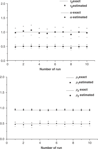
In figures 9–11, the exact values, the estimated values, and the calculated confidence bounds for each of the unknowns are shown. The confidence bounds were calculated with the procedure developed by Gallant 39. Using the notation of Huang and Özisik 40, the standard deviation for the estimates are given by (84) and the confidence bounds for sampling a normal population with 99% confidence are obtained with 41 (85)

Figure 9. Estimates and confidence bounds for test case I using q = 1.5, m = 1.0, α = 0.01, and σ = 0.0025 (up to 9% error in the experimental data).

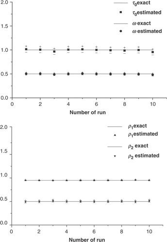
Figure 10. Estimates and confidence bounds for test case II using q = 1.5, m = 1.0, α = 0.01, and σ = 0.0025 (up to 3% error in the experimental data).

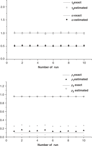
Figure 11. Estimates and confidence bounds for test case III using q = 1.5, m = 1.0, α = 0.01, and σ = 0.0025 (up to 9% error in the experimental data).

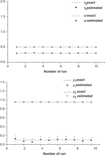
In these figures 10 runs using different sets of random numbers in equation (65), simulating 10 different experiments, are considered. The solid lines represent the exact values of the unknown parameters, and (+) and (−) symbols represent the upper and lower limits of the confidence bounds, respectively.

In figures 9–11, we observe that good estimates are obtained even for experimental data with high level of noise. We observe also that the largest confidence bounds were obtained for the estimates of the parameter ρ₁ in test cases II and III. This is due to the lowest sensitivity to this parameter. This fact was confirmed by a sensitivity analysis.

For all the results presented so far we have considered that the medium is illuminated only from its left side, i.e., τ = 0, and therefore f₁ = 1 and f₂ = 0 in equations (3b) and (3c), respectively. We have also considered only the test cases for which

We now consider a different situation, test case IV, derived from test case I, in which we now have The parameters related to test case IV are listed in table 13.

Table 13. Exact and reference values for test case IV;

Test case	Exact parameters	Initial guesses
IV (derived from test case I)	{1.0, 0.5, 0.95, 0.5}	{1.5, 0.95, 0.1, 0.1}

As shown in table 14, in the first cycle of iterations for test case IV the algorithm converges, but due to the distance of the reference values to the exact parameters it is not able to reach the desired solution. We then restart the algorithm by making After the third cycle, with it reaches the desired solution within a prescribed tolerance. This feedback approach has been used before in a different algorithm developed in 16.

Table 14. Estimated values for the unknowns at specific iterations for test case IV with regularization, q = 1.5, m = 1.0, α = 0.001. σ = 0.005 (up to 16% error in experimental data);

Iteration	τ0	ω	ρ1	ρ2
Cycle 1
0	1.5	0.95	0.1	0.1
1	1.5945	7.259E−1	7.976E−1	3.839E−1
2	1.2444	6.053E−1	8.978E−1	3.920E−1
⋮	⋮	⋮	⋮	⋮
⋮	⋮	⋮	⋮	⋮
20	1.2430	5.775E−1	9.523E−1	4.189E−1
Cycle 2
0	1.2430	5.775E−1	9.523E−1	4.189E−1
1	1.0742	5.255E−1	9.427E−1	4.676E−1
2	1.0616	5.168E−1	9.418E−1	4.705E−1
⋮	⋮	⋮	⋮	⋮
⋮	⋮	⋮	⋮	⋮
20	1.0596	5.160E−1	9.417E−1	4.712E−1
0	1.0596	5.160E−1	9.417E−1	4.712E−1
Cycle 3
1	1.0596	5.305E−1	9.504E−1	4.961E−1
2	1.0557	5.293E−1	9.499E−1	4.974E−1
⋮	⋮	⋮	⋮	⋮
⋮	⋮	⋮	⋮	⋮
20	1.0560	5.294E−1	9.499E−1	4.973E−1

In figure 12, the exact values, the estimated values, and the calculated confidence bounds for each of the unknowns in test case IV, considering 10 runs of the algorithm with different sets of random numbers in equation (65) are shown. These results were obtained at the end of the third cycle of iterations. The solid lines represent the exact values of the unknown parameters, and (+) and (−) symbols represent the upper and lower limits of the confidence bounds, respectively.

Figure 12. Estimates and confidence bounds for test case IV using q = 1.5, m = 1.0, α = 0.01, and σ = 0.005 (up to 16% error in the experimental data).

5. Conclusions

In this work, a brief description was given on some of the explicit and implicit formulations which have been developed and/or implemented by our research group for different inverse problems with applications in engineering, biophysics, and biotechnology.

One new explicit formulation and a family of regularization parameters to be used in implicit formulations are described. From the test case results presented, we observe that the proposed methodologies are robust even in the presence of noisy experimental data and, therefore, deserve further investigation. The results presented are related to one-dimensional problems. In the future, we will pursue the application of the methods developed in multilayer or in multidimensional radiative-transfer problems.

The authors of the present work have been proposing and/or implementing several strategies for the formulation and solution of inverse problems. Regarding parameter estimation inverse problems (finite-dimensional unknowns) there is no single method that presents an overall superior performance. In this instance it seems that hybrid approaches–combining explicit and implicit formulations, or even deterministic and stochastic methods, when inverse problems are implicitly formulated as optimization problems–are the best ones to be attempted. Regarding function estimation inverse problems (infinite-dimensional unknowns) Alifanov's iterative regularization method 42,43 is a very convenient and efficient one due to the simple computational implementation and fast convergence.

Acknowledgements

The authors acknowledge the financial support provided by CNPq–Conselho Nacional de Desenvolvimento Científico e Tecnológico, and FAPERJ–Fundação Carlos Chagas Filho de Amparo à Pesquisa do Estado do Rio de Janeiro.

References

- Sanchez, R, McCormick, NJ, and Yi, HC, 1990. Iterative inverse radiative transfer method to estimate optical thickness and surface albedo, Transport Theory and Statistical Physics 19 (3–5) (1990), pp. 357–385.
- Silva Neto, AJ, 2002. "Explicit and implicit formulations for inverse radiative transfer problems.". In: Proceedings of 5th World Congress on Computational Mechanics, Mini-Symposium MS125–Computational Treatment of Inverse Problems in Mechanics. Austria: Vienna; 2002.
- Alvarez Acevedo, NI, Roberty, NC, and Silva Neto, AJ, 2004. "An explicit formulation for the estimation of the albedo operator in inverse radiative transfer problems.". In: Proceedings of 13th Inverse Problems in Engineering Seminar. USA: Cincinnati; 2004. pp. 1–8.
- Silva Neto, AJ, and Özisik, MN, 1995. An inverse problem of simultaneous estimation of radiation phase function, albedo and optical thickness, Journal of Quantitative Spectroscopy and Radiative Transfer 53 (4) (1995), pp. 397–409.
- Li, HY, and Yang, CY, 1997. A genetic algorithm for inverse radiation problems, International Journal of Heat and Mass Transfer 40 (7) (1997), pp. 1545–1549.
- Silva Neto, AJ, and Soeiro, FJCP, 2002. "Estimation of phase function of anisotropic scattering with a combination of gradient based and stochastic global optimization methods.". In: Proceedings of 5th World Congress on Computational Mechanics. Austria: Vienna; 2002.
- Vasconcellos, JFV, Silva Neto, AJ, Santana, CC, and Soeiro, FJCP, 2002. "Parameter estimation in adsorption columns with a stochastic global optimization method.". In: Proceedings of 4th International Conference on Inverse Problems in Engineering: Theory and Practice. Vol. Vol. II. Brazil: Angra dos Reis; 2002. pp. 227–234.
- Silva Neto, CA, and Silva Neto, AJ, 2003. "Estimation of optical thickness, single scattering albedo and diffuse reflectivities with a minimization algorithm based on an interior points method.". In: Proceedings of 17th International Congress of Mechanical Engineering. Brazil: ABCM. São Paulo; 2003.
- Silva Neto, AJ, and Soeiro, FJCP, 2003. "Solution of implicitly formulated inverse heat transfer problems with hybrid methods.". In: Proceedings of the Mini-Symposium on Inverse Problems form Thermal/Fluids and Solid Mechanics Applications–2nd MIT Conference on Computational Fluid and Solid Mechanics. USA: Cambridge; 2003.
- Soeiro, FJCP, Soares, PO, Campos Velho, HF, and Silva Neto, AJ, 2004. "Using neural networks to obtain initial estimates for the solution of inverse heat transfer problems.". In: Proceedings of Inverse Problems, Design and Optimization Symposium. Brazil: Rio de Janeiro; 2004.
- Soeiro, FJCP, Soares, PO, and Silva Neto, AJ, 2004. "Solution of inverse radiative transfer problems with artificial neural networks and hybrid methods.". In: Proceedings of the 13th Inverse Problems in Engineering Seminar. USA: Cincinnati; 2004. pp. 163–169.
- Cidade, GAG, Anteneodo, C, Roberty, NC, and Silva Neto, AJ, 2000. A generalized approach for Atomic Force Microscopy image restoration with Bregman distances as Tikhonov regularization terms, Inverse Problems in Engineering 8 (2000), pp. 457–472.
- Cidade, GAG, Costa, LT, Weissmüller, G, Silva Neto, AJ, Roberty, NC, Moraes, MB, Prazeres, GMP, Hill, CEM, Ribeiro, SJ, Souza, GGB, Teixeira, LSP, Monçores, MC, and Bisch, PM, 2003. Atomic Force Microscopy as a tool for biomedical and biotechnological studies, Artificial Organs 27 (5) (2003), pp. 447–451.
- Cidade, GAG, Silva Neto, AJ, and Roberty, NC, 2003. Image Restoration with Applications in Biology and Engineering–Inverse Problems in Nanoscience and Nanotechnology. Brazil: SBMAC, São Carlos; 2003, in Portuguese.
- Pinheiro, RPF, Silva Neto, AJ, and Roberty, NC, 2004. "Solution of inverse radiative transfer problems with moments of the q-discrepancy.". In: Proceedings of the 10th Brazilian Congress of Thermal Sciences and Engineering. Brazil: Rio de Janeiro; 2004, in Portuguese.
- Kauati, AT, Silva Neto, AJ, and Roberty, NC, 2001. A source-detector methodology for the construction and solution of the one-dimensional inverse transport equation, Inverse Problems in Engineering 9 (2001), pp. 45–66.
- Kauati, AT, Silva Neto, AJ, and Roberty, NC, 2002. "The source-detector methodology for applications with anisotropic scattering.". In: Proceedings of the 4th International Conference on Inverse Problems in Engineering: Theory and Practice. Vol. Vol. II. Brazil: Angra dos Reis; 2002. pp. 445–452.
- Alvarez Acevedo, NI, Roberty, NC, and Silva Neto, AJ, 2004. A one-dimensional inverse radiative transfer problem with time-varying boundary conditions, Inverse Problems in Science and Engineering 12 (2) (2004), pp. 123–140.
- Alvarez Acevedo, NI, Roberty, NC, and Silva Neto, AJ, 2003. "Estimation of participating media radiative properties with time dependent external illumination.". In: Proceedings of the 18th International Conference on Transport Theory. Brazil: Rio de Janeiro; 2003. pp. 154–161.
- Carita Montero, RF, Roberty, NC, and Silva Neto, AJ, 2004. Reconstruction of a combination of the absorption and scattering coefficients with a discrete ordinates method consistent with the source-detector system, Inverse Problems in Science and Engineering 12 (1) (2004), pp. 81–101.
- Duderstadt, JJ, and Martin, WR, 1979. Transport Theory. New York: Wiley; 1979.
- Özisik, MN, 1973. Radiative Transfer and Interactions with Conduction and Convection. New York: Wiley; 1973.
- Silva Neto, AJ, and McCormick, NJ, 2002. "An explicit formulation based on the moments of the exit radiation intensity for the one-dimensional inverse radiative transfer problem.". In: Proceedings of the 4th International Conference on Inverse Problems in Engineering: Theory and Practice. Vol. Vol. II. Brazil: Angra dos Reis; 2002. pp. 347–354.
- Siewert, CE, 1978. On a possible experiment to evaluate the one-speed or constant cross section model of the neutron transport equation, Journal of Mathematical Physics 19 (1978), pp. 1587–1588.
- Siewert, CE, 1979. On the inverse problem for a three-term phase function, Journal of Quantitative Spectroscopy and Radiative Transfer 22 (1979), pp. 441–446.
- McCormick, NJ, 1979. Transport scattering coefficients from reflection and transmission measurements, Journal of Mathematical Physics 20 (1979), pp. 1504–1507.
- Kaper, HG, Lekkerkerker, CG, and Hejtmanek, J, 1982. Spectral Methods in Linear Transport Theory, in Vol. 5–Operator Theory: Advances and Applications. Basel: Birkhäuser Verlag; 1982.
- Tikhonov, AN, and Arsenin, VY, 1977. Solution of Ill-Posed Problems. New York: Wiley; 1977.
- Calvetti, D, Morigi, S, Reichel, L, and Sgallari, F, 2000. Tikhonov regularization and the L-curve for large discrete ill-posed problems, Journal of Computational and Applied Mathematics 123 (2000), pp. 423–446.
- Muniz, WB, Ramos, FM, and Campos Velho, HF, 2000. Entropy and Tikhonov based regularization techniques applied to the backwards heat equation, Computers & Mathematics with Applications 40 (2000), pp. 1071–1084.
- Roths, T, Marth, M, Weese, J, and Honerkamp, J, 2001. A generalized regularization method for nonlinear ill-posed problems enhanced for nonlinear regularization terms, Computer Physics Communications 139 (2001), pp. 279–296.
- Roberti, D, Campos Velho, HF, and Degrazia, GA, 2002. "Identifying counter-gradient term in convective planetary boundary layer.". In: Proceedings of the 4th International Conference on Inverse Problems in Engineering: Theory and Practice. Vol. Vol. I. Brazil: Angra dos Reis; 2002. pp. 341–348.
- Chandrasekhar, S, 1960. Radiative Transfer. New York: Dover; 1960.
- Bregman, IM, 1967. The relaxation method of finding the common point of convex sets and its application to the solution of problems in convex programming, USSR Computational Mathematics and Mathematical Physics 3 (1967), pp. 200–217.
- Csiszár, I, 1991. Why least squares and maximum entropy? An axiomatic approach to interference for linear inverse problems, Annals of Statistics 19 (4) (1991), pp. 2032–2066.
- Kapur, JN, and Kesavan, HK, 1992. Entropy Optimization Principles with Applications. Boston: Academic Press Inc.; 1992.
- Carita Montero, RF, Roberty, NC, and Silva Neto, AJ, 2001. Absorption coefficient estimation in heterogeneous media using a domain partition consistent with divergent beams, Inverse Problems in Engineering 9 (2001), pp. 587–617.
- Berrocal Tito, MJ, Carvalho, RJ, and Roberty, NC, 2002. "Evaluation of parameters used in a multimedia environmental model–application to Guanabara Bay.". In: Proceedings of the 4th International Conference on Inverse Problems in Engineering: Theory and Practice. Vol. Vol. II. Brazil: Angra dos Reis; 2002. pp. 163–170.
- Gallant, AR, 1987. Nonlinear statistical models. New York: Wiley; 1987.
- Huang, CH, and Özisik, MN, 1990. A direct integration approach for simultaneously estimating spatially varying thermal conductivity and heat capacity, International Journal of Heat and Fluid Flow 11 (1990), pp. 262–268.
- Flach, GP, and Özisik, MN, 1989. Inverse heat conduction problem of simultaneously estimating spatially varying thermal conductivity and heat capacity per unit volume, Numerical Heat Transfer, Part A 16 (1989), pp. 249–266.
- Wang, J-Z, Silva Neto, AJ, Moura Neto, FD, and Su, J, 2002. Function estimation with Alifanov's iterative regularization method in linear and nonlinear heat conduction problems, Applied Mathematical Modelling 26 (11) (2002), pp. 1093–111.
- Su, J, and Silva Neto, AJ, 2001. Heat source estimation with the conjugate gradient method in inverse linear diffusive problems, Journal of Brazilian Society of Mechanical Sciences & Engineering XXIII (3) (2001), pp. 321–334.