Abstract
Inverse analysis is a promising tool of structural diagnosis in the building industry. Though the concept was imported to the field in the early 1980s, the application-oriented developments are still limited. Moreover, the number of investigations that involved experimental work is very small. The current investigation is intended to be an integral ring in the research chain leading to the customization of the inverse analysis in the diagnosis practice of the building industry. The study involves experimental excitation of steel beams with different dynamic characteristics. By utilizing the Kalman filter, as an inverse analysis tool, the experimental response histories were employed, as observations, to identify the simulation parameters of the test beams. The investigation demonstrated that the discrepancies in the stiffness parameters, which are clearly identified, were much smaller than those in the damping ones. This phenomenon is studied and the reason behind it is unveiled. Moreover, the findings of this experimental study highlight the need for further theoretical work to improve the damping identification accuracy.
Nomenclature
| C: | = | Damping coefficient, |
| E: | = | Modulus of elasticity, |
| G: | = | a constant equal to 2√K, |
| K: | = | Stiffness value for SDOF system, |
| KEC: | = | Kinetic energy for continuous system, |
| KEm: | = | Kinetic energy for SDOF system, |
| L: | = | Total beam length, |
| M: | = | Mass of idealized SDOF system, |
| Meq: | = | Lumped mass in a SDOF system equivalent to continuous mass system, |
| M: | = | Total mass of continuous system, |
| m*: | = | Uniform mass per unit length in continuous system, |
| ξ: | = | Damping ratio, and |
| ω: | = | System natural frequency. |
1. Introduction
The inverse analysis concept, originally developed in other fields such as astronomy, acoustics, aerodynamics, and others, was transferred to the field of civil engineering in the early 1980s. When the governing parameters of a given structural system are identified from its response to a certain experimental loading, they can be employed to predict the response of this system to future cases of loading Citation1. An important characteristic of structural and geotechnical civil engineering systems is their continuous geometrical nature. Soils- and super-structures are commonly modelled as continuum with large number of degrees of freedom.
It is evident that obtaining accurate and convergent solutions in the inverse problems becomes harder as the number of degrees of freedom gets larger. Apart from the absolute complexity related to the size of the problem, the fact that the number of observation points and sensors are practically limited causes the ratio, O/F, of the reference observations, O, to the total number of degrees of freedom, F, to become too small to provide adequate information. Such a small ratio results in under-determinacy and ill-posedness for this class of applications.
To overcome this problem, Koh et al. Citation2, utilized the substructuring technique to reduce the number of model degrees of freedom. This approach reduces the size of the problem to only the focal portion of the structure where, for instance, damage detection is sought. Elshazly et al. Citation3,Citation4 introduced and applied a strategy, the VAI method, which identifies a complicated curvilinear stress–strain relationship by successive application of the inverse analysis, using the Kalman filter Citation5, to a simplified linear model.
Lin Citation6 tried to identify soil-modelling parameters from free field response, using down-hole array data. When adopting a three-degree-of-freedom system, he was not able to obtain a convergent solution. It was only possible for him to succeed in his identification bid when he partitioned the problem into three individual SDOF systems.
In this article, the reduction-of-degrees-of-freedom strategy is adopted to identify the dynamic parameters of steel beams with variable concentrated masses at their tips. This modelling is useful for the simulation of many civil engineering structures including elevated tanks, observatories, single storey portal frame construction, and even multistorey tall buildings where the seismic response is governed mainly by the first few modes of vibration. The current study is viewed as an integral addition to the limited number of inverse analysis investigations that applied experimental response data Citation6–8. Moreover, it makes the first address for the phenomenon of the poor convergence of the damping parameters in lightly damped structural systems, and reveals as well as illustrates the cause of this problem. It consequently highlights the need for further theoretical developments to improve the accuracy of identification for this class of application. A research program on these potential improvements has been already launched by the authors.
2. Experimental work
2.1. Test beams
The current study utilizes experimental response records in the identification of dynamic parameters of steel beams. The test beams were fabricated in the laboratory by arranging variable masses at the tip of typical cantilever steel bars, yielding beams with different vibration frequencies and damping coefficients. The cantilever length is 1.10 m and its rectangular cross section is 6 × 60 mm. The total bar mass is therefore 3.055 kg and its experimentally determined Young's Modulus, E, is 2.12 × 10¹¹ N m−2. The tip masses ranged from 0.65 to 119.3% of the total bar mass and were designated accordingly, as S(0.65), S(11.8), S(43.8), S(76.3) and S(119.3).
2.2. Test set-up
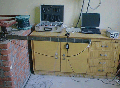
The typical set up for all the test beams is depicted by . The cantilever beam is fixed between two 250 mm long back-to-back angles 70 × 70 × 7 mm each, by means of three 16 mm diameter bolts. The bolts firmly tie the beam to the angles to form a proper fixation. The two angles rest on a 20 mm-thick base plate and linked to it and, further, to the underlying rigid concrete block by means of four welded anchors 19 mm diameter each. During testing, the cantilever beams were excited at their tips to vibrate freely in the horizontal plane.
2.3. Response recording
The test beams S(0.65), S(11.8), S(43.8), S(76.3) and S(119.3) were typically set into free vibration mode, from the static condition, by means of initial displacement of 12 mm. This displacement value, though considerable for the test beams, does not strain them beyond the elastic limit of their material. The acceleration histories were recorded for all beams. In fact, the employed accelerometers represented the tip masses. To simulate larger tip masses, extra accelerometers were attached to the beam tip. These extra accelerometers were also used to double check the quality of the recorded histories.
The length of the recorded acceleration histories was 25 s at a sampling rate of 1000 samples per second, yielding 25,000 observation readings. The linear observation equation incorporated with the coded version of the Kalman filter dictates the use of the velocity and displacement histories as observations rather than the recorded acceleration measurements. The later were therefore integrated so as to obtain the corresponding velocities and displacements, after applying high pass filters to get rid of the low frequency noise components.
2.4. Modal analysis
In order to assess the dynamic characteristics of the test beams, modal analyses were performed using the ME'Scope software Citation9. The advantage of this assessment is to provide check references for the parameters identified using the Kalman filter from the experimental response records. presents the values of the tip masses, the fundamental frequencies, and the damping ratios for all the test beams. The values of the tip masses in the table represent the sum of the bar contribution, as explained in Section 3.2.1, and the masses of the additional accelerations.
Table 1. Dynamic characteristics of test beams.
3. Identification of parameters
3.1. Extended Kalman filter
The extended Kalman filter is an unbiased minimum variance sequential estimation scheme that incorporates the available state information to get a more refined state. The filter structure comprises two basic equations, namely the state and the observation equations. The state equation governs the evolution of the system dynamics with time, and is generally given by
(1)
where X(t) is the state vector at time t, the components of which are the estimated response quantities and parameters at this time. This continuous equation is usually linearized for non-linear problems and takes the form
(2)
When one or some of the response quantities in the state vector are measured and used as input observations to the system, the observation equation can be expressed as
(3)
where Y(t) is the vector of the observed response quantities; H is the observation matrix that relates the observed quantities to the corresponding state vector components; V is a white noise Gaussian sequence vector, which accounts for the contamination in the recorded response.
The filter is then fed with our best estimate at the starting time, X(0), and its covariance matrix P(0). Based on the response observations this initial state of knowledge is continuously updated till reaching the filter's best estimate at the end of the observations. More details about the Kalman filter theory and algorithm can be referred to in Kalman et al. Citation5 and Elshazly et al. Citation3,Citation4.
3.2. Code validation: numerical experiments
3.2.1. Response generation
The Kalman filter scheme Citation5 was coded using the FORTRAN language. In order to ensure the robustness of the developed code of inverse analysis, numerical experiments using synthetic response histories are carried out. In these experiments, known structural parameters are assumed and the corresponding response quantities, including accelerations, velocities, and displacements, are generated using a mathematical model. In the numerical simulation, the cantilever beam is modelled by a single degree of freedom system to simulate the motion of the cantilever tip. Due to the limited space in this article, only one of the performed numerical experiments is presented. In this example, the single degree of freedom stiffness, K, was set at 515.8 N m−1, the system mass, M, at 3.0 kg and the damping ratio, ξ, at 10%. The corresponding damping coefficient, C, is consequently computed using the relation
(4)
A small integration step of 0.001 s was adopted in the generation of the synthetic data.
3.2.2. Parameter identification
A linear observation equation is used in the Kalman filter formulation, and therefore, velocity and displacement histories are employed as observations. A fairly fine sampling rate of 1000 samples per second is adopted in the time discretization in order to improve the convergence of the identified parameters.
Both the observation noise covariance and the error covariance were initially set as diagonal matrices. The diagonal elements of the noise covariance were set at 10−5 for all the observed components of the state vector. There are no concrete guidelines on the choice of the error covariance diagonals for different cases. In all the identification trials, however, a value of 10−5 is adopted for the identified parameters in the state vector. A value of 1.0 is used for the observed elements; that is, for both the displacement and the velocity.
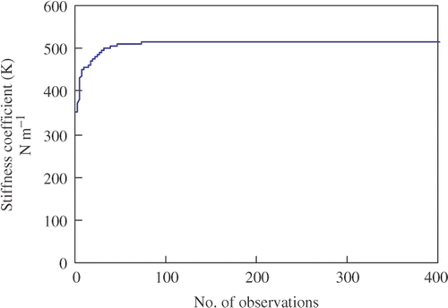
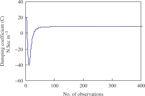
It was found that each of the identified parameters in all the rounds of analyses converged on its own, from its initial estimate to its best estimate. It is, however, found that the identified parameters took about 0.10–0.20 s; that is 100 to 200 observation records, to converge to their best estimates. The convergence curves for the selected example are depicted by Figures and . In all cases, the parameters converged to their stable estimates irrespective of the initial estimates.
The obtained parameters are compared to the original parameters, and the identification errors are computed and presented in . Examination of reveals the fact that both the stiffness and the damping parameters were successfully identified. The error in the damping parameter in this example was 6.41%. In the same case, a minor error of 0.13% was found in the stiffness parameter.
Table 2. Identified damping C and stiffness K for the synthetic beam.
The results of all the numerical experiments, including the example presented above, confirmed the robustness of the Kalman filter scheme and the correctness of the developed inverse analysis codes. The next step will, therefore, be the utilization of the validated code in the identification of the modeling parameters of the test beams from their experimental response records.
3.3. Parameter identification from experimental response records
In the adopted formulation of the inverse problem, the state space vector contained the velocity and the displacement histories as response quantities. This gives rise to a linear observation equation and correspondingly more favorable condition for the convergence of the identified parameters. The parameter part of the state vector contained only the stiffness and the damping parameters, which are set as the identification unknowns. This means that we put more confidence on the usually better-known mass in our bid to obtain knowledge about the uncertain stiffness and damping parameters that are essential to damage detection and structural health monitoring.
3.3.1. Mass contribution
As mentioned above, the reduction of continuous structural systems, with a large number of degrees of freedom, to simpler point mass systems with fewer freedoms, is a useful strategy in inverse analysis applications. It provides simpler state space dimensions and brings around better conditions for convergence by increasing the observations to the freedoms ratio (O/F).
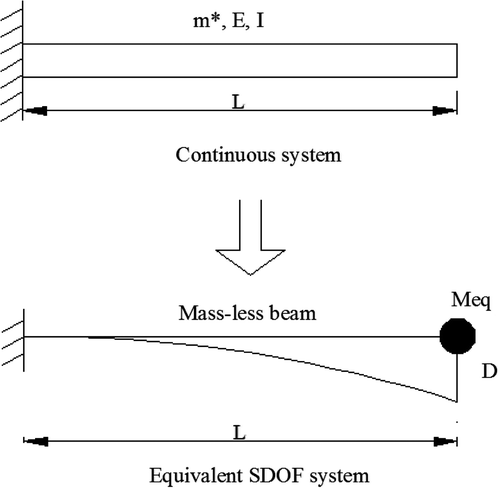
For a cantilever beam excited at the tip, it is evident that its reduction to a SDOF system is a valid simplification, Paz and Leigh Citation10. In this case, the kinetic energy for both the continuous (original) system, KEC, and the point mass (reduced) system, KEm, shall be equal; that is
(5)
For a cantilever excited at its tip in free vibration fashion, the resulting motion shall be dominated by the first mode. Its displacement response, d(x,t) can then be represented by
(6)
where y(x) is the dominant mode shape and ω is the associated frequency. The corresponding velocity, v(x, t), and the maximum kinetic energy, KEC, expressions are
(7)
(8)
where m* is the mass per unit length and L is the cantilever beam length. Let the analytical expression for the first mode, y(x), be assumed as
(9)
where D = y(L) is the tip displacement. By substituting Equation (9) in (8) and integrating, we obtain
(10)
where m is the total beam mass and is equal to m*L. The maximum kinetic energy of the equivalent SDOF system, KEm, at the beam tip is given by
(11)
where Meq is the equivalent (contributed) mass at the cantilever tip. By equating (10) and (11), we obtain the relationship between the equivalent mass, Meq, and the total beam mass, m, as
(12)
It has to be noted that the accuracy of the equivalent mass depends on how perfect the considered modes represent the continuum motion in the respective application ().
3.3.2. Identification of stiffness and damping
The inverse analysis code was verified by a handful of numerical experiments on synthetic data. An example for these experiments was presented in Section 3.2.2. After ensuring the robustness of the Kalman filter code, the response records of the test beams were used to identify their respective dynamic parameters, K and C, based, as illustrated in Section 3.3.1 above, on the assumption that the contributing mass at the cantilever tip is known.
Both the noise covariance and the error covariance were initially set as diagonal matrices. The diagonal elements of the noise covariance were set at 10−5 for the observed components of the state vector. A value of 1.0 is used for the response quantities; that is for both the displacement and the velocity.
For all the identification bids, from the experimental records of the test beams, it was found that the stiffness parameters were successfully identified with minor errors (refer to Tables and ). The damping coefficients, however, contained noticeable discrepancies, and the corresponding errors in the identified damping ratios, as compared to the corresponding modal damping ratios, are substantially large. This can be inferred from . It is obvious that the damping coefficients accuracy is significantly different from that obtained in the numerical experiments, as presented in Section 3.2.2.
Table 3. Identified stiffness K, damping C, and damping ratio ξ.
In order to check the quality of the identified stiffness parameters, each of them was divided by the associated (known) mass, and was compared, in , to the square of the corresponding fundamental frequency, obtained using the modal analysis. The identification error in the square of frequency is computed and presented in the same table. The small values of the computed errors confirm the assumption that the first mode dominates the response and that the stiffness/frequency values were identified with excellent accuracy. It also implies that the adopted SDOF model, in addition to being effective in the inverse analysis convergence, has succeeded to accurately simulate the motions of the test beams.
Table 4. Error in frequency from identified K.
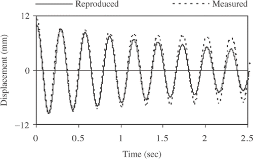
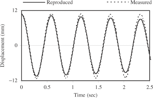
The same conclusion can be reached by the graphical representation of the system response. The measured acceleration and the calculated velocity and displacement histories are compared to those reproduced by incorporating the identified parameters into a SDOF model. Figures and depict examples for the contrast between the measured and the reproduced displacement histories for beams S(11.8) and S(119.3).
The examination of the two figures reveals the fact that the period of oscillation of both the true system and the identified model are almost identical. It is obvious, however, in the two figures that the response of the SDOF system, incorporated with the identified parameters, damps, as previously indicated, faster than the measured beam response. It is also apparent, from the comparison between the fourth cycle of response in the two cases, that the error in damping is smaller in the case of beam S(11.8).
4. Discussion
One can hardly attribute the poor accuracy of the identified damping coefficients to poor functioning of the Kalman filter scheme, or to its coding quality, since numerous experiments have already been successfully performed using the same code, without a single occurrence of odd results. Also, the observation equation in the adopted state space formulation, with observed displacements and velocities, is readily linear and therefore there are no linearization errors.
Table 5. Dependence of accuracy on ξ√Meq.
Despite the fact that the excitation fashion of the test cantilevers gives rise to dominantly first mode response, there are still small contributions of higher modes. These contributions represent small magnitude-high frequency components in the recorded response. They are, therefore, perceived by the Kalman filter as observation noise. This noise, nevertheless, is accounted for in the formulation by setting the noise covariance diagonals at non-zero values.
The fact that the stiffness parameter and consequently the system frequency in all rounds of analyses are excellently identified, as apparent from the coincidence of the measured and the reproduced response histories on the x-axis in Figures and , suggests that the noise level in the response records are too small to be responsible for the poor identification of the damping coefficients. Moreover, the smoothness of the recorded response, as appears in Figures and , tends to support the same argument.
It was also noted that the % error of the damping coefficient in the numerical experiment of Section 3.2.2, despite being small, is always larger than the % error in the corresponding stiffness coefficient. This typical phenomenon, which was observed in the presented example as well as in other numerical experiments, is not, obviously, due to noises, since the synthetic response data were all noise free. Furthermore, we realized that the error in the damping coefficient in the case of the synthetic data is much smaller than the corresponding errors in the damping coefficients in the case of the experimental records.
It is worth mentioning that the damping ratios for the test beams, as determined by modal analysis using the standard package ME'Scope Citation9, are smaller than the damping ratio adopted in the synthetic response example by one order of magnitude or even more. This suggests that the small values of the damping coefficients may have been responsible for their poor identification quality.
In order to further verify this argument, the variation in the value of the coefficient C in all the analysed cases was evaluated. From Equation (4), and due to the fact that the stiffness is constant for all bars, which are identical in cross section and span, it can be concluded that C is proportional to both the damping ratio and the square root of the contributing mass
(13)
where, G is a constant equal to 2√k. The damping ratios, from modal analysis, of different test beams were multiplied by the square root of their corresponding masses and presented together with the Kalman filter determined damping ratios. It was found that the identification error is inversely proportional to this quantity. In other words, the identification accuracy is found to be better in those cases with larger damping coefficient C, or alternatively larger ξ√Meq, than in the cases with smaller ξ√Meq.
The examination of reveals the error trend. The error is largest when ξ√Meq is smallest, as in the case of beam S(0.65). Contrariwise, the error is smallest when ξ√Meq is largest, as in the case of beam S(11.8). Beams S(43.8), S(76.3), and S(119.3) also follow the same trend, in which the error level was found to be inversely proportional to ξ√Meq. If the damping ratio ξ were constant in all the response records, the damping coefficient accuracy would have systematically increased as the tip mass increases, as would have followed from Equation (13).
In both the structural and geotechnical engineering applications, damping ratios in the order of 2.0–8.0% are not uncommon, depending on the constituting material, the strain level, the ambient conditions and the structural geometry. Nevertheless, the damping ratios for the test beams, as obtained from the modal analyses, were smaller than 0.5%. The fact that the beam material is strained within its elastic limit has contributed to decrease the hysteretic damping. Moreover, the special geometrical features of the test beams, and of the similar elevated structures with concentrated tip masses, are believed to be another essential factor, which decreases the viscous damping.
5. Conclusion
This article provides an integral experience on the application of inverse analysis as a non-destructive diagnosis tool in the building industry. Among few investigations, the current study utilizes experimental response records for the identification of dynamic parameters of steel beams. The test beams were fabricated in the laboratory by arranging variable masses, in the range of 0.65–119.3% of the total bar mass, at the tip of typical cantilever steel bars, yielding beams with different vibration frequencies and damping coefficients. It was also found that the ambient conditions during testing have given rise to variable damping ratios. The test beams were set in free vibration mode by means of initial excitations that keep their material within its elastic limit. The acceleration histories of all beams were recorded and integrated twice to get the corresponding velocity and displacement histories, respectively. The integrated histories were employed, as observations, in the Kalman filter scheme, which was coded using the Fortran language, in order to identify the simulation parameters, C and K, of the test beams. At the beginning, the filter code robustness was verified using several sets of synthetic data. An example for these rounds of validation analysis was presented in the article. The following conclusions were inferred from the investigation:
| 1. | The numerical experiments that employed synthetic response data have demonstrated the robustness of the coded Kalman filter scheme in the identification of both the stiffness and the damping parameters. | ||||
| 2. | It was also evident that cantilever beams with concentrated masses, which are essentially continuous systems, can be identified with simulation parameters of reduced point mass systems, possibly down to a SDOF, without sensible compromise on the accuracy. This strategy reduces the number of degrees of freedom in the system equation of the Kalman filter and provides better conditions for the convergence of the identified parameters. Important applications on this are elevated tanks and observatories with significant top masses, as well as other mechanical systems. | ||||
| 3. | In the identification bids for the five test beams, from the experimental records, the stiffness parameters were precisely identified. This was obviously perceivable from the fact that in all cases the response nodes on the time axis coincided for both the recorded and the reproduced histories. This identification quality, as well as the smoothness of the recorded histories, suggests that the noise to signal ratio be very small. | ||||
| 4. | Contrary to the stiffness parameters, and despite the minor noise content in the experimental response, the damping parameters were not accurately identified. | ||||
| 5. | This phenomenon was analysed for all the test beams in view of their dynamic characteristics, their experimental damping ratios as well as their identification outcome. It was shown that the damping parameter accuracy is proportional to the corresponding damping ratio times the square root of the beam mass. The poor identification accuracy for all the test beams can, therefore, be attributed to their small (light) damping ratios. | ||||
| 6. | The current investigation illustrates this phenomenon, which has not been addressed before, and underlines the need for problem-oriented solutions for such a class of lightly damped structures. | ||||
References
- Elshazly, HA, Hafez, D, and Mosaad, MM, 2007. Settlement of circular foundations on stone columns reinforced ground, J. Ground Improvement 11 (3) (2007), pp. 163–170.
- Koh, CG, See, LM, and Balendra, T, 1991. Estimation of structural parameters in time domain: a substructure approach, Earthquake Eng. Struc. Dyn. 20 (1991), pp. 787–801.
- Elshazly, HA, Hasegawa, T, and Murakami, A, 1997. An engineering identification method for curvilinear hysteretic systems excited by varying amplitude dynamic loading, Inverse Prob. Eng. 4 (1997), pp. 177–208.
- 1997. Response prediction of earth structures to future earthquakes based on nonlinear system identification by the VAI method, Inverse Probl. Eng. 5 (1997), pp. 113–144.
- Kalman, RE, and Bucy, RS, 1961. New results in linear filtering and prediction theory, J. Basic Eng. 83(D) (1961), pp. 95–108.
- Lin, JS, 1995. Extraction of dynamic soil properties using extended Kalman Filter, J. Geotech. Eng. ASCE 120 (12) (1995), pp. 249–263.
- Elshazly, HA, Hafez, D, and Mosaad, M, 2006. Back calculating vibro-installation stresses in stone columns reinforced grounds, J. Ground Improvement 10 (2) (2006), pp. 47–53.
- Udwadai, FE, and Jerath, N, 1980. Time variations of structural properties during strong ground shaking, J. Eng. Mech. ASCE 106 (1980), pp. 111–121.
- 2003. ME'Scope, User manual. Jamestown, California, USA: Vibrant Technology Inc.; 2003.
- Paz, M, and Leigh, W, 2004. Structural Dynamics: Theory and Computation. Springer Science + Business Media Inc.; 2004.
