Dynamic observers based on Green's functions applied to 3D inverse thermal models

Abstract

This work develops a new procedure for the use of dynamic observers in inverse heat conduction problem (IHCP). The dynamic observer state technique, used here, is developed to solve not only a one-dimensional but also a three-dimensional heat transfer problem. The IHCP is represented by a classical inverse definition, that is, an unknown heat flux heat is imposed at a front surface of a sample. The heat flux is then estimated by using the dynamic observer techniques and temperature data from a sensor located at the sample far from the heat source. The novelty is the new procedure to obtain the heat transfer function of the system. In this work, this function is derived using Green's function concept instead of taking Laplace transform of a spatially discretized system, as is usual. This procedure allows a great flexibility to the observer technique and represents an easy way to solve multidimensional heat conduction problem. Tests have shown excellent results.

Keywords:

• inverse problem
• dynamic observers
• heat conduction
• heat flux estimation
• Green's functions

Nomenclature

a, b, c, L	=	plate dimensions, m
k	=	thermal conductivity, W m−2 K−1
q	=	heat flux input, W m−2
T	=	temperature, °C
t	=	time, s
T0	=	initial temperature
x, y, z	=	Cartesian coordinates, m
Y	=	measured temperature, °C
f	=	frequency, Hz
G	=	Green's function, m2K W−1
GH	=	heat conductor transfer function, m2K W−1
GQ	=	signal transfer function, m2K W−1
GN	=	noise transfer function, m2K W−1
X(t)	=	input signal in time domain, W m−2
Y(t)	=	output signal in time domain, °C
X(f)	=	input signal in frequency domain, W m−2

Greek Symbols

α	=	thermal diffusivity, m2 s−1
ρ	=	density, kg m−3
θ	=	temperature difference, °C

1. Introduction

The inverse problem can be found in a large area of science and engineering and can be applied in different ways. The greatest advantage of this technique is the ability to obtain the solution of a physical problem that cannot be solved directly. An inverse problem application can be posed by a thermal problem due to a cutting process. It can be observed, in this case, that direct measurement of temperature by using contact-type sensors at the tool–workpiece interface is very dificult in the region due to the cutting movement and the presence of the chip. The use of inverse heat conduction techniques in this problem represents a good alternative since this technique takes into account temperatures measured from accessible positions such as, for example, in the bottom surface of the tool, opposite to its rake face, etc.

Different techniques can be found in the literature for the solution of inverse heat conduction problem (IHCP). For instance, the mollification method 1, the conjugate gradient technique 2, the sequential function specification 3 or the use of optimization techniques such as genetic algorithms 4, simulated annealing 5 or golden section method 6. Techniques based on filters such as the Kalmn filter 7 or dynamic observers 8 has also been employed for the solution of the IHCP.

In the dynamic observer technique, the IHCP solution algorithms are interpreted as filters passing low-frequency components of the true boundary heat flux signal while rejecting high-frequency components in order to avoid excessive amplification of measurement noise 8. The dynamic observers technique proposed by Blum and Marquardt 8, focused on the one-dimensional linear case, which is extended here to solve an inverse multidimensional heat conduction problem.

In order to deal with multidimensional thermal models, this work proposes an alternative way of obtaining the heat transfer function, G_H. Obtaining this function represents an important role in the observer method, and is crucial to allow that the technique be directly applied to three-dimensional heat conduction problems. In this work, the heat conductor transfer function G_H is obtained by using the Green's function concept instead of taking the Laplace transform of the spatially discretized system. This new procedure allows flexibility and efficiency to solve multidimensional inverse problems.

2. Fundamentals

The inverse problem solution based on dynamic observers can be divided in two distinct steps: (i) the obtaining of the transfer function model G_H; (ii) the obtaining of the heat transfer functions G_Q and G_N and the building algorithm identification. A complete description of this technique can be found in the work of Blum and Marquardt 8.

The procedure to obtain the heat transfer function, G_H described by Blum and Marquardt has the greatest advantage of being easily obtained using a mathematical and signal processing software package such as MATLAB® 9. However, for the multidimensional thermal model this procedure cannot be easily implemented due to the great operational cost.

This section presents both a brief description of the usual procedure and the alternative way to obtain the G_H function. The new procedure is based on Green's function concept and on erghotic process properties.

2.1. Heat transfer function obtained using Blum and Marquardt technique: 1D thermal model

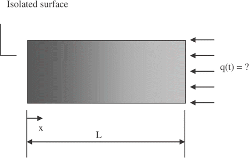
Figure 1 presents a one-dimensional linear heat conduction problem. The system initially at equilibrium temperature T₀ is suddenly exposed to a heat flux at its front surface while the opposite face is kept insulated.

Figure 1. One-dimensional thermal model.

The heat diffusion equation that describes this problem can, then, be given by (1) subjected by the boundary conditions (2) (3) and initial condition (4) where θ = T(x, t) − T₀, α is thermal diffusivity and k is thermal conductivity of the sample in study.

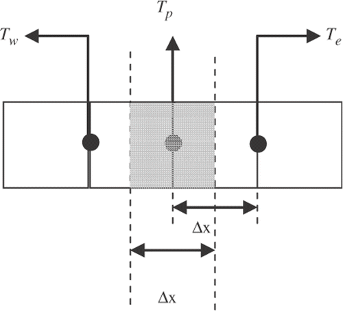
The problem given by Equation (1) can be solved numerically. However, since the heat flux q(t) is an unknown variable, Blum and Marquardt 8 propose to discretize spatially the domain. In which case, by using the discretization scheme shown in Figure 2, Equation (1) assumes the form (5)

Figure 2. Spatially discretized system using finite volume method 10.

Taking the Laplace transform of the spatially discretized system, the transcendental and rational function model in matricial form is (6) Equation (3) can then be solved with symbolic language using the MATLAB® package 9 to obtain (7)

In Equation (4), the coefficients b_i and a_i depend on both the spatial discretization scheme and the discretization order 8. For example, if the number of interior nodes is n_H = 7 the heat transfer function G_H(L, s) calculated at the insulated surface can be given by 11. (8)

Once obtained the function G_H(L, s), the next step is to obtain the estimators G_Q and G_N that are related to G_H through the equation in 8: (9)

In Equation (6), G_Q is referred to as the signal transfer function and G_N is referred to as the noise transfer function. The variable q(s) is the true value of heat flux in Laplace domain and N is random noise due to the temperature measurements. Symbol (⁁) denotes estimated values. The relation between the heat transfer function G_H, G_Q and G_N is described with more details in the next section.

2.2. Obtaining the estimators G_Q and G_N

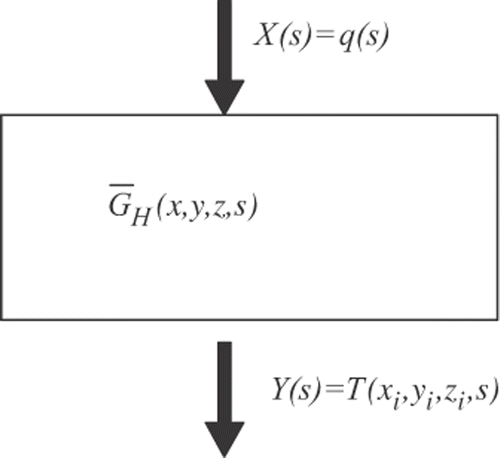
The thermal model described by Equation (1) can be represented by a dynamic system given by a block diagram 8 shown in Figure 3

Figure 3. Frequency-domain block diagram 8.

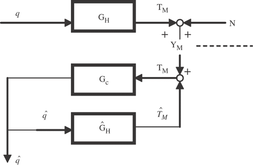
It can be observed from the block diagram that:

(i) The unknown heat flux q(s) is applied to the conductor (reference model), GH, and results in a measurement signal YM corrupted by noise N,

(10)

(ii) The estimate value is computed from the input data YM. Thus, the estimator can be represented in a closed-loop transfer function of the feedback loop as

(11)

Equation (8) characterizes the behaviour of the solution algorithm. The signal and noise transfer function G_Q and G_N can, then, be found by combining Equations (7) and (8) as (12) Thus, from Equation (9) G_N can be written as (13)

It can be observed in Equation (9) that if the algorithm estimates the heat flux correctly, G_Q is equal to unity, G_Q = 1, and the frequency w is within the pass band. In this case, the noise transfer function G_N is equal to the inverse transfer function of the heat conductor (). From Equation (8), the resulting algorithm can be given by (14)

According to Blum and Marquardt 8, the observer is essentially an on-line scheme. In this case, estimation of the heat flux at the current time step is based on current and past temperature measurements only. In this case, any on-line estimator involves a phase shift or lag. To remove this lag, Blum and Marquardt proposes a filtering procedure that can be resumed in the use of two discrete-time difference equations: (15) and (16) In Equations (12) and (13), a_i and b_i are coefficients obtained using Equations (9) and (10). The transfer function G_Q is chosen to have the behaviour of type I Chebychev filter and its frequency response magnitude assume the form (17)

The poles s_cheb,1… are computed using MATLAB package software 9. As mentioned, more details of the observer procedure can be found in ref. 8.

2.3. Heat transfer function, G_H, identification using Green's function: 3D-transient applications

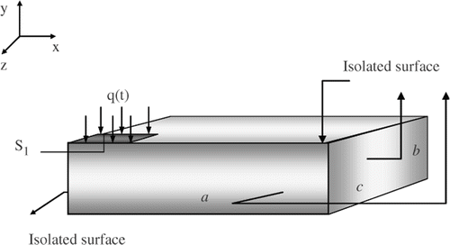
The 3D-transient thermal problem shown in Figure 4 can be described by diffusion equation as (18) In the region R (0 < x < a, 0 < y < b, 0 < z < c) and t > 0, subjected to the boundary condition (19) (20) and initial condition (21) where S is defined by (0 ≤ x ≤ a, 0≤ z ≤ c) and x_H and z_H are the boundary of S₁ where the heat flux is applied.

Figure 4. 3D-transient thermal model.

The solution of Equations (15) can be given in terms of Green's function as in 11. (22) where (23) and G(x, y, z, t − τ) represents the Green's function of the thermal problem given by Equation (15).

The Green's function is available for the homogeneous version associated to the problem defined by Equations (15). Although the analytical Green's function is available and exists 12, it will not be used in this work. On the contrary, the solution of the problem defined by Equation (15) will be performed numerically.

Equation (16) reveals that an equivalent thermal model can be associated with a dynamic model. This means that a response of the input/output system can be associated to Equation (16) in the Laplace domain as the convolution product (24) This dynamic system can be represented as shown in Figure 5.

Figure 5. Dynamic thermal model system.

Equation (16) can also be evaluated in the Laplace domain as a single product 13 (25) where the Laplace transform of a F(t) function is defined by (26)

The heat transfer function can then be obtained through the auxiliary problem, which is an homogenous version of the problem defined by Equation (15) for the same region with a zero initial temperature and unit impulsive source located at the region of the original heating. It means the auxiliary thermal problem can be described as (27) in the region R (0 < x < a, 0 < y < b, 0 < z < c) and t > 0, subjected to the boundary condition (28) (29) and the initial condition (30)

Similarly, the auxiliary thermal problem solution can be derived using Green's function and the convolution properties as (31)

Once the Laplace transform of 1 is (32) then (33)

If the dynamic system is linear, invariant and physically invariable 14, the response function is the same, independently of the pairs input/output and can be obtained by (34) In order to complete the identification, the must be obtained at a specific position r_i = (x_i, y_i, z_i).

A simple and efficient procedure is proposed here to obtain T⁺(r_i, s): if Equation (25) represents a cross correlation function of the two functions of stationary random process s and , then will be independent of the absolute time t and will depend only on the time separation t_a. Figure 6 shows these calculations.

Figure 6. Calculation of cross correlation of G_H.

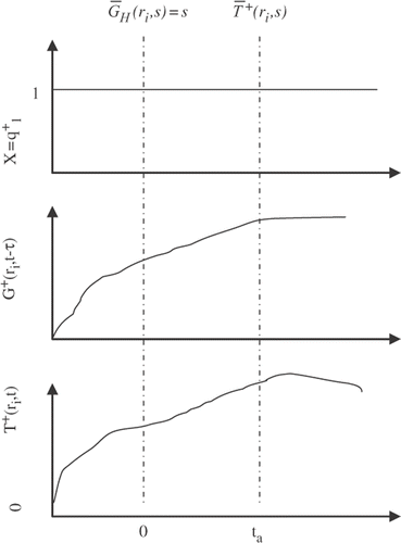
In this case, provided that the function T⁺(r_i, s) can be fitted by a polynomials function in the sampled interval [0, t_a] as (35) where a_i are the polynomial coefficients and taking the Laplace transform of Equation (26), we obtain (36)

Thus, from Equation (25) can be written as (37) (38)

At this point, some observations must be made about Equation (29). It can be observed that from the theory of partial fractions, if is expressible in partial fractions as in Equation (29), its inversion is readily obtained by using the Laplace transform table. Since, Equation (29) does not present any pole for s > 0 then its inversion is stable. This fact guarantees robustness to the inverse algorithm given by Equations (12) and (13). Another advantage of this procedure is the generality of treatment. It means that the same procedure can be used indistinctly by one, two or three-dimensional models, provided the only active boundary condition is the unknown heat source. Once obtained G_H and chebyshev filter (identification of G_Q), the observer technique can be implemented using Equations (12) and (13).

3. Results and discussion

This section presents two cases. First, the new procedure to obtain G_H is compared with the Blum & Marquardt method for one-dimensional transient case. Next, after obtaining G_H. The heat flux estimated is compared with the sequential function estimation method 3 for a three-dimensional transient problem. The first case uses simulated data while both experimental and simulated temperatures are used in the second case.

3.1. Comparison of G_H for the one-dimensional case

The one-dimensional case described in Figure 1 is analysed in this section. Temperature distribution for the direct problem is generated using the solution of Equation (1) considering a known heat flux evolution q(t). Random errors are then added to these temperatures. The temperatures with error are then used in the inverse algorithm to reconstruct the imposed heat flux.

The simulated temperatures are calculated from the following equation (39) where ε_j is a random number. The parameter ε_j assumes values of 0, and within ±0.5°C (1.5% of the maximum temperature) and within ±1.0°C (3.0% of the maximum temperature).

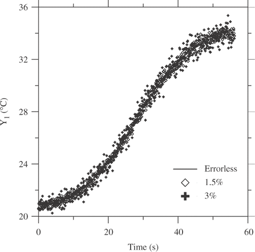
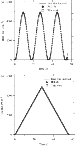
Two test cases simulate a copper sample with a thickness of L = 3 mm, thermal conductivity of k = 401 W mK⁻¹ and thermal diffusivity of α = 117 × 10⁻⁶m² s⁻¹ submitted to two different heat flux types, respectively: (i) a sinusoidal heat flux and; (ii) a triangular heat flux. Figures 7 and 8 present the simulated temperature at the opposite face to the heat fluxes.

Figure 7. Experimental temperatures simulated numerically at x = L, with ε_i = 0.0, within ±0.5°C, within ±1.0°C.: sinusoidal heat flux.

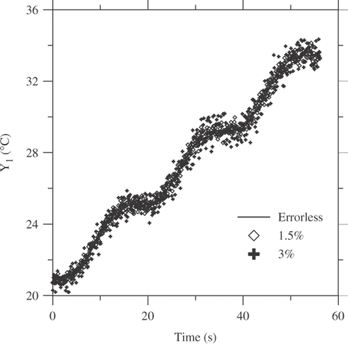
Figure 8. Experimental temperatures simulated numerically at x = L, with ε_i = 0.0, within ±0.5°C, within ±1.0°C.: triangular heat flux.

Figure 9 presents the modulus and phase of G_H obtained using a spatial discretization scheme 8 with 11 volume elements and using the Green's function approach proposed here. It can be observed that modulus and phase values are very close for values of frequencies 100 rad s⁻¹. Therefore, the difference in obtaining the value of G_H just depends on the cut frequency values. For this case, the cut frequency value was w_c = 80 rad s⁻¹ and the heat flux estimated for both methods can be observed in Figure 10 for simulated temperature without noise error for sinusoidal and triangular cases, respectively.

Figure 9. Modulus and phase of heat transfer function, G_H.

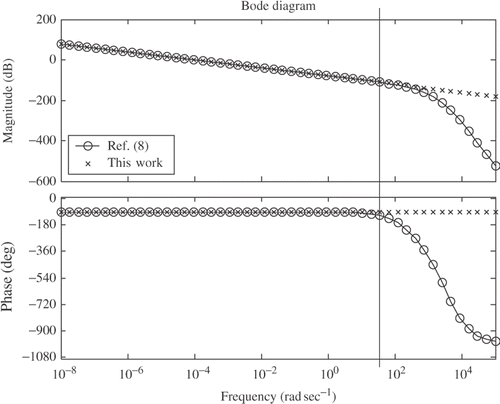
Since the values of w_c = 80 rad s⁻¹ and the heat transfer function value is very close (Figure 9), there is no difference in the estimated heat flux values (Figure 10). The same results can be observed for temperature with noise error. The noise effect will be better explored in the next section for the 3D case.

Figure 10. Heat flux estimation using temperature data without noise error. (a) sinusoidal; (b) triangular.

3.2. Heat flux estimation for a 3D-transient thermal model: simulated and experimental cases

In this section, a 3D-transient application is analysed. Two cases are studied: (i) a simulated case and; (ii) an experimental case.

3.2.1. Simulated case

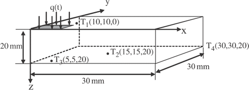
In the simulated case, the same heat flux case studied in the previous section is investigated. Figure 11 presents the simulated temperature sensor locations used to estimate the heat flux.

Figure 11. 3D thermal model test with simulated temperature sensor locations.

Using the same procedure as in the 1D case, the heat flux is estimated using a random noise error addition of the order of 3.0% of the maximum temperature. Figure 12 shows the estimated results.

Figure 12. Heat flux estimation using simulated temperatures, ε_i within ±1.5°C: (a) flux sinusoidal; (b) flux triangular (test 3D).

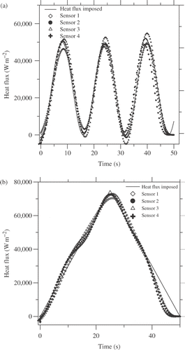
It can be observed that all heat flux estimations are close to the heat flux imposed values although the nearer the sensor to the heat source the better results achieved, as expected.

The good results for all sensors shows the great flexibility of the technique in facing a real problem where the thermocouple positions are limited physically.

3.2.2. Experimental test

An experimental test was carried out in order to analyse the algorithm efficiency. Figure 13 shows the apparatus.

Figure 13. Apparatus experimental scheme.

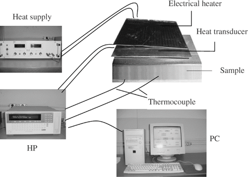
An AISI304 stainless steel sample with a thickness of 47 mm and lateral dimensions of 127 × 127 mm is used in this test. The sample, initially in thermal equilibrium at T₀, is then submitted to a unidirectional and uniform heat flux. The heat flux is supplied by a 318 Ω electrical resistance heater, covered with silicone rubber, with lateral dimensions of 100 × 100 mm and a thickness 0.3 mm. The heat flux are acquired by a transducer with lateral dimensions of 100 × 100 mm, thickness 0.1 mm, and constant time <10 ms. The transducer is based on the thermopile conception of multiple thermoelectric junction (made by electrolytic deposition) on a thin conductor sheet 15. The temperatures are measured using surface thermocouples (type k). The signals of heat flux and temperatures are acquired by a data acquisition system HP Series 75000 with voltmeter E1326B controlled by a personal computer.

In the experiment test, the total number of measurements of each thermocouple was M = 300 with a sampling interval of 0.5 s. The property values used in the thermal model for the AISI304 sample was 14.6 W mK⁻¹ and 3.77 × 10⁻⁰⁶ m² s for thermal conductivity and diffusivity, respectively.

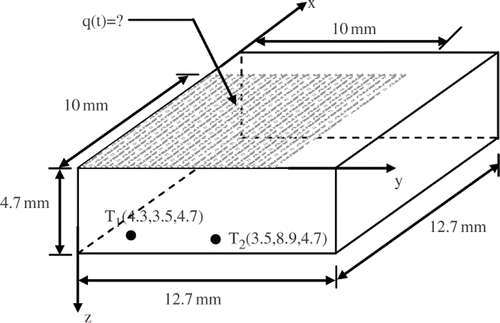
Two thermocouples were brazed on the bottom surface of the sample opposite the surface receiving the heat, at the points T₁(t) and T₂(t) shown in Figure 14.

Figure 14. Thermocouple sensor location and geometric sample description.

Figure 15 shows the experimental temperature evolution Y₁ and Y₂ and Figure 16 shows the measured and estimated heat flux, respectively. A comparison with the sequential fuction especifaction method described by Beck 3 is also shown. The estimation results are very close for both techniques.

Figure 15. Experimental temperature evolution of Y₁(t) and Y₂(t).

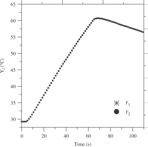
Figure 16. Comparison between the measured and estimated heat flux using Y₁(t).

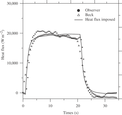
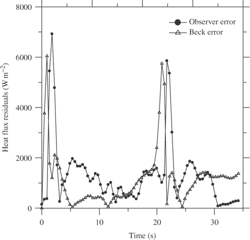
It can be seen that the heat flux is recovered in both heating and cooling regions. However, some oscillations can be observed. This fact is better observed in the residuals calculated from the estimated and experimental heat flux (Figure 17). Figure 17 shows that oscillation reaches the maximum value near the inflexion of the heat flux with values less than 6% for both techniques.

Figure 17. Residuals of heat flux estimated and measured.

The greatest advantage of the dynamic observers technique is the easy and fast numerical implementation for any 1D, 2D or 3D model. The robustness, low computational cost and low-error sensitivity give this procedure great potential in inverse techniques application.

3.3. Non-linear and regularization problem considerations

Despite being a linear operator, Laplace transform can be applied in both linear and non-linear functions. This means that the observer structure shown in Figure 3 can be extended to non-linear problems and, in this case, Equations (12) and (13) must be modified.

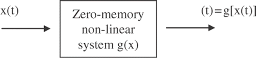
In fact, in order to solve such problems, the non-linearity must be reasonably modelled. In this sense, a non-linear dynamic system can be defined if the temperature dependence of the thermal properties, k(T) and α(T), are well known. One possibility is to define a zero-memory non-linear system which means that an output y(t) at any time t is a single-valued non-linear function of the input x(t) at the same time t 16. Thus, as shown in Figure 18, where g(x) is single-valued non-linear function of x 16.

Figure 18. Zero-memory non-linear system 16.

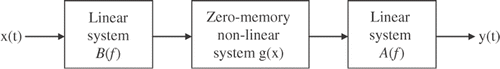
Therefore, an alternative way to solve a non-linear thermal problem is to insert a constant-parameter linear system after and/or before the zero-memory non-linear systems using appropriate frequency response functions A(f) and B(f) as in Figure 19. Effects of g(x) must be taken into account in Equations (12) and (13).

Figure 19. Finite-memory non-linear system with linear systems before and after the zero-memory non-linear system 16.

Although the observer does not use future temperature, the IHCP algorithms are interpreted as filters passing low-frequency components of the true boundary heat flux signal while rejecting high-frequency components in order to avoid excessive amplification of measurement noise. Then the algorithm with the widest ‘pass band’ for a given amplification of measurement noise achieves the best bias-sensitivity trade off. Contrary to the other algorithms, the desired deterministic bias of the observer is imposed directly by specifying the cutoff frequency of the low-pass filter, making tuning both easy and physically meaningful 8.

Blum and Marquardt have compared the observer dynamic method with some regularization techniques (zeroth, first- and second-order) 2 and sequential function specification method (constant heat flux functional form) 3 by determining which algorithm was least sensitive for a given bias. In their work, Blum and Marquardt 8 have demonstrated that the observer has shown lower bias for a given sensitivity or vice versa than Beck's method, regularization approaches, space marching or the Kalman smoother. The order of the observer filter is independent of the sampling interval.

4. Conclusion

The observers method was shown efficient for the IHCP. The presence of random noise in this type of problem is a decisive factor in the choice of technique used since in inverse problems these errors are amplified. The proposal of numerically obtaining the heat function transfer based on Green's functions gives a great flexibility to the technique allowing it to deal with 3D-transient problems both simulated and experimental.

Acknowledgements

We would like to thank Fapemig and CNPq Government Agencies for the financial support of this work.

References

- Murio, DA, 1993. The Molification Method and the Numerical Solution of Ill-posed Problems. New York: John Wiley; 1993.
- Alifanov, OM, 1975. Solution of an inverse problem of heat conduction by iterations methods, Journal of Engineering Physics 10 (1975), p. 471.
- Beck, JV, Blackwell, B, and St. Clair, CR, 1985. Inverse Heat Conduction, Ill-posed Problems. New York: Wiley Interscience Publication; 1985.
- Raudensky, M, Woodbury, KA, Kral, J, and Brezina, T, 1995. Genetic algorithm in solution of inverse heat conduction problems, Numerical Heat Transfer. Part B 28 (1995), p. 293.
- Gonçalves, CV, Vilarinho, LO, Scotti, A, and Guimarães, G, 2006. Estimation of heat source and thermal efficiency in GTAW process by using inverse techniques, Journal of Materials Processing Technology 172 (2006), p. 42.
- Carvalho, SR, Lima e Silva, SMM, Machado, A, and Guimarães, G, 2006. Temperature Determination at the Chip-tool interface using an inverse thermal model considering the tool and tool holder, Journal of Materials Processing Technology 179 (2006), p. 97.
- Tuan, P-C, Ji, C-C, Fong, L-W, and Huang, W-T, 1996. An input estimation approach to on-line two-dimensional inverse heat conduction problems, Numerical Heat Transfer, Part B 29 (1996), p. 345.
- Blum, JW, and Marquardt, W, 1997. An optimal solution to inverse heat conduction problems based on frequency-domain interpretation and observers’, Numerical Heat Transfer, Part B: Fundamentals 32 (1997), p. 453.
- Krauss, T, Shure, L, and Little, J, 1992. MATLAB Signal Processing Toolbox. Natick, MA: The Math-Works Inc.; 1992.
- Patankar, SV, 1980. Numerical Heat Transfer and Fluid Flow. Washington, DC: Hemisphere Publishing Corporation; 1980. p. 197.
- Sousa, PFB, 2006. Development of a technique based on Green's functions and dynamic observers to be applied in inverse problems, Dissertation of Master's degree. Uberlândia, Mg, Brazil: Federal University of Uberlândia; 2006, (in Portuguese).
- Beck, JV, Cole, KD, Haji-Sheik, A, and Litkouhi, B, 1992. Heat Conduction using Green's Function. USA: Hemisphere Publishing Corporation; 1992. p. 523.
- Özisik, MN, 1993. Heat Conduction. New York: John Wiley & Sons; 1993. p. 692.
- Bendat, JS, and Piersol, AG, 1986. Analysis and Measurement Procedures. USA: Wiley-Intersience; 1986. p. 566.
- Guimarães, G, Philippi, PC, and Thery, P, 1995. Use of parameters estimation method in the frequency domain for the simultaneous estimation of thermal diffusivity and conductivity, Review of Scientific Instruments 66 (1995), p. 2582.
- Bendat, JS, 1988. Nonlinear System Techniques and Applications. USA: John Wiley & Sons, INC.; 1988. p. 474.