Aircraft longitudinal stability and control derivatives identification by using life cycle and Levenberg–Marquardt optimization algorithms

Abstract

In this work, two optimization algorithms are investigated to accomplish the parameter identification of the longitudinal motion of a real aircraft by using the output error method. The first algorithm is the nature-inspired algorithm named the life cycle model, which is a composed strategy based on other heuristics such as genetic algorithms and particle swarm optimization. The second one is the gradient-based technique named Levenberg–Marquardt algorithm, which is a variant of the Gauss–Newton method. Flight test data, performed with a training jet aircraft (Xavante AT-26), were used to feed the output error method. In this context, both optimization algorithms were tested, in solo performance and in a cascade-type approach. Results are reported, aiming to illustrate the success of using the proposed methodology.

Keywords:

• system identification
• optimization
• parameter estimation
• evolutionary algorithms

1. Introduction

System identification is a scientific discipline that provides answers to the inverse problem of obtaining a description in some suitable form for a system, given its behaviour as a set of observations 1. Considering that one of the most important phases of the modern design and evaluation process concerns modeling and simulation, the system identification and parameter estimation constitutes a fundamental step to achieve this goal. System identification is a general procedure used to match the observed input–output response of a dynamic system by a proper choice of an input–output model and respective physical parameters. From this point of view, the aircraft system identification or inverse modelling comprises of the proper choice of aerodynamic models, the development of parameter estimation techniques by optimization of the mismatch error between predicted and real aircraft response and the development of proper tools for integration of the equations of motion within the system simulation and correlated activities 2.

The importance of obtaining flight-derived aircraft parameters was recognized early in aircraft evolution. A couple of years after the introduction of the classical stability approach by Bryan 3, Glauert's work in 1919 on the analysis of phugoid motion and that of Norton during 1919–1923 on estimating a number of derivatives mark the beginning of the experimental investigation of dynamic stability from actual flight data 4,5. During the late 1940s and early 1950s, several techniques were introduced, such as steady-state oscillatory excitations by Milliken 6, pulse-input methods incorporating Fourier analysis by Seamans 7, weighted least-squares, and response curve fitting by Shinbrot 8. An excellent account of dynamic stability and control during this early period is found in 9 and a survey of methods for determining stability and control derivatives from dynamic flight measurements in 10.

The techniques of the 1940s to early 1960s were mostly frequency response methods, and were either limited to the estimation of incomplete sets of coefficients, to simple motions, or restricted for other reasons.

Although Shinbrot had introduced the response curve fitting method, which is equivalent to today's output error method, it was at that time found to be impracticable owing to the lack of adequate (digital) computational means. During the early 1960s, analogue matching was a popular technique of updating and validating wind-tunnel predictions of stability derivatives based on flight tests.

The modern era of system identification is marked by the implementation of the maximum-likelihood method on a digital computer by Astrom and Bohlin in 1965, and its application to an industrial plant represented by difference equations 11. The automatic data processing capability provided by digital computers dramatically changed the focus of flight data analysis from frequency-domain methods to time-domain methods. It became possible to obtain a significantly larger number of stability and control derivatives from a single flight test.

Since then, the flight vehicle system identification gradually evolved to a coordinated approach based on flight test techniques, flight test instrumentation and methods of data analysis. All these strongly interdependent topics can be summarized in four important aspects of the art and science of system identification, namely manoeuver, measurements, methods and models. These ‘Quad-M’ requirements must be carefully investigated for each flight vehicle, and are the key to successful flight vehicle system identification 1.

The present work is mainly concerned with the methods aspects and reports the identification of longitudinal stability derivatives from flight test data by using one method in particular, which is the output error method 12,13.

It is well known that the identification by using output error method associated with classical gradient-based optimization methods is a difficult task due to the existence of local minima in the design space. Moreover, such methods require an initial guess to the solution and it is not possible to assure global convergence. These aspects have motivated the authors of this article to explore the performance of a gradient-based, namely the Levenberg–Marquardt method (LM) 13, and a heuristic method, namely the life cycle model (LC) 14. LM is a second-order variant of the Gauss–Newton method and LC is a hybrid approach, based on two heuristic methods, namely genetic algorithms (GA) and particle swarm optimization (PSO) combined in an evolutionary strategy. The individual performance of both algorithms is tested and then a cascade-type scheme is proposed aiming to take advantage of the global search capabilities of LC and the local search capabilities of LM.

An optimization problem is formulated so that the objective function represents the difference between the measured characteristics of the structure and its model counterpart. From a linear state space model for the longitudinal motion of aircraft, a total number of 10 parameters are assumed as being unknown. In this case, the parameters represent the dimensional aerodynamic coefficients of the aircraft.

In order to show the optimization strategy and the approaches, experimental flight test data, performed with a military aircraft (Xavante AT-26), were used in parameter identification of the stability derivatives.

2. Problem formulation

2.1. Aircraft longitudinal model

In this work the inverse problem formulation is applied to the longitudinal equations of movement of the aircraft, in particular, the short period mode, for which the linear state space equations can be written as: (1) and the observation equations are given by: (2)

The previous dynamical equation has 10 unknown parameters that need to be estimated, giving Θ∈ℜ¹⁰: (3)

These parameters Z_α,Z_q,M_α,M_q,Z_δe,M_δe are the stability and control derivatives, which represent the aerodynamic model of the aircraft. The constant parameters b_x1,b_x2,b_y1 and b_y2 comprise measurement biases in the output and input variables, and initial conditions on the state variables.

2.2. Output error method

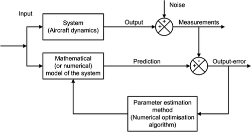
In this section, the parametric identification, in particular the parameter estimation applied to a linear model of the longitudinal motion of an aircraft in space state formulation is presented. The output error method, as shown in Figure 1, is one of the most used estimation methods for aerodynamic parameter estimation from flight test data 15–17. It has several desirable statistical properties, including its applicability to non-linear dynamical systems and the proper accounting of measurements noise 16.

Figure 1. Block diagram of the estimation procedure.

The structure of the model is considered to be known and, in this case, is the one shown in Equations (1) and (2). So, the identification process consists of determining the parameter vector Θ, which gives the best prediction of the output signal y(t), using an optimization criteria. The attainment of an estimate through optimization of a cost function based on the prediction error of the plant requires, usually, the minimization of a non-linear function. Thus, LC, LM or a composition of both is used here to estimate the parameters in the model. Therefore, the cost function to be minimized involves the prediction error: (4) where is the output prediction based on the actual estimate of the parameter vector Θ.

Consider a dynamic system, identifiable, with a defined model M(Θ) and output y. Suppose that p(y | Θ) is the conditional probability Gaussian distribution of the random variable y with dimension m, mean f(Θ), and covariance R, with dimension m × m. p(y | Θ) is known as the likelihood functional. Goodwin and Payne in 12 attribute this name due to the fact that it is a measure of the probability of occurrence of the observation y for a given parameter Θ. Thus, the likelihood functional is: (5)

The maximum likelihood estimate (MLE) is defined as the value of Θ which maximizes this functional, in such a way that the best estimate of Θ is: (6)

The maximization of p(y | Θ) is equivalent to the minimization of the functional J(Θ), which is given by: (7)

Thus, in the optimization process, J(Θ) is equivalent to −ln(p(y | Θ)), except for a constant term.

2.3. Optimization strategies

As can be seen in the general framework illustrated by Figure 1, the output error has no specific requirement about the optimization method. Even though most works in the literature report the use of classical methods, there are no limitations in using other approaches. In this scenario, three optimization strategies, described in Table 1, are explored to solve the identification problem.

Table 1. Optimization strategies used in the output error scheme.

Strategy	Optimization method	Comments
1	Life cycle model	The main explored characteristics are the global search capability and the low level of knowledgement about the search space.
2	Levenberg–Marquart	As a classical method, local search capabilities and small number of function evaluations are the main explored advantages.
3	Life cycle model and Levenberg–Marquart	The result of a first global search performed by LC is used as an initial guess in the LM method. This cascade approach aims to make use of the main advantages of both methods.

3. Life cycle model

3.1. Back to nature

Life cycle model (LC) is a computational tool inspired by the biologic concept of the life cycle. From a biology viewpoint, the term is used here to define the passage through the phases during the life of an individual. Some phases, such as sexual maturity, are one-time events, others, such as mating seasons, are re-occurring. Although it does not happen in every case, the transitions between life cycle phases are started by environmental factors or by the necessity to fit to a new condition 14. The transition process promotes the maturity of an individual and contributes to the adaptation and evolution of its species.

Take the example of a honeybee swarm. Even though 10,000 individuals exist in a colony, there are just three castes of bees:

•	queens, which produce eggs,
•	drones or males, which mate with the queen, and
•	workers, which are all non-reproducing females.

Table 2 shows the life cycles of each bee type in a honeybee colony.

Table 2. Life cycles of bees, measured in days (adapted from 18).

	Queen	Drone	Worker
Egg	3	3	3
Larva	5.5	6.5	6
Cell capped	7.5	10	9
Pupa	8	14.5	12
Period of development	16	24	21
Start of fertility	≈23	≈38	N/A

After this simple example, it is easy to visualize the concept of life cycle.

3.2. Algorithm description

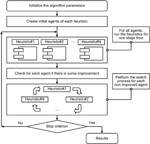
From an implementation point of view, algorithms such as GA and PSO are heuristics search methods of proven efficiency as optimization tools. LC intends to put together the positive characteristics found in each method and creates a self-adaptive optimization approach. Each individual, as a candidate solution, decides based on its success if it would prefer to belong to a population of a GA, or to a swarm of a PSO. This means that different heuristic techniques contribute together to form a robust high-performance optimization tool. The idea is that complex problems can be conveniently considered from the optimization viewpoint. As can be seen, the less successful individuals must change their status in order to improve their fitness. In plain English, the optimization approach does not follow a rigid scheme as proposed in 19, in which various techniques are used sequentially in a cascade-type structure. In other words, it is the mechanism of self-adaptation of the optimization problem that rules the procedure. Figure 2 shows the outline of a basic LC algorithm.

Figure 2. Basic scheme for LC.

Take the example of an LC with just GA and PSO as heuristics. According to Figure 2, the algorithm is initialized with a set of particles of a PSO swarm, which can turn into GA individuals, and then, according to their performance, return to particles again, and so on. An LC individual switches its stage when there is no fitness improvement for more than a previously defined number of iterations. This is a parameter that can be adjusted according to the problem.

3.3. Algorithm parameters

Since the algorithm is composed by various heuristics, it is necessary to set the parameters of every heuristic used in the life cycle. Nevertheless, there is a parameter inherent to the life cycle, namely the number of iterations that represents a stage of the life cycle. The authors, to improve the algorithm performance, have introduced this parameter differently from what is usually done, by simply fixing this number as in 14. This number is called stage interval. At the end of each stage interval, the less successful individuals must change their stage aiming at improving their fitness.

More detailed information about LC can be found in 14,20.

4. Genetic algorithms

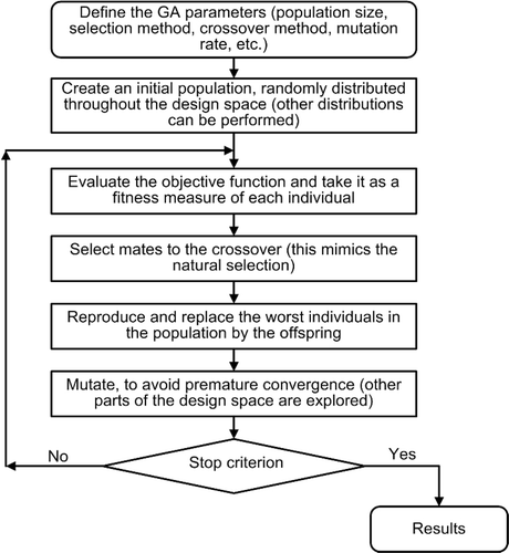
A genetic algorithm is an optimization algorithm based on Darwin's theory of survival and evolution of species. The algorithm starts from a population of random individuals, viewed as candidate solutions to the problem. During the evolutionary process, each individual in the population is evaluated, reflecting its adaptation capability to the environment. Some of the individuals in the population are preserved while others are discarded. This process mimics the natural selection in Darwinism. The remaining group of individuals is paired in order to generate new individuals to replace the worst ones in the population, which are discarded in the selection process. Finally, some of them can be subjected to mutation, and as a consequence, the chromosomes of these individuals are altered. The entire process is repeated until a satisfactory solution is found. The outline of a basic GA is as follows (see Figure 3).

Figure 3. Basic scheme for GA optimization.

Although the initial proposed GA was dedicated to discrete variables, nowadays, improvements are available to deal with discrete and continuous variables, see 21,22 for more details.

5. Particle swarm optimization

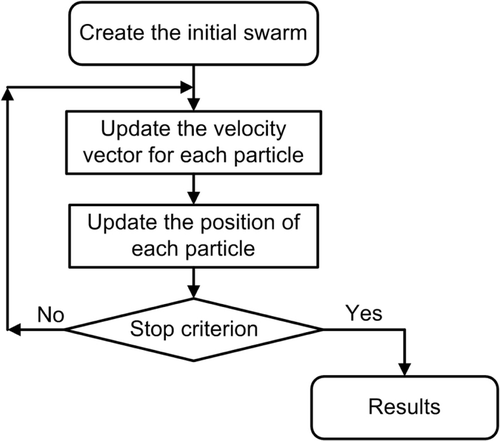
Particle swarm optimization was introduced by Kennedy and Eberhart in 23. The method reflects the social behaviour of some bird species. The main idea of PSO is to reproduce the search procedure used by a swarm of birds when looking for food or a nest. This is achieved by modelling the flying using a velocity vector, somewhat analogous to a search direction. The velocity vector considers a contribution of the current velocity and other two portions referred to the knowledge of the particle itself and of the swarm, respectively, about the search space. In such a way, the velocity vector is used to update the position of each particle in the swarm. The outline of a basic PSO is as follows (see Figure 4):

Figure 4. Basic scheme for PSO optimization.

PSO is comprehensively presented in 23,24.

6. Levenberg–Marquardt optimization method

The Levenberg–Marquardt method is a second-order technique based on the Gauss–Newton method. This method, although complex, is suitable for a quadratic cost function, and is expected to converge quickly. First, we approximate J(Θ) by a parabolic function J_L(Θ) under the condition Θ_L (retaining only the three first Taylor series terms): (8)

The optimization condition is obtained when: (9) Applying Equation (9) to Equation (8): (10) which can be used to find the optimum, Θ*, through the recursion: (11)

The complexity in the calculation of the Hessian matrix, ∇_Θ²J(Θ_i), in Equation (11), is avoided through the Gauss–Newton method, which uses the approximation: (12) where the terms involving the second derivative are discarded and the gradient of the estimated output, , is called sensibility function.

LM is an extension of the Gauss–Newton algorithm 13. The idea is to modify Equation (12) to: (13) where the inversion of the matrix is not performed explicitly, but solving by using singular value decomposition (SVD) we get the following expression: (14)

The addition of the term λI in Equation (14) solves the problem of ill-conditioning of the matrix. The Levenberg–Marquardt algorithm can be interpreted in the following manner: for small values of λ, it behaves like the Gauss–Newton algorithm, while for high values of λ, it behaves like the steepest gradient algorithm.

7. Experimental tests

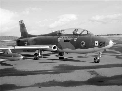
The identification of longitudinal stability derivatives from flight test data was performed by using a set of experimental flight data from a military aircraft. The aircraft used was the Xavante – AT-26 located at the Special Flight Test Group of the CTA (GEEV-CTA), as illustrated in Figure 5. Table 3 reports some geometric and inertial parameters of the aircraft.

Figure 5. Xavante AT-26 training aircraft.

Table 3. Xavante's geometric and inertial parameters.

Symbol	m0	Iy	c	S
Value	4210	6500	1.90	20.62
Unit	kg	kg m^2	m	m^2

The AT-26 was equipped with an instrumentation system in order to collect flight test data for the system identification experiments of this work. Generally, the measurements provided by the flight test instrumentation are introduced to the identification algorithm through the observation equations, as stated in Equation (2).

So, for the present work, the AT-26 flight test instrumentation system provides measurements of the following variables: angle-of-attack, pitch rate and elevator deflection.

In a general manner, the instrumentation system is composed of flight sensors, data acquisition and record unity. The flight sensors that measure the aforementioned variables (angle-of-attack, pitch rate and elevator deflection) have different natures.

The angle-of-attack, being an airflow measurement, requires an air data probe installed in a region of the aircraft in which the minimum disturbance of the inflow air by the aircraft is encountered. This variable is generally measured by vanes and potentiometers. The pitch rate, on the other hand, being an inertial quantity, requires an inertial measurement unit generally installed near the centre-of-gravity of the air vehicle in order to reduce the necessity of some corrections in acceleration measurements. The inertial measurement unit used in the AT-26 flight test instrumentation system is equipped with micro-electro-mechanical gyrometers and accelerometers. The elevator deflection, being a displacement, is generally measured by potentiometers directly installed in the aircraft control surfaces. Table 4 gives some information about the AT-26 measurements of interest for this work.

Table 4. AT-26 measurements characteristics.

Measurement	Acquisition rate (hz)	Acquisition accuracy (%)
Angle-of-attack	32	0.11
Pitch rate	32	0.5
Elevator deflection	16	1.0

For all measurements the existence of systematic errors is assumed, the so-called bias error. As mentioned in section ‘aircraft longitudinal model’, these parameters can also be identified. They take into account some installation and/or sensors inaccuracies during the data acquisition procedure.

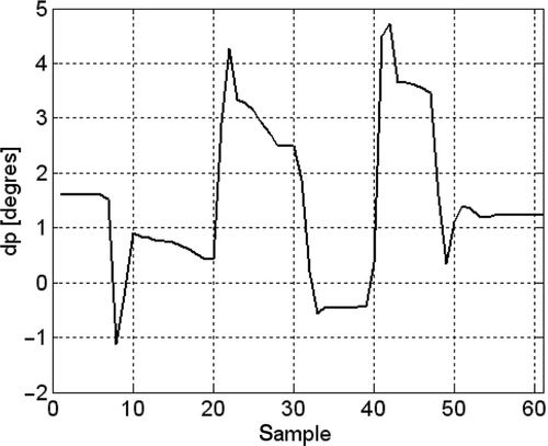
A unique longitudinal flight test manoeuver for collecting the data was used in the present work for identification purposes. The flight test manoeuver was manually applied by the pilot. It was specified in order to excite, mainly, the short period longitudinal dynamic model. Figure 6 shows the elevator deflection measured by the elevator potentiometer during this manoeuver.

Figure 6. Elevator deflection.

8. Results

Table 5 gives the setup for LC used in the identification tests. It is important to point out that the aerodynamic derivatives are a parameter to be estimated as well as the sensors bias errors.

Table 5. Life cycle parameters used in the experimental identification.

	Search space
Parameter	Lower bound	Upper bound
Za	−5	0
Zq	0	5
Ma	−5	0
Mq	−5	0
Zδe	0	5
Mδe	−10	0
bx1	−0.1	0.1
bx2	−0.1	0.1
by1	−0.1	0.1
by2	−0.1	0.1
Population size	50
Number of iterations	200
Stage interval	20

Given the random nature of LC and the dependency of the initial guess of LM, the results obtained using strategy 1 or 2 may vary from one run to another. This way, for the sake a reasonable statistical analysis, each one of the three strategies was repeated 20 times and the best, worst, average, standard deviation, and coefficient of variation of the results from each of the 20 repetitions were recorded. For strategies 1 and 2, LC and LM were set with different and random initial populations and initial guesses, respectively. For strategy 3, the results obtained when running strategy 1 were used as initial guesses for LM. The average indicates the central tendency which the heuristic results tend to. The standard deviation indicates the stability of the optimal solutions, measuring the degree of convergence. In order to express this convergence degree regardless of the magnitude of each of the responses, the coefficient of variation is calculated through the division of the standard variation by the mean value of the optima. It is worth mentioning that the average value for J is the average of values of the functional over the 20 runs; it does not correspond to the value obtained when running the analysis with the average design. Tables 6–8 report a set of identification results obtained following the three different optimization strategies, as presented in Table 1.

Table 6. Identification results for LC (strategy 1).

	Best	Worst	Average	Standard deviation	Coefficient of variation
Za	−1.9439	−1.3795	−2.2321	0.9011	−0.4037
Zq	1.0040	1.1927	0.9939	0.4068	0.4093
Ma	−2.8499	0	−2.0076	1.3095	−0.6523
Mq	−0.8256	−2.9405	−1.4184	0.7578	−0.5343
Zδe	2.7367	2.9498	2.5743	0.9441	0.3667
Mδe	−5.7766	−9.9387	−7.2012	1.8711	−0.2598
bx1	−0.0640	0.0762	−0.0092	0.0559	−6.0659
bx2	0.0988	0.0785	0.0950	0.0079	0.0834
by1	0.0964	0.0659	0.0868	0.0113	0.1298
by2	0.0381	0.0945	0.0621	0.0189	0.3053
J	7.4842 × 10^−9	4.3593 × 10^−8	2.1368 × 10^−8	8.7851 × 10^−9	0.4111

Table 7. Identification results for LM (strategy 2).

	Best	Worst	Average	Standard deviation	Coefficient of Variation
Za	−0.7011	−41.2833^a	−20.8734^a	24.8948	−1.1927
Zq	0.2307	−7.6899^a	6.4499^a	21.3800	3.3148
Ma	−2.3693	−39.5687^a	−2.2620	26.5411	−11.7335
Mq	−1.1758	0.6724^a	1.2852^a	5.3128	4.1339
Zδe	0.3840	11.8288^a	2.8878	30.0194	10.3952
Mδe	−7.1646	8.0484^a	0.0020^a	35.1770	1.8033 × 10^4
bx1	−0.0093	−5.3487^a	−1.2317	3.5939	−2.9179
bx2	0.2037	35.4240^a	1.8770^a	9.2784	4.9432
by1	0.0774	0.0892	2.7547^a	18.7339	6.8007
by2	0.0182	0.0162	2.6264^a	7.1595	2.7260
J	1.1745 × 10^−11	1.1962 × 10^151	7.4764 × 10^149	2.9905 × 10^150	4
^aBoundary violation.

Table 8. Identification results for LC-LM (strategy 3).

	Best	Worst	Average	Standard deviation	Coefficient of Variation
Za	−0.7012	−0.7013	−0.7012	0.0504 × 10^−3	−0.0718 × 10^−3
Zq	0.2308	0.2308	0.2308	0.0235 × 10^−3	0.1019 × 10^−3
Ma	−2.3688	−2.3700	−2.3689	0.5126 × 10^−3	−0.2164 × 10^−3
Mq	−1.1760	−1.1754	−1.1760	0.2443 × 10^−3	−0.2077 × 10^−3
Zδe	0.3841	0.3842	0.3841	0.0795 × 10^−3	0.2069 × 10^−3
Mδe	−7.1653	−7.1634	−7.1652	0.8164 × 10^−3	−0.1139 × 10^−3
bx1	−0.0093	−0.0093	−0.0093	0.0025 × 10^−3	−0.2640 × 10^−3
bx2	0.2037	0.2037	0.2037	0.0108 × 10^−3	0.0530 × 10^−3
by1	0.0774	0.0774	0.0774	0.0037 × 10^−3	0.0472 × 10^−3
by2	0.0182	0.0182	0.0182	0.0016 × 10^−3	0.0854 × 10^−3
J	1.1745 × 10^−11	1.1746 × 10^−11	1.1745 × 10^−11	2.6429 × 10^−16	2.2501 × 10^−5

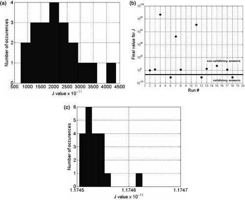
Figure 7 helps the statistical interpretation of the results. Comparing all metrics of the functional J, it is easy to see the advantages of strategy 3. For strategy 1, Table 6 and see Figure 7(a) show that the results found by LC are relatively close to each other, mainly considering the random nature of this algorithm. Strategy 2 was the worst choice by far. From the set of 20 runs, two ended with an indetermination for the value of the functional J, and the other two runs ended with J = +∞ and J = −∞. These facts can have been caused by a numerical ill-conditioning. Consequently, Table 7 was built computing only the remaining 16 runs. It can be seen that for the worst results and for the average of the results as well, there are some boundary violations. At the end, these results were very poor revealing that LM has a strong dependency on the initial guess for finding good results, as illustrated in see Figure 7(b). Finally, Table 8 shows that if properly initialized, LM is capable of ending the local optimization and thus finding solutions extremely close to each other.

Figure 7. J analysis for each strategy. (a) Histogram for LC (strategy 1). (b) Final values for J for LM (strategy 2). (c) Histogram for LC-LM (strategy 3).

Figures 8 and 9 show the performance and convergence of both strategies 1 and 3 for the better and the worse case of each one. They provide a comparison basis to analyse the behaviour of the used techniques.

Figure 8. LC evolution and performance. (a) LC self-adaptation (best case). (b) LC self-adaptation (worst case). (c) LC stage's evolution (best case). (d) LC stage's evolution (worst case). (e) Angle of attack (best case). (f) Angle of attack (worst case). (g) Pitch angular rate (best case). (h) Pitch angular rate (worst case).

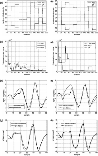
For strategy 1, the evolution and results of the LC can be observed in Figure 8. Figure 8(a) and (b) demonstrate the transitions due to its self-adaptation skills. Figure 8(c) and (d) illustrate which heuristics is conducting the optimization process at a given iteration. Figure 8(e) and (f) give the results for the angle of attack. Finally, Figure 8(g) and (h) show the results for the pitch angular rate. In a certain manner, Figure 8(e)–(h) help to show that even though relatively close, the results found are different one from the other and also they are not good enough to be considered as a final answer for the identification problem.

Figure 9. LC-LM evolution and performance. (a) LM evolution (best case). (b) LM evolution (worst case). (c) Angle of attack (best case). (d) Angle of attack (worst case). (e) Pitch angular rate (best case). (f) Pitch angular rate (worst case).

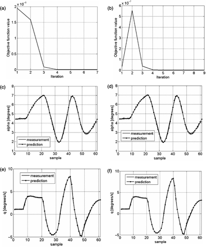
For strategy 3, the evolution and results of the LM can be observed in Figure 9. Figure 9(a) and (b) demonstrate the evolution of the algorithm along the optimization task. Figure 9(c) and (d) illustrate the results for the angle of attack. Finally, Figure 9(e) and (f) give the results for the pitch angular rate. In opposition to what was viewed for strategy 1, Figure 9(c)–(f) clarify that LC is a good way to obtain proper initial designs for LM. In both cases illustrated in Figure 9, the final answers can be considered precise enough for the identification of the problem.

9. Conclusion

This article presented an identification procedure to determine the longitudinal stability and control derivatives of a training jet aircraft. Within the framework of the output error method, the tested optimization algorithms are based on LC and LM methods. In the present contribution, GA and PSO represented the phases of the LC algorithm. The individual performances of both the algorithms were tested and then a cascade-type scheme was proposed, aimed at taking advantage of the global search capabilities of LC and the local search capabilities of LM. Finally, the experimental investigation illustrated the possibility of using the proposed technique in a real world environment. The results are very encouraging in the sense that more complex models, embracing non-linearities, will be analysed in further research.

Acknowledgements

The authors are thankful to the Brazilian Research Agencies, CNPq, and FAPESP, for the PhD and research scholarships granted to some of the authors. Dr Valder Steffen, Jr acknowledges CNPq for the partial financing (Proc. 470346/2006-0) of this research work. Dr Luiz Carlos Sandoval Góes also acknowledges FAPESP (Proc. 01/08753-0) and CNPq (Proc. 312116/2006-3 and 485806/2006-1) for funding part of this research.

References

- Jategaonkar, R, 2006. Flight Vehicle System Identification: A Time Domain Methodology. Reston, Virginia, USA: American Institute of Aeronautics and Astronautics; 2006.
- Jategaonkar, R, Fischenberger, D, and von Gruenhagen, W, 2003. "Aerodynamic modeling and system identification from flight data". In: Recent Application at DLR. In 2nd CTA/DLR Workshop on Data Analysis and Flight Control, São José dos Campos. Brazil. 2003.
- Bryan, GH, 1911. Stability in Aviation. London: McMillan; 1911.
- Glauert, H, 1919. Analysis of phugoids obtained by a recording airspeed indicator (1919), A.R.C. R&M 576.
- Norton, FH, 1923. A study of longitudinal dynamic stability in flight (1923), NACA Report 170.
- Miliken, WF, 1947. Progress in dynamic stability and control research, J. Aeronaut. Sci. 14 (9) (1947), pp. 493–519.
- Seamans, RC, Blasingame, BP, and Clementson, GC, 1950. The pulse method for the determination of aircraft dynamic performance, J. Aeronaut. Sci. 17 (1) (1950), pp. 22–38.
- Shinbrot, M, 1951. A least-squares curve fitting method with applications to the calculation of stability coefficients from transient response data (1951), NACA TN 2341.
- Miliken, WF, 1951. Dynamic stability and control research. Presented at Proceedings of the 3rd Anglo-American Aeronautical Conference.
- Greenberg, H, 1951. A survey of methods for determining stability parameters of an airplane from dynamical flight measurements (1951), NACA TN-2340.
- Astrom, KJ, and Bohlin, T, 1965. "Numerical identification of linear dynamic systems from normal operating records". In: Proceedings of the 2nd IFAC Symposium on Theory of Self-Adaptive Control Systems. England. 1965.
- Goodwin, GC, and Payne, RL, 1977. Dynamic System Identification – Experiment Design and Data Analysis. New York, USA: Academic Press; 1977.
- Nelles, O, 2001. Nonlinear System Identification: from Classical Approaches to Neural Networks and Fuzzy Models. New York: Springer-Verlag; 2001.
- Krink, T, and Løvberg, M, 2002. The lifecycle model: combining particle swarm optimisation, genetic algorithms and Hill-Climbers, 7th International Conference on Parallel Problem Solving from Nature (2002).
- Iliff, KW, 1989. Parameter Estimation for flight vehicles, J. Guidance, Contr. Dyn. 12 (5) (1989), pp. 609–622.
- Ilif, KW, and Taylor, LW, 1972. Determination of stability derivatives from flight data using a Newton–Raphson minimization technique (1972), Technical Report D-6579, NASA.
- Maine, RE, and Iliff, KW, 1985. Identification of dynamic systems, theory and formulation (1985), Technical Report 1138, NASA.
- 2006. Wikipedia, Honeybee life cycle – Wikipedia, the free encyclopedia (2006), [Online; accessed 25 April 2006.].
- Assis, EG, and Steffen, V, 2003. Inverse problem techniques for the identification of rotor-bearing systems, Inverse Probl. Eng. 11 (1) (2003), pp. 39–53.
- Rojas, JE, Viana, FAC, Rade, DA, and Steffen Jr, V, 2004. Identification of external loads in mechanical systems through heuristic-based optimization methods and dynamic responses, Latin Am. J. Solids Struct. 1 (3) (2004), pp. 297–318.
- Haupt, RL, and Haupt, SE, 2004. Pratical Genetic Algorithms. New York: Wiley-Interscience Publication; 2004.
- Michalewicz, Z, and Fogel, DB, 2000. How to Solve it: Modern Heuristics. New York: Springer-Verlag Inc.; 2000.
- Kennedy, J, and Eberhart, RC, 1995. Particle swarm optimization. Perth, Australia: 1995 IEEE International Conference on Neural Networks; 1995. pp. 1942–1948.
- Venter, G, and Sobieszczanski-Sobieski, J, 2002. "Particle swarm optimization". In: 43rd AIAA/ASME/ASCE/AHS/ASC Structures, Structural Dynamics, and Materials Conference. Denver, USA. 2002.