Assessment of dispersion mechanisms in rivers by means of an inverse problem approach

Abstract

In the present work the dispersion mechanisms in rivers are studied. The related direct and inverse problems are formulated and solved. The direct problem is solved by the finite volume method and the inverse problem by the Levenberg–Marquardt method.

Keywords:

• mass transfer
• contaminant transport
• Levenberg–Marquardt method
• dispersion coefficients estimation

1. Introduction

Dynamic models are important tools used to assess water quality in rivers. They can be used to predict the behaviour of contaminant plumes, to define mixing zones of discharges or to estimate the residence/flushing time of contaminants. These models are based on the well-formulated equations from fluid dynamics, their solution yielding the spatial and temporal distribution of the contaminant 1. The equations are grouped into three sub-models. Water levels and velocities are described by the continuity and momentum equations, which define the hydrodynamic model. Mass transport is expressed by the advection–dispersion equation, incorporating velocities calculated by the hydrodynamic model. For non-conservative contaminants further equations are applied, which describe reactions involving the contaminant and all the interactions between the contaminant and other modelled constituents.

For the advection–dispersion equation, the critical parameters are the dispersion coefficients which take into account all spatial water exchange not related to advection. Variations in bed topography, turbulence generated by bed or wind friction, the presence of gradients and the river flow, may all influence the magnitude of the dispersion coefficients 2,3, which may therefore be subjected to significant temporal and spatial variation.

Inverse problem techniques have been used in many problems concerning mass transport, for example, to locate and quantify a pollution source in a channel 4,5, to estimate the parameters of a groundwater contaminant model 6 and to calibrate watershed models 7,8.

Many theoretical approaches have been used to express the dispersion coefficients, taking into account the velocity and tracer fields. In many cases it can also be empirically estimated through comparison of the predicted and observed concentration distribution of a conservative substance 9–11. Although the latter approach may be useful to a particular situation, such as for a particular river, it has a quite limited predictive capability 12.

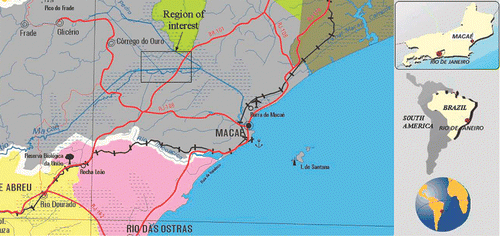
In the present work the dispersion mechanisms in rivers are studied and applied to a particular region of interest, the Macaé river around the effluent discharge from UTE Termomacaé Mario Lago, a Thermoelectric power plant that is run by Petrobras – the Brazilian oil company. Figure 1 illustrates the region represented. The related direct and inverse problems are formulated and solved. The direct problem consists of calculating the contaminant concentration at any position and time, by means of a 2D numerical model (integrated over the depth), considering the known characteristics of the river and contaminant discharge. The inverse problem in which we are interested is the longitudinal and transversal dispersion coefficients estimation with the known concentration measurements taken at given positions and times.

Figure 1. Region of interest location (adapted from Fundação CIDE, http://www.cide.rj.gov.br).

2. Direct problem

A stream of effluent discharged into a river is subjected to two distinct processes. Firstly the waste is mixed across the receiving channel, primarily by turbulence. When the waste is fully mixed across the channel, the process of longitudinal shear flow dispersion together with the turbulence will tend to erase any longitudinal concentration variations.

Adopting a 1D approach for a uniform channel, Elder 13 showed that longitudinal mixing by turbulence eddies is generally unimportant because the shear flow dispersion coefficient caused by the velocity gradient is much bigger than the mixing coefficients caused by turbulence alone. This is particularly valid for the case studied here. The simulated domain was the lower part of Macaé River, basically a straight man-made channel, with regular geometry and a quite low declivity. Further, the simulated scenario was the winter one, when the river discharge and cross-averaged velocities are lower. This particular situation was chosen to represent higher environmental risk for any effluent discharged into the river. During the winter (dry season) the flow velocities are not only low, but also time invariant. This aspect, besides the prevailing regular geometry, makes the assumption of a uniform and non-transient transversal profile of the longitudinal velocity possible.

Although these flow characteristics could be enough to predict a low level of turbulence, this can also be empirically assessed if the river is considered as a uniform open channel. If so, the longitudinal turbulence coefficient (ε) can be expressed as 14 (1) where g (m s⁻²) is the acceleration of gravity, d (m) is the mean depth and S (m m⁻¹) is the declivity. For the prevailing geometry, ε should be around 0.1 m² s⁻¹. Adopting the same simplification, the classical formulation obtained by Elder 14 for the dispersion coefficient would yield a 5.93 higher value.

Considering these aspects, the direct problem here was formulated as: (2) where C is the contaminant concentration, t is time, x is the longitudinal coordinate, y is the transversal coordinate, L and W are the length and the width of the river, respectively, u is the longitudinal velocity, E_L is the longitudinal dispersion coefficient and E_T is the transversal dispersion coefficient.

Using an initial condition, such as (3) a left-side boundary condition, that is, (4) For the right-side boundary condition a fully developed concentration profile was assumed, such hypothesis being checked through a few simulations, when it was adopted a range of values for the parameters. Thus, it was formulated as (5) and at the other boundaries, that is, (6) the concentration of contaminant can be obtained for any location and time of interest C(x, y, t).

Considering the Macaé river flow near the UTE Mario Lago Termomacaé, it is known that the longitudinal velocity is low, therefore can be considered constant, and also considering that the river cross-section area is regular along the river, the longitudinal velocity can be calculated with: (7) where A_c is the river cross-section area and Q is the water volumetric flow rate.

Figure 2 shows a schematic representation of the physical situation considered, showing the contaminant source and the positions where the measurements are performed.

Figure 2. Schematic representation of the river. Notes: S_long.pos = Tracer longitudinal discharging position S_length = Tracer longitudinal discharging length S_trans.pos = Tracer transversal discharging position S_width = Tracer transversal discharging width.

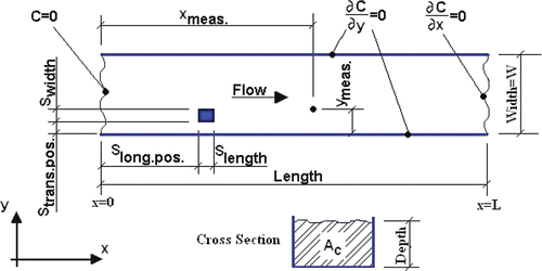
The tracer chosen in this work is common salt (NaCl), but the use of Rhodamine WT could be considered. The latter allows more accurate measurements, but is more expensive. The injection is instantaneous, and its position assumed known.

The direct problem was solved with the well-established implicit upwind finite volume method (FVM). The derivatives necessary to simulate the advection phenomenon were approximated by weighted upstream difference scheme (WUDS) 15.

The spatial discretization generated 4800 cells, being 120 in the longitudinal direction, the first section of 2900 metres was divided in 29 cells of 100 m, the second section with 300 m was divided in 60 cells of 5 m long, the last one with 3100 m was divided in 31 cells of 100 m long. The transversal direction with 42.2 m was divided in 40 cells of 1.055 m.

3. Inverse problem formulation

The inverse problem is implicitly formulated as a finite dimensional optimization problem 16,17 in which one seeks for the minimization of the functional of squared residues (8) where is the vector of measurements, is the vector of calculated values, is the vector of unknown parameters to be determined and the vector of residues corresponds to (9) The inverse problem solution is the vector that minimizes the norm given by Equation (8a), that is (10) Using concentration measurements, C, taken in certain locations along the river, an estimate can be obtained for the vector of unknowns , which is composed by a combination of the following variables: E_L, which represents the longitudinal dispersion coefficient, and E_T, which represents the transversal dispersion coefficient, that is (11) In the absence of real data, the technique is tested using simulated experimental data generated with the direct problem solution obtained with the exact values of E_L and E_T, corrupted by random noise.

4. Design of experiment

Firstly, our objective is to investigate the experiment performed using scaled sensitivity coefficients 18 and the information matrix determinant 19. The objective is to design an optimum experiment to be performed in order to obtain the best possible estimation, i.e. accurate and with a low computational and experimental cost.

The field work has many operational constraints. Sampling must be done in a longitudinal survey, covering as many sites as possible. Further, the costs may impose a limit to the final tracer concentration, which, however, has to be high enough to be detected by the instruments.

Sensitivity analysis plays a major role in several aspects related to the formulation and solution of an inverse problem. Such analysis may be performed with the study of sensitivity coefficients. Here we use the modified, or scaled, sensitivity coefficients (12) where V_i, with i = 1, 2, …, M, is the observable variable, that is, a particular measurement of tracer concentration, M is the total number of measurements, P_j, with j = 1, 2, …, N_p, is a particular unknown of the problem and N_p is the total number of unknowns.

As a general guideline, the sensitivity of the state variable with respect to the parameter we want to estimate must be high enough to allow the estimation of the unknown parameter within reasonable confidence bounds. Moreover, when two or more parameters are simultaneously estimated, their effects on the state variable must be independent (uncorrelated), otherwise these different parameters may affect the state variable in the same way, their influences being difficult to distinguish separately, which leads to poor estimations. Therefore, when graphically represented the sensitivity coefficients should not have the same shape.

In this work we use some techniques related to inverse problems in order to design an experiment to be held at the Macaé River located in the southeast of Brazil, in a region of high environmental interest. As mentioned before, this river receives the effluent of a Thermoelectric power plant which is run by Petrobras. The river characteristics adopted in the simulation are shown in Table 1, following a field survey performed in the region of interest 20.

Table 1. Adopted simulation input data.

Macaé River characteristics	Values
Mean width [m]	42.2
Mean depth [m]	0.71
Volumetric flow rate [m^3 s^−1]	6.0

In order to define the domain, it was necessary to estimate the distance within which a complete mixing across the channel should occur. This measure usually is known as the mixing length. According to Barbosa Junior et al. 10,11, the mixing length can be calculated through an empirical expression, given by where K is a dimensionless parameter, which takes into account the mixing degree and the position and the number of discharges. Adopting K = 0.280, for a mixing degree of the order of 90\%, E_T = 0.56 m² s⁻¹, a value that falls within the range of those found in the literature, and considering the prevailing flow conditions, the mixing length for the simulated discharge should be 177 m. Thus the river section adopted in this study has a length of L = 6.3 km.

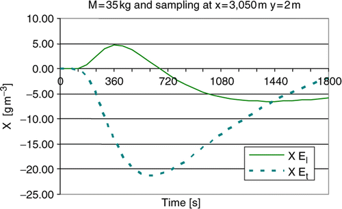
Figure 3 shows the sensitivity coefficients for concentration measurements performed after an instantaneous discharge, at t = 0, of 35 kg of a tracer. The point of tracer discharge considered as x = 3000 m and y = 2 m. The measurements are taken at the position x_meas = 3050 m and y_meas = 2 m. We may be able to estimate simultaneously E_L and E_T since their sensitivities are high and uncorrelated. In order to have a quantitative measure of the correlation between the two curves shown in Figure 3 we are using Pearson's correlation which is often used in hydrological studies concerning water quality of rivers and estuaries, given by (13) For the two curves shown in Figure 3, considering 30 time instants, i.e. M = 30, results R² = 0.0984.

Figure 3. Sensitivity coefficients for sampling at x = 3050 m and y = 2 m.

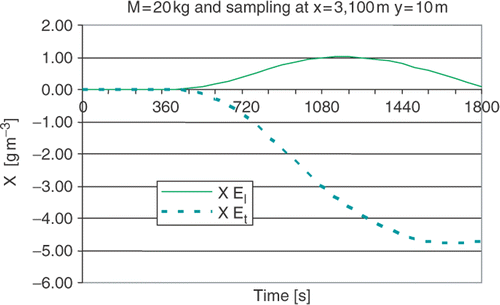
Other possible experiments were also studied, changing the position where the samples are taken, as well as the amount of tracer used. For example, Figure 4 shows the sensitivity coefficients for concentration measurements using 20 kg of tracer and taking samples at the position x_meas = 3100 m and y_meas = 10 m. For this case, using M = 30, Pearson's correlation yields R² = 0.4283, demonstrating that the first experiment would probably lead to better estimates for the vector of unknowns mainly because of two factors: (i) higher tracer amount and (ii) acquisition of experimental data closer to the point of discharge of the tracer.

Figure 4. Sensitivity coefficients for sampling at x_meas = 3100 m and y_meas = 10 m.

Another important tool that can be used to design the experiments is the study of the matrix X^TX, that is, maximizing the determinant of this matrix resulting in higher sensitivity and uncorrelation 19.

The scaled sensivity matrix X is (14) Figure 5 shows the graph of the determinant of matrix X^TX for experiments using different amounts of tracer and with samples being taken at different locations along the river.

Figure 5. Determinant of matrix X^TX for different experiments. [x] = m and [y] = m.

The increase of tracer mass used in the experiment makes the determinant of matrix X^TX higher. However the adopted mass in this study was limited to 35 kg due to practical constraints.

Considering the previous analysis of the sensitivity graphs and the values of the determinant of the matrix X^TX, such experiments were selected whose main control parameters are shown in Table 2.

Table 2. Reference values for the experiment.

Designed experiment	Values
Tracer mass Mtracer [kg]	35.0
Tracer discharge longitudinal position Slong.pos. [m]	3000.0
Tracer discharge transversal position Strans.pos. [m]	2.0
Tracer length Slength [m]	5.0
Tracer width Swidth [m]	1.055
Longitudinal sampling position xmeas [m]	3050.0
Transversal sampling position ymeas [m]	2.0
Initial sampling time t0 [s]	60
Sampling interval Δt [s]	60
Final sampling time tf [s]	1800

5. Inverse problem solution

In this work we used the Levenberg–Marquardt method for the minimization of the cost function given by Equation (8a).

5.1. The Levenberg–Marquardt method (LM)

The Levenberg–Marquardt method 21 is a deterministic local optimizer method based on the gradient. In order to minimize the functional S we first write (15) where J is the Jacobian matrix, whose elements are J_ps = ∂C_calcp/∂P_s, with p = 1, 2, …, N_p, and s = 1, 2, …, M. Observe that the elements of the Jacobian matrix are related to the sensitivity coefficients presented before.

Using a Taylor's expansion and keeping only the terms up to the first order, (16) Introducing the previous expansion in Equation (13) results (17) In the Levenberg–Marquardt method a damping factor λⁿ is added to the diagonal of matrix J^TJ in order to help achieve convergence.

Equation (15) is written in a more convenient form to be used in the iterative procedure, (18) where is the identity matrix and n is the iteration index.

The iterative procedure starts with an estimate for the unknown parameters, , being new estimates obtained with , while the corrections are calculated with Equation (16). This iterative procedure is continued until a convergence criterion such as (19) is satisfied, where ϵ is a small number, e.g. 10⁻⁵.

The elements of the Jacobian matrix, as well as the right-hand-side term of Equation (15), are calculated at each iteration, using the solution of the direct problem with the estimates for the unknowns obtained in the previous iteration.

5.2. Confidence bounds

The confidence bounds for the estimates, , are calculated using the procedure developed by Gallant 22 (20) Assuming a normal distribution on the experimental data error, and 99\% of confidence, the limits of the confidence bounds for the estimates P_j, j = 1, 2, …, N_p, are calculated using 23 (21)

6. Results

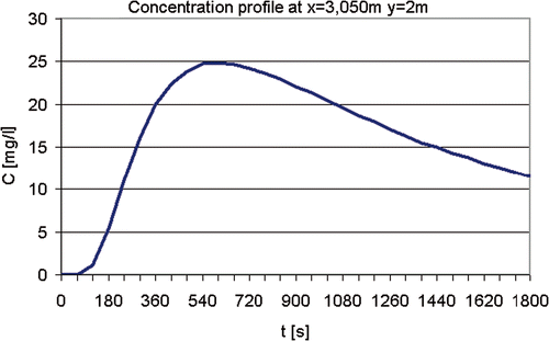
The concentration profile calculated with the exact values at the point of measurement x_meas = 3050 m and y_meas = 2 m is represented in Figure 6.

Figure 6. Concentration measurements taken at x = 3050 m and y = 2 m.

As real experimental data were not available we generated synthetic data using (22) where r_i are random numbers in the range [−1, 1] and σ_e emulates the SD of measurements errors that can be originated from many causes, among them: the amount of tracer material, the river velocity, the sampling position, the measurement techniques and instruments, etc.

Firstly the algorithm was tested using exact data, that is, results generated using the direct problem solution for the designed experiment with σ_e = 0 in Equation (20). The Levenberg–Marquardt method resulted in the original values, numerically validating the inverse problem solution methodology.

Then, simulated experimental data was used, corrupting the direct problem solution for the designed experiment with white Gaussian noise with SD σ = 0.1 g m⁻³, which corresponds to measurement errors of the order of 2\%, being, therefore in the range of expected values due to sampling and analytical errors. The results achieved using the LM for the estimation of E_L and E_T are shown in Figures 7 and 8, respectively. Each figure shows the results for five different runs, considering five different sets of synthetic data, simulating, therefore, five different experiments.

Figure 7. E_L estimates for different runs using the designed experiment. [E_L] = m² s⁻¹.

Figure 8. E_T estimates for different runs using the designed experiment. [E_L] = m² s⁻¹.

For the experiment designed, considering the use of 35 kg of a tracer and measurements to be taken at the position x_meas = 3050 m and y_meas = 2 m, the matrix J^TJ is Observe that in all runs the estimated values are close to the original ones, and within reasonable confidence bounds. The exact values used for the longitudinal and transversal dispersion coefficients in this work are E_L = 5.6 m² s^− 1 and E_T = 0.56 m² s^− 1.

7. Conclusions and future work

The inverse problem approach used for the estimation of the transversal and longitudinal dispersion coefficients achieved good results with both exact and simulated noisy experimental data.

The next step in this research is to test the inverse problem solution using real experimental data and the introduction of improvements in the direct problem solution. Depending on the results obtained with the Levenberg–Marquardt method, it is also in our plans to study the inverse problem solution with artificial neural networks, simulated annealing and hybrid combinations of these methods.

Acknowledgements

The authors acknowledge the financial support provided by CNPq, Conselho Nacional de Desenvolvimento Científico e Tecnológico, CAPES, Coordenação de Aperfeiçoamento de Pessoal de Nivel Superior, and FAPERJ, Fundação Carlos Chagas Filho de Amparo à Pesquisa do Estado do Rio de Janeiro.

References

- Rosman, PC, 1989. "Circulation models in shallow water bodies". In: Vieira da Silva, RC, ed. Numerical Methods in Water Resources. Rio de Janeiro: ABRH; 1989. p. 381, (in Portuguese).
- Harris, J, et al., 1984. A preliminary model of the dispersal and biological effect of toxin in the Tamar estuary, England, Ecol. Model. 22 (1984), pp. 253–284.
- Nielsen, K, Nielsen, LP, and Rasmussen, P, 1995. Estuarine nitrogen retention independently estimated by the denitrification rate and mass balance methods: a study of Norsminde Fjord, Denmark, Mar. Ecol. Prog. Ser. 119 (1995), pp. 275–283.
- Revelli, R, and Ridolfi, L, 2004. Nonlinear convection-dispersion models with a localized pollutant source i: direct initial boundary value problems, Math. Comp. Model. 39 (2004), pp. 1023–1034.
- Revelli, R, and Ridolfi, L, 2005. Nonlinear convection-dispersion models with a localized pollutant source, II – a class of inverse problems, Math. Comp. Model. 42 (2005), pp. 601–612.
- Giacobbo, F, Marseguerra, M, and Zio, E, 2002. Solving the inverse problem of parameter estimation by the genetic algorithms: the case of a groundwater contaminant transport model, Ann. Nucl. Energy 29 (2002), pp. 967–981.
- Bobba, AG, Singh, VP, and Bengtsson, L, 2000. Application of environment models to different hydrological systems, Ecol. Model. 125 (2000), pp. 15–49.
- Dohertyand, J, and Skahill, BE, 2006. An advanced regularization methodology for use in watershed model calibration, J. Hydrol. 327 (2006), pp. 564–577.
- Denves, JA, Barbosa, AR, and da Silva, GQ, 2006. Longitudinal dispersion coefficient quantification model of streams, Eng. San. Ambient. 11 (2006), pp. 269–276, (in Portuguese).
- Barbosa, AR, et al., 2005. Direct methods for the determination of the longitudinal dispersion coefficient in natural bodies of water part 1 – theoretical fundaments, Rev. Esc. Minas. 58 (2005), pp. 27–32, (in Portuguese).
- Barbosa, AR, et al., 2005. Direct methods for the determination of the longitudinal dispersion coefficient in natural bodies of water part 2 – application and comparison of methods, Rev. Esc. Minas. 58 (2005), pp. 139–145, (in Portuguese).
- Rodrigues, PPGW, 2003. "Modelling nitrous oxide production in two contrasting". In: British estuaries: the Forth and The Tyne, PhD Thesis. University of Newcastle upon Tyne; 2003. p. 155.
- Elder, JW, 1959. The dispersion of marked fluid in turbulent shear flow, J. Fluid Mech. 5 (1959), pp. 544–560.
- Fischer, HB, 1959. Mixing in Inland and Coastal Waters. London: Academic Press; 1959. p. 483.
- Maliska, CR, 2004. Computational Heat Transfer, LTC. 2004, LTC-Livros Técnicos e Cientificos, Rio de Janeiro (in Portuguese).
- Neto, AJSilva, 2002. "Explicit and implicit formulations for inverse radiative transfer problems, Proceedings of 5th world congress on computational mechanics". In: Mini-symposium MS125 – Computational Treatment of Inverse Problems in Mechanics. Vienna, Austria. 2002.
- Neto, AJSilva, and Soeiro, FJCP, 2003. "Solution of implicitly formulated inverse heat transfer problems with hybrid methods". In: Mini-Symposium Inverse Problems from Thermal/Fluids and Solid Mechanics Applications – 2nd MIT Conference on Computational Fluid and Solid Mechanics. Cambridge, USA. 2003.
- Dowding, KJ, Blackwell, BF, and Cochran, RJ, 1999. Applications of sensitivity coefficients for heat conduction problems, Numer. Heat Transfer 36 (1999), pp. 33–55.
- Beck, JV, 1988. Combined parameter and function estimation in heat transfer with application to contact conductance, J. Heat Transfer 110 (1988), pp. 1046–1058.
- Amaral, K, 2003. Macaé estuary: modelling as a tool for an integrated management of water resources. Rio de Janeiro, RJ, Brazil: COPPE/UFRJ; 2003. p. 150, M.Sc. Thesis, (in Portuguese).
- Marquardt, DW, 1963. An algorithm for least-squares estimation of nonlinear parameters, J. Soc. Industr. Appl. Math. 11 (1963), pp. 431–441.
- Gallant, AR, 1987. Nonlinear statistical models. New York: Wiley; 1987.
- Flach, GP, and Özisik, MN, 1989. Inverse heat conduction problem of simultaneously estimating spatially varying thermal conductivity and heat capacity per unit volume, Numer. Heat Transfer 16 (1989), pp. 249–266.