Cavity detection in biomechanics by an inverse evolutionary point load BEM technique

Abstract

An efficient solution of the inverse geometric problem for cavity detection using a point load superposition technique in the elastostatics boundary element method (BEM) is presented in this article. A superposition of point load clusters technique is used to simulate the presence of cavities. This technique offers tremendous advantages in reducing the computational time for the elastostatics field solution as no boundary re-discretization is necessary throughout the inverse problem solution process. The inverse solution is achieved in two steps: (1) fixing the location and strengths of the point loads, (2) locating the cavity geometry. For a current estimated point load distribution, a first objective function measures the difference between BEM-computed and measured deformations at selected points. A genetic algorithm is employed to automatically alter the locations and strengths of the point loads to minimize the objective function. Upon convergence, a second objective function is defined to locate the cavity geometry modelled as traction-free surface. Results of cavity detection simulations using numerical experiments and simulated random measurement errors validate the approach in regular and irregular geometrical configurations.

Keywords:

• boundary element method (BEM)
• cavity detection
• genetic algorithm
• elastostatics

1. Introduction

An inverse problem in engineering and science may be defined as one in which a solution is sought for: (a) terms in the governing equation, (b) physical properties, (c) boundary conditions, (d) initial condition(s) or (e) the system geometry, using over-specified conditions. Typically, the over-specified conditions are provided by measuring a field variable at the exposed boundary, as in the case of the inverse geometric problem. However, in some inverse problems, the over-specified condition can be provided by internal measurements of field variable via embedded sensors, see 1–9. In this article, such measurements, along with accompanying noise, are simulated numerically. The purpose of the inverse geometric problem that concerns this study, is to determine the hidden portion of the system geometry by using over-specified boundary conditions on the exposed portion. This problem has gained importance in thermal and solid mechanics applications for nondestructive detection of subsurface cavities Ulrich et al. 8, Kassab et al. 9,10. In thermal applications, the method requires over-specified boundary conditions at the surface, i.e. both temperature and flux must be given, see 7,11,12. In elastostatics applications, the over-specified conditions are provided in terms of surface displacements and tractions. Generally, surface tractions are known boundary conditions, while the surface displacements are experimentally determined by measurements, see Ulrich et al. 8 and Kassab et al. 9.

A variety of numerical methods have been used to solve the inverse geometric problem. This inverse problem has applications in the identification of surfaces flaws and cavities and in shape optimization problems, see 8,9,10,13–16,18. The computational burden is intensive due to the inherent nature of the solution to this inverse problem which requires numerous forward problems to be solved, regardless of whether a numerical or analytical approach is taken to solve the associated direct problem. This is true for generalized cases of irregular geometries when an iterative method is required. Moreover, in the inverse geometric problem, a complete regeneration of the mesh is also necessary as the geometry evolves. Boundary element methods (BEM) lend themselves naturally to the numerical solution of the inverse problem, see 8,9,19–29. This is because the solution algorithms typically involve minimization of residuals, which measure the non-satisfaction of over-specified boundary conditions. Additionally, in the iterative solution of this problem the geometry is continuously updated. This places a premium on a numerical method, which does not require domain discretization, see 30,31.

A method for the efficient solution of the inverse optimization problem of cavity detection using a point load superposition technique in elastostatics BEM is presented in this article. The superposition of point load clusters in the domain is posed as an alternative to satisfy the Cauchy conditions on the surface. The point loads must be located inside the eventual cavity or outside the domain in order to correctly satisfy the governing equation. Using Genetics Algorithms (GA), the point load distribution, strength and location are altered to seek satisfaction of the over-specified boundary displacements. Numerical results of direct 2D problems using the BEM are used as an alternative to validate the approach. Results of cavity detection problems simulated using numerical experiments and added random measurement errors validate the approach in regular and irregular geometrical configurations with single and multiple cavities.

The superposition of point loads as an alternative to simulate the presence of a cavity offers tremendous computational advantages as it allows to pose the inverse problem as a search for the optimal strength and location of such point loads rather than requiring the remeshing of the sought for cavity and thus the recomputation of co-efficients and full solution of algebraic systems at every step of the optimization problem.

2. Elasticity BEM

The solution of the forward elastostatics problem is expressed in terms of displacements which, for an isotropic, homogeneous and linearly elastic medium imposed with an internal volumetric force b_i, is governed by Navier's equation as: (1) Here, is the displacement vector, ν is Poisson's ratio and μ is shear modulus. Introducing the fundamental solution to Navier's equation, a BEM formulation can be derived from the Somigliana identity providing an integral relation between the displacement vector in a point collocation ‘p’ and displacement vectors u_i and traction vectors t_i at the boundary Γ as well as the body forces b_i: (2) Here, Ω is the problem domain, G_ij and H_ij are the displacement and traction fundamental solutions, and is a tensor determined by the boundary geometry at the collocation point p. It is a diagonal matrix with diagonal elements equal to 1 if p is in the interior, 0 if p is at the exterior and (1/2) if p is on smooth boundaries. If p lies on a non-smooth boundary such as a boundary corner, then the unit deflation argument can be used to effectively evaluate the tensor, see 30. Establishing that internal force b_i is formed only by points loads, so that: (3) where NL is the number of points loads, is the intensity of each load and is the Dirac's delta function located in the impact point of each load . Using the properties of the Dirac's delta function, the last integral equation term Equation (2) is reduced to: (4) Employing standard boundary element procedures, the above equation is written in discrete form as: (5) where the matrices [H] and [G], with dimensions N × N, contain the influence co-efficent that relates displacement and traction vectors {u} and {t} on the boundary. The size of N is N = d × NE × NN, where, d is the number of space dimensions (2 or 3), NE is the number of elements and NN is the number of nodes per element. It is worth noting that all effects generated by points loads are located in the vector {q}, therefore, when point loads that are utilized in the inverse geometric problem solution are relocated in the evolving solution, there is no need for boundary re-meshing.

Introducing the boundary condition ū_i and in Equation (5), an algebraic system with the following form is obtained: [A] {x} = {b} + {q}. The vector {x} contains the unknown values of {u} and {t}. This system of equations is solved using a standard method. In this article, quadratic isoparametric discontinuous elements are employed: the geometry and vectors {u} and {t} values are approximated using quadratic shape function locating the displacement and traction nodes within the element boundaries.

3. Cavity simulation

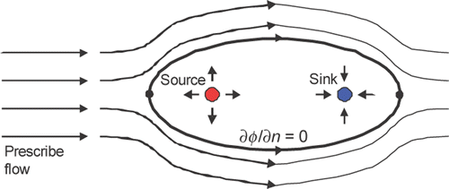
The approach proposed in this article for the modelling of internal cavity(ies) is inspired by potential theory. For example, the superposition of a source and a sink with the same strength located a distance L in a prescribed parallel flow results in iso-flow lines and simulate the presence of a solid surface through the iso-lines containing stagnation points. This null-flow line can be interpreted as the presence of a solid surface or the artificial contour of an elliptical cavity, see Figure 1.

Figure 1. Simulation of elliptical surface with an incoming parallel flow by singularities superposition.

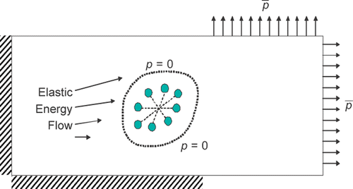
The notion of utilizing point sources and sinks to model cavities has been successfully utilized by Divo et al. 7 in solving the inverse geometric problem by thermal methods. This theory can be applied in elastostatics field where the interpretation is understood as superposition of point loads and the flow is considered to be that of elastic energy. With proper adjustment of the location, number and intensities of these loads, one can generate a surface (or surfaces) that are traction-free and therefore interpreted as a cavity surface(s), this is illustrated in Figure 2, where a cluster of such point loads is shown as an elliptical arrangement with the zero-traction curve drawn around it.

Figure 2. Geometric arrangement of points loads with a non-uniform elastic energy flow.

4. Inverse problem

The numerical inverse process for cavity detection is achieved in 2 steps: (1) fixing the location and strengths of the fictitious point loads and (2) locating the cavity geometry.

For a current estimated point load distribution, a first objective function measures the difference between BEM-computed and measured deformations at the measuring points. Since the governing equation for the elasticity problem is the Navier equation without body forces, the fictitious point loads must be located outside the problem domain, that is, outside the exposed bounding surface or within the subsurface cavities. As such, the first iteration process searches for locations and strengths of the fictitious point loads until a match is found between the tractions and deformations computed by the BEM and those measured on the boundary as additional information or over-specified conditions. This is achieved by the minimization of an objective function: (6) The objective function S₁ quantifies the difference between the deformations u_i obtained by BEM (Equation 5) and measured deformations û_i providing the additional information obtained through experimental measurements on the exposed boundaries, see Divo et al. 7, Ulrich et al. 8, Kassab et al. 9,10. Here, N_m denotes the number of boundary deformation measurements and l = 1, …, L denotes the number of point loads used to simulate the presence of a cavity. It is important to mention that the BEM-computed deformations u_i are a direct function of the parameters that define the strength and location of the point loads.

Once a maximum number of iterations have been performed where the first objective function S₁ does not further change, a second stage of the process is started by defining a second objective function as: (7) The objective function S₂ is minimized to establish the cavity(ies) location(s) indicated as traction-free surface(s). Here, x_i are the points that define the simulated cavity around the cluster of point loads and N_t is the number of points on this curve at which tractions t_i are calculated. A GA is employed to solve both minimization problems and it is parallelized and dynamically balanced.

5. Genetic algorithms optimization

The GA used for this optimization process models the objective function as a haploid with a binary vector to model a single chromosome, see 7,32,33. The length of the vector is dictated by the number of design variables and the required precision of each design variable. Each design variable has to be bounded with a minimum and a maximum value, and in the process the precision of the variable is determined. This procedure allows an easy mapping from real numbers to binary strings and vice versa. This coding process represented by a binary string is one of the distinguishing features of GA and differentiates them from other evolutionary approaches. The haploid GA places all design variables into one binary string, called a chromosome or offspring. The GA optimization process begins by setting a random set of possible solutions. Each individual is defined by a combination of parameters. That is, the strength of the point loads and the location of each point load . An efficient way of parametrizing the location of the point loads to minimize the number of search variables is by requiring them to be arranged in a predefined shape. In this case, a rotated ellipse is employed to arrange the l = 1, …, L point loads. The ellipse is centred at (x_c, y_c) with radii (r_x, r_y) and inclination (θ). All of these search variables are represented as a bit string or chromosome and are bounded by limits that prevent the cluster of point loads to move away from the domain of analysis. However, it is important to mention that should a point load cluster be released to search for a non-existing cavity, the cluster will automatically collapse, vanish, or move outside the geometry during the optimization process.

Since GA are used to maximize and not minimize, a fitness function is formulated as the inverse of the objective function as: (8) This fitness function Z₁ is evaluated for every individual in the current population defining their probability of survival. A series of parameters are initially set in the GA code, and these determine and affect the performance of the genetic optimization process.

The same approach is followed for the second objective function for which a second fitness function is defined as its inverse as: (9) In this case, the search variables x_i that define the shape of the cavity curve around the point load cluster is also parametrized as a rotated ellipse centred at (x_c2, y_c2) with radii (r_x2, r_y2) and inclination (θ₂) in order to minimize the search space dimensions. All of these search variables (x_c2, y_c2, r_x2, r_y2, θ₂) are represented as a bit string or chromosome and are bounded by limits that ensure the line to be outside the point load cluster. This particular parameterization of the cavity shape as a rotated ellipse is by no means general and is simply used as an illustration of the adaptability of the method for the cases studied herein. More general shapes can be conceived where the curve is defined by polar-ray configurations or b-splines to capture more intricate geometries. In addition, the minimization of the second objective function may be easily generalized for cases where the cavity surface is not necessarily traction-free but for instances where an internal pressure or inclusion load is specified. Moreover, the approach lends itself naturally for extensions to three-dimensional problems where the computational advantage of not having to re-mesh during the iteration process is even more pronounced.

6. Examples

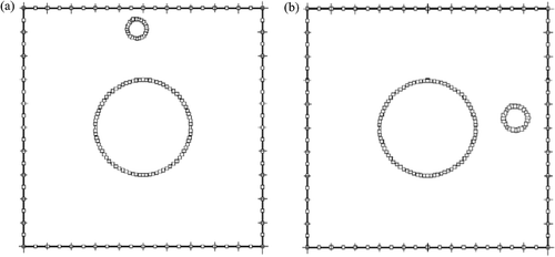
The first example considers a 0.0635 × 0.0635 m² square section with a 0.0254 m diameter-centred hole as shown in Figure 3. The section is made of steel with shear modulus of 60 GPa and a Poisson's ratio of 0.3. Two different cavities are searched in two different runs under the same compression conditions. The first cavity has a diameter of 0.005 m and is located on the top of the section. The second cavity has a diameter of 0.00674 m and is located on the right-hand side of the section. The section is clamped on the left-hand side and the other sides are imposed with 10⁶ Pa uniform compression loads. The two cases are discretized with 80 and 40 quadratic discontinuous isoparametric boundary elements for the square and centred-hole boundaries, respectively, see Figure 4.

Figure 3. Geometry and conditions for square section with centred-circular hole. (a) Top cavity case; (b) Right-hand cavity case.

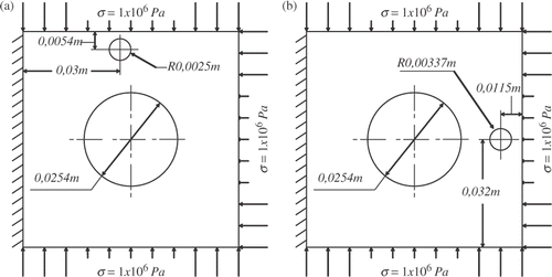
Figure 4. Discretization of square section with centred-hole cases. (a) Top cavity case; (b) Right-hand cavity case.

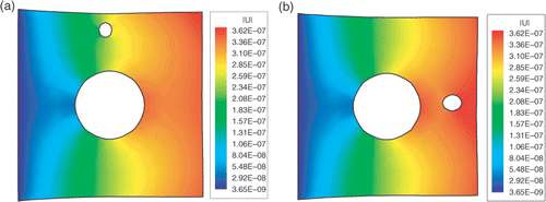
The direct problem is solved for both the top cavity and the right-hand cavity cases. The displacement magnitude contours for both cases are displayed in Figure 5. The BEM-computed displacements on the bottom, right-hand and top boundaries are ladened with a random error of SD ±1 · 10⁻⁸ m to simulate measurement errors, and then used as input for the inverse cavity detection analyses with a number of measurements N_m = 60. A total of L = 4 point loads were employed to simulate the cavity during the first stage of the optimization processes while N_t = 8 points around the defined cluster of point loads were used to calculate the tractions during the second stage of the optimization processes.

Figure 5. Displacement contours of square section with centred-hole cases. (a) Top cavity case; (b) Right-hand cavity case.

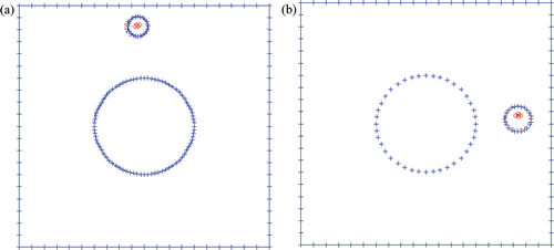
Plots of the objective functions S₁ and S₂ evolution over the optimization process are displayed in Figure 6 for the top cavity case and in Figure 7 for the right-hand cavity case. The prediction of the cavity location (indicated by the dashed line) along with the location of the point loads (indicated by small circles) is displayed for the top cavity and right-hand cavity cases in Figure 8 revealing excellent agreement between the exact and predicted cavity locations.

Figure 6. Evolution of the objective function for the square section with centred-hole case with the top cavity. (a) Evolution of objective function S₁; (b) Evolution of objective function S₂.

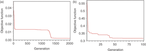
Figure 7. Evolution of the objective function for the square section with centred-hole case with the right-hand cavity. (a) Evolution of objective function S₁; (b) Evolution of objective function S₂.

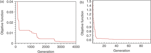
Figure 8. Cavity prediction after 2000 generations of the optimization process for the square section with centred-hole cases. (a) Top cavity case; (b) Right-hand cavity case.

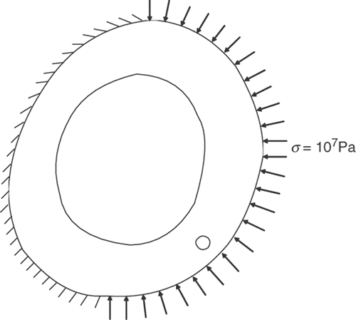
The second example shows a cross-section of the cortical bone of an adult femur. The section is roughly 4 cm in average diameter with a medullar cavity of around 2.5 cm in average diameter. The exact geometric configuration can be seen in Figure 9. The bone is assumed to be homogeneous and isotropic throughout the cross-section with a shear modulus of 3.3 GPa and a Poisson's ratio of 0.31. A small 2.5 mm cavity located on the bottom-right area of the cross-section is sought by loading the bone under normal compression of 10⁷ Pa from the right-hand side and clamping it on the left-hand side. The problem is discretized with 108 quadratic discontinuous isoparametric boundary elements.

Figure 9. Geometry and boundary conditions for the femur cross-section case.

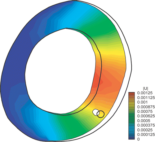
The direct problem is solved and the displacement contours are displayed in Figure 10. The displacements obtained from the direct solution are ladened with a random error of SD ±1 · 10⁻⁵ m and used as input for the inverse problem. The number of measurements employed in the optimization process is N_m = 25. A total of L = 4 point loads were employed to simulate the cavity during the first stage of the optimization processes while N_t = 8 points around the defined cluster of point loads were used to calculate the tractions during the second stage of the optimization processes.

Figure 10. Displacement contours for the femur cross-section case.

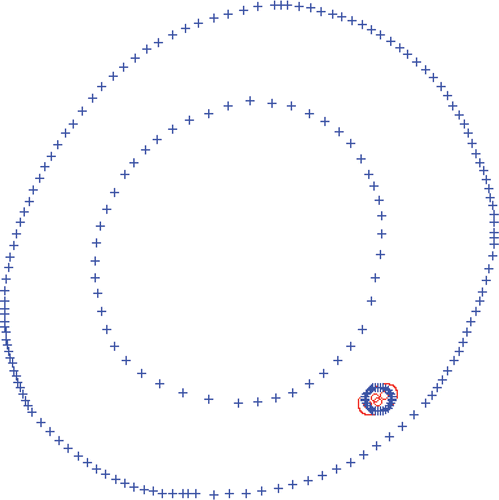
Plots of the objective functions, S₁ and S₂, evolution over the optimization process are displayed in Figure 11. The prediction of the cavity location (indicated by the dashed line) along with the location of the point loads (indicated by the small circles) is displayed in Figure 12 again revealing excellent agreement between the exact and predicted cavity location.

Figure 11. Evolution of the objective function for the femur cross-section case. (a) evolution of objective function S₁; (b) evolution of objective function S₂.

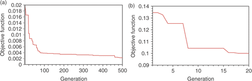
Figure 12. Cavity prediction after 500 generations of the optimization process for the femur cross-section cases.

7. Conclusions

A method for the efficient solution of the inverse optimization problem of cavity detection using a point load superposition technique in elastostatics BEM is developed in this article. Numerical examples in regular and irregular geometries demonstrate the ability of the method to successfully locate cavities in terms of their locations and size whilst using inputs ladened with simulated random error. The GA has been integrated as an optimization tool using BEM. The technique is readily applicable to the closely related problem of shape optimization, in which the condition at the cavity side may be arbitrarily specified as a design target.

Acknowledgements

The work undertaken in this project was carried out under the institutional and financial support provided by the University of Central Florida (USA), the University of Carabobo (Venezuela) and FONACIT (Venezuela).

References

- Kennon, SR, and Dulikravich, GS, 1986. Inverse design of multiholed internally cooled turbine blades, Int. J. Numer. Methods Eng. 22 (1986), pp. 363–375.
- Kubo, S, 1988. Inverse problems related to the mechanics and fracture of solids and structures, JSME Int. J. 31 (1988), pp. 157–166.
- Krapez, JC, and Cielo, P, 1991. Thermographic nondestructive evaluation: data inversion procedures, Part I: 1-D Analysis, Res. Nondestr. Eval. 3 (1991), pp. 81–100.
- Krapez, JC, Maldague, X, and Cielo, P, 1991. Thermographic nondestructive evaluation: data inversion procedures, Part II: 2-D Analysis, Res. Nondestr. Eval. 3 (1991), pp. 101–124.
- Dulikravich, GS, and Kosovic, B, 1992. Minimization of the number of cooling holes in internally cooled turbine blades, Int. J. Turbo Jet Eng. 9 (1992), pp. 226–283.
- Maldague, X, 1992. Non Destructive Evaluation of Materials by Infrared Thermography. New York: Springer-Verlag; 1992.
- Divo, EA, Kassab, AJ, and Rodríguez, F, 2004. An efficient singular superposition technique for cavity detection and shape optimization, Numer. Heat Transfer, Part B, Taylor & Francis 46 (2004), pp. 1–30.
- Ulrich, TW, Moslehy, FA, and Kassab, AJ, 1996. A BEM based pattern search solution for a class of inverse elastostatic problems, Int. J. Solids Struc. 33 (15) (1996), pp. 2123–2131.
- Kassab, AJ, Moslehy, FA, and Daryapurkar, AB, 1994. Nondestructive detection of cavities by an inverse elastostatics boundary element method, J. Eng. Anal. Bound. Elem. 13 (1994), pp. 45–55.
- Kassab, AJ, Moslehy, FA, and Ulrich, TW, 1995. "Inverse boundary element solution for locating subsurface cavities in thermal and elastostatic problems". In: Atluri, SN, Yagawa, G, and Cruse, TA, eds. Proc. IABEM-95, Computational Mechanics ‘95. Berlin, Hawaii: Springer; 1995. pp. 3024–3029.
- Ozisik, NM, and Orlande, H, 2001. Inverse Heat Transfer. New York: Taylor & Francis; 2001.
- Kurpisz, K, and Nowak, A, 1995. Inverse Thermal Problems. Southampton and Boston: Computational Mechanics Publications; 1995.
- Bonnet, M, Burczynski, R, and Nowakowski, M, 2002. Sensitivity analysis for shape perturbation of cavity or internal crack using BIE and adjoint variable approach, Int. J. Solids Struct. 39 (2002), pp. 2365–2385.
- Burczynski, T, and Beluch, W, 2001. The identification of cracks using boundary elements and evolutionary algorithms, J. Eng. Anal. Bound. Elem. 25 (2001), pp. 313–322.
- Bialecki, R, Divo, E, and Kassab, A, 2006. Reconstruction of time-dependent boundary heat flux by a BEM-based inverse algorithm, J. Eng. Anal. Bound. Elem. 30 (2006), pp. 767–773.
- Divo, EA, and Kassab, AJ, 2005. A meshless method for conjugate heat transfer problems, J. Eng. Anal. Bound. Elem. 29 (2005), pp. 136–149.
- Divo, EA, Kassab, AJ, and Ingber, MS, 2003. Shape optimization of acoustic scattering bodies, J. Eng. Anal. Bound. Elem. 27 (2003), pp. 695–703.
- Divo, EA, Kassab, AJ, Kapat, JS, and Chyu, MK, 2005. Retrieval of multidimensional heat transfer co-efficent distributions using an inverse BEM-based regularized algorithm: numerical and experimental results, J. Eng. Anal. Bound. Elem. 29 (2005), pp. 150–160.
- Mellings, SC, and Aliabiadi, MH, 1993. Brebbia, CA, and Rencis, JJ, eds. Crack Identification using Inverse Analysis, in Boundary Elements XV, Vol. 2. Boston: Computational Mechanics Publications; 1993. pp. 387–398.
- Mellings, SC, and Aliabadi, MH, 1996. Three-dimensional flaw identification using inverse analysis, Int. J. Eng. Sci. 34 (84) (1996), pp. 453–469.
- Rus, G, and Gallego, R, 2002. Optimization algorithms for identification inverse problems with the boundary element method, J. Eng. Anal. Bound. Elem. 26 (2002), pp. 315–327.
- Gallego, R, and Rus, G, 2004. Identification of cracks and cavities using the topological boundary integral equation, Comp. Mech. 33 (2004), pp. 154–163.
- Marin, L, 2005. Detection of cavities in Helmholtz-type equations using the boundary element method, J. Compu. Method. Appl. Mech. Eng. 194 (2005), pp. 4006–4023.
- Cerrolaza, M, Annicchiarico, W, and Martinez, M, 2000. Optimization of 2D boundary element models using B-splines and genetic algorithms, Eng. Anal. Bound. Elem 24 (5) (2000), pp. 427–440.
- Müller-Karger, C, González, C, Alibadi, MH, and Cerrolaza, M, 2001. Three dimensional BEM and FEM stress analysis of the human tibia under pathological conditions, J. Comp. Mod. Eng. Sci. 2 (1) (2001), pp. 1–13.
- Annicchiarico, W, and Cerrolaza, M, 2002. An evolutionary approach for the shape optimization of general boundary elements models, Electron. J. Bound. Elem. 2 (2002), pp. 251–266.
- Annicchiarico, W, and Cerrolaza, M, 2004. A 3D boundary element optimization approach based on genetic algorithms and surface modeling, Eng. Anal. Bound. Elem. 28 (11) (2004), pp. 1351–1361.
- Annicchiarico, W, Martínez, G, and Cerrolaza, M, 2005. Boundary elements and B-spline modeling for medical applications, J. App. Math. Mod. 31 (2) (2005), pp. 194–208.
- Martínez, G, and Cerrolaza, M, 2006. A bone adaptation integrated approach using BEM, J. Eng. Anal. Bound. Elem. 30 (2006), pp. 107–115.
- Brebbia, CA, and Dominguez, J, 1989. "Boundary element, An introductory course". In: Computational mechanics Publ. New York: Boston, (co-published with McGraw-Hill; 1989. pp. 134–250.
- Kane, JH, 1994. Boundary Element Analysis in Engineering Continuum Mechanics. Englewood Cliffs, New Jersey: Prentice Hall; 1994. p. 07632.
- Goldberg, D, and Richarson, J, 1987. Genetic algorithms with sharing for multimodal function optimization, Proceedings of the Second International Conference on Genetic Algorithms and Their Applications (1987), pp. 41–49.
- Goldberg, D, 1989. Genetic Algorithms in Search, Optimization, and Machine Learning. Reading, MA: Addison-Wesley; 1989.