Identification of thermal conductivity and the shape of an inclusion using the boundary elements method and the particle swarm optimization algorithm

Abstract

Temperature measurements from the exterior boundary of a two-dimensional solid body containing an inclusion, under steady state conditions, are used to estimate the thermal conductivity and the shape of the inclusion. The particle swarm optimization algorithm (PSO), coupled with the boundary elements method, is used in this identification problem. A fitness function which is the summation of the squared differences between the measured and calculated temperatures at the locations on the exterior boundary is minimized. To avoid trapping into the local optimum points, the PSO algorithm which is a global optimization method is used instead of local optimization methods. The credibility of the PSO algorithm and its effectiveness in solving inverse problems is investigated. The effect of measurement errors and the size of the inclusion on the estimation process will be addressed.

Keywords:

• inverse heat conduction problem
• inclusion
• boundary element method
• particle swarm optimization

1. Introduction

The characterization of the internal structure of a solid body containing an inclusion of unknown shape and thermal properties is investigated. This shape estimation problem involves the study of inverse problems which usually imply the identification of inputs from outputs. In direct problems, the governing differential equations in a domain with known shape, along with the boundary conditions and material properties is solved for temperatures. In inverse problems, material properties or geometric parameters defining the domain of the problem are unknown. This inverse problem is solved for unknown geometric parameters or material properties using temperature measurements on the exterior boundary.

The geometric parameter estimation 1 and energy generation 2 are some of the applications of the inverse problems. For the non-linear inverse problem investigated here, an iterative scheme is required. Thus the boundary element method (BEM), which requires only the discretization of the boundary, must be employed in order to avoid the costly and unnecessary task of grid generation for the entire multiply connected domain at each iteration 3.

There are several optimization methods for the solution of inverse problems. The most common methods of optimization, i.e. local optimization methods are based on the gradient of some defined fitness function. Although in some cases these methods converge to the correct answer, they often get stuck in local optimum points, therefore a good initial guess of the unknown parameters is needed. This inverse problem is ill-posed and very sensitive to the errors involved in experimental measurements. To correct this problem, regularization functions like Tikhonov 4 and Beck 5 are employed. Although each of these methods have some advantages, none of them are completely effective.

The inverse problem has been solved to estimate optimal shape of cooling passages in turbine blades 6. Elliptic functions have been used to estimate the geometry of cooling passages using inverse heat conduction method 7. The thermal conductivity, location and radius of one circular inclusion inside a two-dimensional solid body have been estimated in 8. The extension to this study is to estimate the thermal conductivity, location and radius of two circular inclusions inside a solid body 9.

There are several optimization methods implemented to optimize different systems. One of these methods is the particle swarm optimization algorithm (PSO). The PSO algorithm is a global and novel multi-agent optimization system (MAOS) inspired by social behaviour metaphor. It has been shown that the PSO is an effective method used in many optimization problems, and does not have some of the difficulties involved in the local optimization methods 10.

The present article assumes a two-dimensional body containing a single inclusion, but the method of analysis is not limited in principle. Extension to three-dimensional problems and more complex internal structures is straightforward, but the effectiveness of different optimization methods implemented in many inverse problems needs further study. Nonetheless, the success of the technique demonstrated here shows great promise for application in the area of non-destructive evaluation.

2. The direct problem

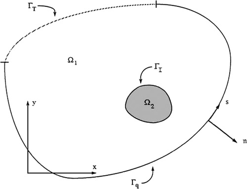
The differential equation representing steady state heat transfer through an isotropic, homogeneous, two-dimensional region, Ω, is (1) where T(x,y) is the temperature, k is the thermal conductivity and ∇² = (∂²/∂x²)  + <br/ > (∂²/∂y²). The boundary conditions can be written as: (2) (3) where T₀(s) and q₀(s) are specified function and the boundary of region Ω is given as Γ = Γ_T + Γ_q, n is the outward unit normal direction to Γ, q is the heat flux in the n direction and s is a coordinate along the boundary as shown in Figure 1.

Figure 1. Plane inhomogeneous body.

The above problem is solved by the following BEM algorithm. The boundary integral equation for a constant property, steady-state heat conduction problem without heat generation term can be derived as 11: (4) where i is a point on Γ or in Ω (α = 1 if i is in Ω, α < 1 if i is on Γ, α = 0.5 if Γ is smooth at i), T* is the fundamental singular solution and q* is the normal derivative of T*. In two dimension , where r is the distance from point i to any point on Γ.

Subdividing the boundary Γ into linear isoparametric elements, Equation (4) is written in matrix form as: (5) where {T} is a vector containing temperatures at NE boundary nodes, {q} is a vector containing two values of flux at each boundary node, i.e. one heat flux ‘before’ the node and one ‘after’ the node, [H] and [G] are geometry-dependent matrices.

For multiply connected domain, the domain Ω is divided into two subdomains Ω₁ and Ω₂, each having its own thermal conductivity and Equation (5) is reapplied to each subdomain. For two subdomains: or (6) Equation (6) is then reduced by imposition of interface conditions. At a point i on the interface boundary Γ_I, the interface conditions are: (7) where continuity of heat flux at the interface nodes is assumed.

Finally after all boundary conditions are imposed, the system of equations is written in the form: (8) which is solved for . The column vector contains the values of unknown temperatures and heat fluxes at the outer boundary nodes as well as all temperatures and heat fluxes at the interface boundary nodes.

3. The inverse problem

In the direct problems, the governing differential equation, geometry, material properties and the boundary conditions are given and the unknown boundary data is computed. In the inverse problem the geometric features and/or material properties are unknown, but some of the unknown boundary data can be measured and used as additional information necessary to estimate the unknown input parameters.

A body that is known to contain an inclusion with unknown shape and thermal conductivity is considered. These unknown parameters are determined by using the measurement of temperatures on the portion of the boundary where fluxes are prescribed.

The following column vectors are introduced:

	=	= a column vector containing M measured boundary temperatures.
	=	= a column vector containing the same M boundary temperatures, computed using the BEM.
	=	= a column vector containing N unknown parameters to be estimated and is written as: (9)

where k is the thermal conductivity of the inclusion, (x_c,y_c) are the coordinates of the centre of the inclusion, and r_i are the radial distances of n nodes on the interface boundary of inclusion to (x_c,y_c) as shown in Figure 2.

Figure 2. Geometric parameters and problem modelling.

The fitness function is defined as the sum of the squared differences between measured and computed temperatures as follows: (10) where ‘∧’ denotes the estimated values of the unknown parameters.

4. Particle swarm optimization

4.1. Background of PSO

The implicit rules adhered to by birds, flocks and fish travelling in large groups, enabling them to move synchronized, without colliding, resulting in an amazing choreography, was studied and simulated by several scientists 12. In simulations, the movement of the flocks was an outcome of the individuals (birds, fish, etc.) efforts to maintain an optimum distance from their neighbouring individuals 13.

The social behaviour of animals, and in some cases of humans, is governed by similar rules 14. There is a general belief, and numerous examples coming from the nature that enforces the view, i.e. sharing of information among the individuals of a population may provide an evolutionary advantage. This was the core idea behind the development of the PSO 13.

4.2. The PSO algorithm

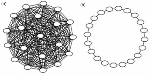
According to the above-mentioned background, Kennedy and Eberhart developed the PSO concept 9. The PSO algorithm is an iterative method and involves initializing a number of vectors that are called ‘particles’, randomly within the search space of the fitness function. These particles are collectively known as the ‘swarm’. Each particle represents a potential solution to the problem expressed by the fitness function. During each time step, the fitness function is evaluated to establish the fitness of each particle using its position as input. Fitness values are used to determine which positions in the search space are better than others. Particles are then made to ‘fly’ through the search space being attracted to both their personal best position as well as the best position found by some other particle. Various methods have been used to identify ‘some other particle’ to influence the individual. The two most commonly used methods are known as gbest and lbest (Figure 3). In the gbest population, the trajectory of each particle's search is influenced by the best point found by any member of the entire population. The lbest population allows each individual to be influenced by some smaller number of adjacent members of the population array. Typically lbest neighbourhoods comprise of exactly two neighbours, one on each side: a ring lattice.

Figure 3. gbest (left) and lbest sociometric pattern.

Now, suppose that the search space is D-dimensional, then the i-th particle of the swarm can be represented by a D-dimensional vector X_i = (x_i1,x_i2,…,x_iD)^T. The velocity (position change) of this particle, can be represented by another D-dimensional vector V_i = (v_i1,v_i2,…,v_iD)^T. Modification of the agent position is realized by the position and velocity information. Each agent knows its best value so far (pbest) and its X_i position. This information is analogy of personal experiences of each agent. Moreover, each agent knows the best value so far in the group (gbest) or in their neighbourhoods (lbest) among pbests. This information is analogy of knowledge of how the other agents around them have performed. Namely, each agent tries to modify its position using the following information:

•	The current positions Xi
•	The current velocities Vi
•	The distance between the current position and pbest
•	The distance between the current position and gbest or lbest

This modification can be represented by the concept of velocity.

4.2.1. Gbest model

The gbest model offers a faster rate of convergence at the expense of robustness 13. This model maintains only a single ‘best solution’, called the global best particle, across all the particles in the swarm. This particle acts as an attractor, pulling all the particles towards it. Eventually all particles will converge to this position, so if it is not updated regularly, the swarm may converge prematurely and trap in local optima. The update equations for gbest and V are as follows: (11) (12) i = 1,2,…,N where N is the size of the swarm; d = 1,2,…,D where D is the dimension of search space, where iTer_max is the maximum number of iterations, w is the inertia weight, the acceleration coefficients c₁ and c₂ are two positive constants called the cognitive and social parameter respectively, r_1id and r_2id are random numbers uniformly distributed within the range [0, 1]. Note that gbest is called the global best position, and belong to the particle referred to as the global best particle.

The current position (searching point in the solution space) can be modified by the following equation: (13) (14) where and are lower and upper bound of search space of particles in d-th dimension, respectively. Since there was no actual mechanism for controlling the velocity of a particle, it was necessary to impose a maximum value on it, i.e. . If the velocity exceeded this threshold, it was set equal to . This parameter proved to be crucial, because large values could result in particles moving past good solutions, while small values could result in insufficient exploration of the search space. The value of is usually chosen to be k × x_d,max, with 13. In this article, to cover all search space by particles, where k = 1.0 is used.

Equation (12) is used to determine the i-th particle's new velocity at each iteration, while Equation (13) provides the new position of the i-th particle adding its new velocity to its current position. The performance of each particle is measured according to a fitness function which is problem dependent. In optimization problems, the fitness function is usually identical with the fitness function under consideration, i.e. Equation (10).

4.3. The parameters of the PSO

The role of the inertia weight, w, in Equation (12) is considered critical for the PSO's convergence behaviour. The inertia weight is employed to control the impact of the previous history of velocities on the current one. Accordingly, the parameter w regulates the trade-off between the global and local exploration abilities of the swarm. A large inertia weight facilitates global exploration (searching new areas), while a small one tends to facilitate local exploration, i.e. fine-tuning the current search area. A suitable value for the inertia weight, w usually provides balance between global and local exploration abilities and consequently results in a reduction of the number of iterations required to locate the optimum solution. Initially, the inertia weight was constant. However, experimental results indicated that it is better to initially set the inertia to a large value, in order to promote global exploration of the search space, and gradually decrease it to get more refined solutions. Thus, Shi and Eberhart 15, made a significant improvement in the performance of the PSO with a linearly varying inertia weight over the generations, which linearly vary from at the beginning of the search to at the end. Thus, the following weighting function is usually utilized in Equation (12). (15) where and are initial and final inertia weight, respectively, and n is the current iteration number.

The parameters c₁ and c₂, in Equation (12), are not critical for PSO's convergence. However, proper fine-tuning may result in faster convergence and the alleviation of local minima. An extended study of the acceleration parameter in the first version of PSO is given in 16. As default values, c₁ = c₂ = 2 were proposed, but experimental results indicate that c₁ = c₂ = 0.5 might provide even better results. Recent work reports that it might be even better to choose a larger cognitive parameter, c₁, than a social parameter, c₂, but with 17.

The parameters r₁ and r₂ are used to maintain the diversity of the population, and they are uniformly distributed in the range [0, 1].

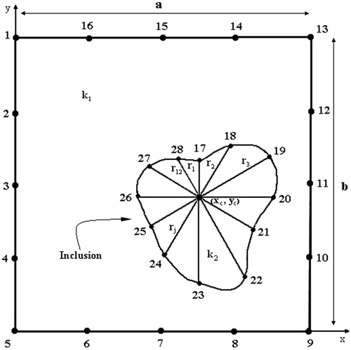
In this article, the initial population of swarm should be chosen such that all the unknown parameters, i.e. Equation (9) are represented. For this reason, particles which include thermal conductivity and x − y coordinates of the centre of the inclusion and a number of radiuses needed to estimate the shape of the inclusion are chosen as the initial population. The first three agents do not have any limit in their values and they pick a number between lower and upper limitation. But the radius should be such that the boundary of the inclusion remains within the domain of the problem. Therefore if the inclusion is assumed to be inside a rectangular domain with dimensions of a and b as shown in Figure 2, then the radius should be bounded by the following equations: (16) If the radius is within the above limits, it will be chosen as the candidate answer; otherwise another random value for radius will be tested.

This condition must hold for all iterations, therefore in the next iteration after updating the parameters according to Equation (13), the geometric constraint of the inclusion radii defined by a function is explored using Equation (16). If Equation (16) holds for the estimated radius, then it is a suitable one, otherwise it is set equal to or . It should be noted that the constraints for the third agent and its following (radii) will be different for each particle.

5. Computational procedure

Using MATLAB, a computer program is developed to compute the unknown parameters using the PSO algorithm. The computational procedure for the solution of this problem may be summarized as follows:

Step 1

Forming the initial population of swarm within a defined limit by Equation (9).

Step 2

Computing the fitness function for each particle from Equation (10).

Step 3

Examination of the stopping criterion.

Step 4

Specification of pbest and gbest.

Step 5

Computing the speed of each particle from Equation (12).

Step 6

Modifying the new values of particles by Equation (13) and returning to Step 2.

6. Results and discussions

6.1. Analysis model

An inclusion of unknown thermal conductivity and geometric shape is located somewhere inside a rectangular solid body of size (1  × 1 m²). To simulate the experimental measurements of temperatures, the Steel body Ω₁ with k = 73 containing an Aluminium inclusion (k = 164) with the shape of an ellipse or a pear are considered under steady state heat transfer. The parametric equation of ellipse and pear are as follows: (17) (18)

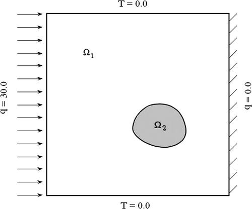
The outer boundary is divided into 16 linear elements and the interface boundary is divided into 12 elements. The boundary conditions and domains of the problem are shown in Figure 4.

Figure 4. Plane inhomogeneous body with boundary conditions.

The temperature measurements are obtained on the portion of the boundary where flux is specified as boundary condition. The temperatures computed on the left and right sides of this model, i.e. nodes 2–4 and 10–12 as shown in Figure 2, where flux boundary condition is specified are used as experimental results. The ‘experiment’ is simulated as follows. The body is analysed by BEM using the exact value of the parameters and unknown boundary temperatures and heat fluxes are computed. These computed values are then used as the experimental results.

The global neighbourhood procedure of the PSO algorithm is used in this investigation. The appropriate values of the PSO parameters are obtained by examining different values of these parameters and making many trial and error runs. The values are r₁ = r₂ = 1.0, and the size of swarm (N_S) equals 1000. These values are appropriate since they result in the best rate of convergence to a correct solution and are kept constant throughout this investigation.

A relative percent error coefficient for analysing the results is defined as follows: (19) where x_act is the actual value of the unknown parameter and x_est is the estimated value of the unknown parameter and N is the number of unknown parameters. The accuracy of results is the average value obtained from 10 different runs.

The unknown parameters are defined as 12 radial distances from centre to each nodal locations on the inclusion boundary, along with (x_c,y_c), coordinates of centre and thermal conductivity of the inclusion. Therefore, the total of 15 parameters (N = 15) are estimated. The thermal conductivity of the inclusion is considered within the range of .

The stopping criteria for the PSO algorithm is or . Usually for error-free measurements of temperatures, the first criterion is satisfied, and for the erroneous experimental measurements of temperatures the second criteria is satisfied.

The reason for the selection of these stopping criteria is based on our knowledge of the characteristics of the real parameters and by playing with the value of the parameters and by trial and error. In PSO procedure after a number of iterations, similar swarms are obtained which is taken to be the best converged results. When error-free measurements are used, often the first criterion, i.e. gives accurate converged value of estimated parameters, but when erroneous measurements are used, since random errors are added to the temperatures, the possibility of reaching this tolerance does not exist and with more iterations, improvements of results is not obtained.

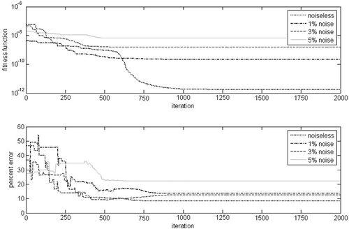
Figure 5 shows sample of the fitness function values and percent error for four random runs using errorless and also erroneous measured data with 1, 3 and 5% errors, and elliptic shape inclusion located at the centre of the domain, i.e. (0.5, 0.5). The PSO algorithm has the size of swarm (N_S) equals 1000 and it runs up to 2000 iterations. It is observed that in both cases after a number of iterations, the value of the fitness function and percent error become stable and reach the level of noise. The algorithm even proceeds with more iterations, but improvements in the results are not noticeable. Therefore with regard to Figure 5 and to avoid long computational time, has been chosen as an optimum choice.

Figure 5. Sample of the fitness function values and percent error as function of iteration.

6.2. The number of experimental measurements needed

The number of measurements, i.e. M equal to one, two and six measurements of temperature are used in this investigation, respectively, to identify the shape of an elliptic inclusion located at the centre of the domain, i.e. (0.5, 0.5). One location has been chosen randomly among nodes 2–4 and 10–12, then two locations are chosen randomly among the same nodes on each side of the model and finally temperatures measured at all six locations are used to estimate the parameters. The estimation is stopped after 1000 iteration of the PSO algorithm. The fitness function, f(x), given by Equation (10) converges to a very small number in all of the cases investigated.

In some cases, the converged value of parameters are not acceptable and are considered wrong, this happens since there is no unique solution for this ill-posed inverse problem: in other words it is possible that different shapes of inclusion give the same temperature distribution on the exterior boundary.

Table 1 shows the average percent error found by using Equation (19) from converged cases and also the average value of the fitness function from Equation (10) for 10 different runs.

Table 1. Comparison of the fitness function and the actual error function.

Number of measurements	1 Node	2 Nodes	6 Nodes
f(x)	3.6 × 10^− 17	8.9 × 10^− 13	2.7 × 10^− 10
% Error	56.14%	25.43%	12.03%

It is observed that using one and two measurements, the average value of the fitness function is less than the case when six measurements are used but the percent error is less for the case of six measurements, so we use all six temperatures. It is concluded that the value of the fitness function cannot be a good criterion of convergence. All six temperatures at nodes 2–4 and 10–12 are used for the remaining part of this investigation.

6.3. Influence of inclusion location on the estimation

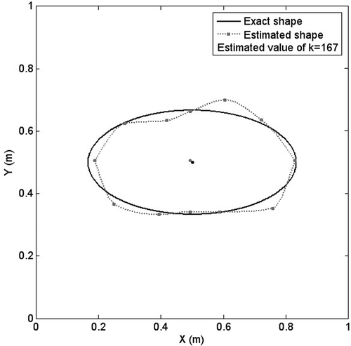
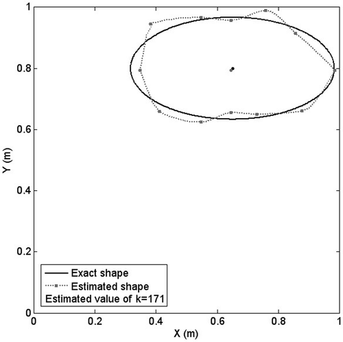
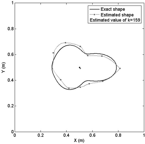
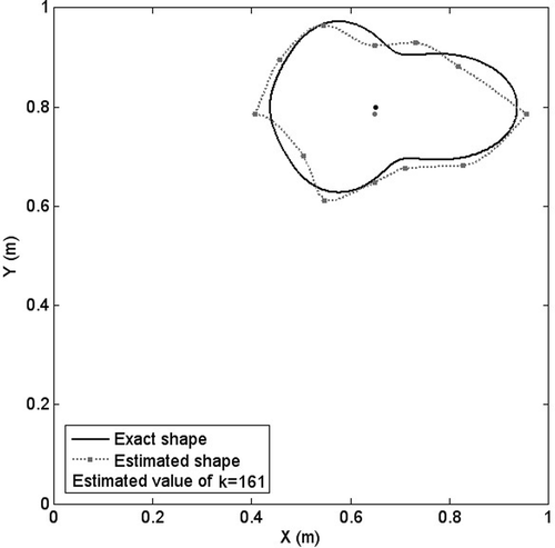
Next, the effect of inclusion location inside the body is investigated. Two cases of both elliptic and pear-shaped inclusions are considered. First, the x − y coordinates of the centre point of the inclusion is set at (0.5, 0.5) and the unknown parameters are estimated, then the centre point is chosen at (0.65, 0.8) which is closer to the outer boundary. The algorithm estimates all the unknown parameters successfully with about 88% accuracy for both cases. But the number of iterations and therefore the computational time increases considerably for the case of the centre point at (0.65, 0.8), because this location is closer to the outer boundary and according to the limitations and constraints of the PSO algorithm in estimating the radiuses, the computational time increases up to there times. The sample results are shown in Figures 6–9.

Figure 6. Elliptic inclusion identification with centre point (0.5 , 0.5).

Figure 7. Elliptic inclusion identification with centre point (0.65, 0.8).

Figure 8. Pear shaped inclusion identification with centre point (0.5 , 0.5).

Figure 9. Pear shaped inclusion identification with centre point (0.65, 0.8).

6.4. The effect of inclusion size on convergence

To investigate the effect of the inclusion size, different sizes of elliptic shape inclusion with equation A(x − 0.5)² + B(y − 0.5)² = 1 are considered. The results are shown in Table 2. The percent error is the average value of percent error for 10 different runs. It is shown that very small inclusion or very large ones are difficult to identify. For a small inclusion, the measured boundary temperatures are less sensitive to the existence of an inclusion and for a very large inclusion, its boundary interferes with the outer boundary of surrounding body and the limitations on the value of radiuses, i.e. Equation (16), makes it difficult to identify the inclusion with good accuracy.

Table 2. Influence of inclusion size on the estimation.

Case No.	A	B	% Area	% Error
1	6	25	23.40	18.14
2	9	36	17.46	12.03
3	16	49	11.22	11.22
4	25	64	7.86	13.41
5	36	81	4.84	15.37

6.5. The effect of measurement errors on the estimation process

Next, the effect of inevitable experimental errors on the estimation process of a pear-shaped inclusion is investigated. For simulation of this case, random errors are added to the computed temperatures with exact values of parameters, and these are taken to be the 'measured’ data. The statistical assumptions regarding the introduced errors are additive, non-correlated, normally distributed and have zero mean and constant variance. The measured data or erroneous temperatures are generated according to: (20) where σ is the error, and m is the iteration count.

Since the PSO algorithm is only a direct search method, small experimental errors do not have much effect on its performance. The unknown parameters are estimated by experimental measurements with 1–5% errors. Since the errors are added to the computed displacements randomly, for each percent error 10 combinations of different erroneous temperatures are considered. The sample results are presented in Table 3.

Table 3. The influence experimental errors on the estimation process.

Percent error (%)	Average % error	Minimum % error	Maximum % error
1	13.74	12.18	15.67
2	15.53	11.96	18.28
3	18.10	12.18	24.18
4	19.21	16.11	22.63
5	23.26	15.85	29.91

As shown in Table 3, the third and fourth columns give the minimum and maximum percent error computed using Equation (19). With increasing the percent random errors in measurements, the percent error and the value of coefficient variable also increases. It is observed that for 5% error in experimental measurements, the estimation of the inclusion converges to non-realistic values.

7. Conclusions

The inverse application of BEM to estimate the thermal conductivity and the shape of an inclusion using the PSO algorithm proves to be an effective optimizing method. The following advantages of the above numerical scheme are observed:

•	Estimation does not need an initial guess of the unknown parameters.
•	Simultaneous estimation of the geometric and thermal conductivity of an inclusion is possible with good accuracy.
•	Convergence is achieved even with inevitable measurement errors.

Acknowledgements

The authors express their appreciation to the research council of the Moshanir Consulting Engineering Company and research council of the Yazd University for the financial support of this work.

References

- Huang, CH, and Shih, CC, 2006. A shape identification problem in estimating simultaneously two interfacial configurations in a multiple region domain, Appl. Therm. Eng. 26 (2006), pp. 77–88.
- Huang, CH, Yeh, CY, and Orlande, HRB, 2003. A non-linear inverse problem in simultaneously estimating the heat and mass production rates for chemically reacting fluid, Chem. Eng. Sci. 58 (2003), pp. 3741–3752.
- Lesnic, D, Elliott, L, and Ingham, B, 1996. Application of boundary element method to inverse heat conduction problems, Int. J. Heat Mass Transfer. 39 (1996), pp. 1503–1517.
- Engl, HW, and Zou, J, 2000. A new approach to convergence rate analysis of Tikhonov regularization for parameter identification in heat conduction, Inverse Probl. 16 (2000), pp. 1907–1923.
- Ring, W, 2001. A first-order sequential predictor-corrector regularization method for ill-posed Volterra equations, SIAM J. Num. Anal. 38 (2001), pp. 2079–2102.
- Dulikravich, GS, and Martin, TJ, 1992. Inverse design of super elliptic cooling passages in coated turbine blade airfoil, J. Thermophys. Heat Transfer. 8 (1992), pp. 288–294.
- Huang, CH, and Suing, TY, 1999. An inverse design problem of estimating optimal shape of cooling passages in turbine blades, Int. J. Heat Mass Transfer. 42 (1999), pp. 4307–4319.
- Khodadad-Saryazdi, M, and Altiero, NJ, Third Annual Inverse Problems in Engineering Seminar. Presented at Characterization of the interior of an inhomogeneous body using surface temperature and/or heat flux measurements. East Lansing, Michigan, USA, 1990.
- Khodadad-Saryazdi, M, Seyed-Rihani, SA, and Abbasiyan, M, Estimation of the parameters related to impurities inside solid bodies using the inverse and boundary element methods. Presented at 10th Annual (International) Conferences of Mechanical Engineering, ISME2002. 24–26 May, 2002.
- Kennedy, J, and Eberhart, RC, Particle Swarm Optimization. Presented at Proceedings of the International Conference on Neural Networks. Perth, Australia, 1995.
- Brebbia, CA, and Dominguez, J, 1989. Boundary Elements: An Introductory Course. Southampton: Computational Mechanics Publications; 1989.
- Heppner, F, and Grenander, U, 1990. "A stochastic nonlinear model for coordinate bird flocks". In: Krasner, S, ed. The Ubiquity of Chaos. Washington, DC: AAAS Publications; 1990.
- Eberhart, RC, Simpson, P, and Dobbins, R, 1996. Computational Intelligence PC Tools. Boston, MA: Academic Press; 1996.
- Wilson, EO, 1975. Sociobiology: The New Synthesis. Cambridge, MA: Belknap Press; 1975.
- Shi, Y, and Eberhart, RC, 1998. "Parameter selection in particle swarm optimization". In: Porto, VW, Saravanan, N, Waagen, D, and Eiben, AE, eds. Evolutionary Programming VII. New York: Springer; 1998. pp. 611–616.
- Kennedy, J, 1998. "The behavior of particles". In: Porto, VW, Saravanan, N, Waagen, D, and Eiben, AE, eds. Evolutionary Programming VII. Berlin, Germany: Springer; 1998. pp. 581–590.
- Carlisle, A, and Dozier, G, 2001. An off-the-shelf PSO. Presented at Proceedings of the Particle Swarm Optimization Workshop.