Inverse probabilistic modelling of the sources of uncertainty: a non-parametric simulated-likelihood method with application to an industrial turbine vibration assessment

Abstract

As probabilistic analyses spread in industrial practice, inverse probabilistic modelling of the sources of uncertainty enjoys a growing interest as it is often the only way to estimate the input probabilistic model of unobservable quantities. This article addresses the identification of intrinsic physical variability of the systems. After showing its theoretical differences with the more classical data assimilation or parameter identification algorithms, this article introduces a new non-parametric algorithm that does not require linear nor Gaussian assumptions. This technique is based on the simulation of the likelihood of the observed samples, coupled with a kernel method to limit the number of physical model runs and facilitate the subsequent maximization. It is implemented inside an industrial application in order to identify the key parameter that controls the vibration amplification of steam turbines. Hence, experimental resonance frequencies observations are used to adjust the probabilistic model of the unobservable manufacturing imperfections between theoretically identical units.

Keywords:

• uncertainty
• identification
• data assimilation
• maximum likelihood
• probabilistic non-parametric method
• vibrations

1. Introduction

A growing number of industrial modelling studies include some treatment of the numerous sources of uncertainty affecting their results. Uncertainty treatment in physical, environmental or risk modelling is the subject of a long-standing body of academic literature 1–5. It is of particular industrial importance in the field of power generation, where a large number of applications, beyond the traditional reliability domain, have gradually included some uncertainty treatment, including in particular: (i) nuclear safety studies involving large scientific computing (thermo-hydraulics, mechanics, neutronics, etc.) or Probabilistic Safety Analyses (PSA); (ii) environmental studies (flood protection, effluent control, etc.).

For most of those applications, at least partial probabilistic modelling of the uncertainties is considered, although deterministic uncertainty treatment or alternative non-probabilistic approaches keep their share. Apart from the important uncertainty propagation issues in the context of often complex and high-CPU demanding scientific computing, one challenge regards the quantification of the sources of uncertainties or uncertainty modelling: this refers to the issue of choosing statistical models (mostly pdf, probability distribution functions) in an accountable manner for the input variables such as uncertain material properties, industrial processes or natural aleatory phenomena (wind, flood, temperature, etc.). Key difficulties arise with the highly limited sampling information directly available on the input variables in any real-world industrial case: real samples in industrial safety or environmental studies, if any, often fall below the critical size required for stable statistical estimation.

A tempting strategy is to integrate indirect information, i.e. data on other parameters that are more easily observable and linkable to the uncertain variables of interest through a physical model. This involves the inversion of a physical model to transform the indirect information, and is acknowledged to have quite a large industrial potential in the context of rapid growth of industrial monitoring and data acquisition systems: on a nuclear reactor, large flows of data are generated by multiple physical monitoring (e.g. pressure, temperature, fluencies, etc.) thereby documenting the intrinsic physical variability of the systems. Proper model calibration and inverse algorithms could theoretically supply information on the unobservable sources of uncertainties that are at the root of the process, e.g. thermal exchange coefficients, basic nuclear parameters, etc. One of the big issues in practice is to limit the number of (usually large CPU-consuming) physical model runs inside the inverse algorithms to a reasonable level.

As will be seen later on, although connected to classical data assimilation, parameter identification model calibration or updating techniques, inverse probabilistic modelling shows distinctive features: it regards the way uncertainty sources are conceptually acknowledged and mathematically modelled on unknown model parameters or model uncertainty. While inverse probabilistic techniques are already old 6–8, it may not be until quite recently that full probabilistic inversion was considered, in the sense that the distribution of intrinsic (or irreducible, aleatory) input uncertainty or variability is searched.

Indeed, a long debate 3,5,9–11 originating from the first large risk assessments in the US nuclear domain has ended up with the importance of distinguishing two types of uncertainty: namely the epistemic (or reducible, lack of knowledge, etc.) type referring to uncertainty that decreases with the injection of more data, modelling or number of runs and the aleatory (or irreducible, intrinsic, variability, etc.) type for which there is a variation of the true characteristics that may not be reduced by the increase of data or knowledge. Classical data assimilation 8,12 or parameter identification techniques (for instance 13–15) involve the estimation of input parameters (or initial conditions in meteorology) that are unknown but physically fixed; this is naturally accompanied by estimation uncertainty for which a variance may be computed. However, such an estimation uncertainty happens to be purely epistemic or reducible because it will decrease with the injection of larger observation samples 16. This is not satisfactory in the case of intrinsically uncertain or variable physical systems, i.e. for which the input values not only suffer from lack of knowledge, but also vary from one experiment to another or from one unit to another. Regarding the full probabilistic inversion techniques adapted to intrinsically variable inputs, Kurowicka and Cooke 17 suggested some algorithms identifying the pdf of the inputs (X) when the pdf of the observable outputs (Y = G(X)) is supposed to be elicited by experts who are asked to provide a few quantiles (usually 5%, 50%, 95%), which is however hardly possible with complex industrial codes; De Crécy 18 suggested the CIRCE algorithm (derived from the older and more general Expectation-Maximization (EM) statistical algorithm 19) that allows the inference of X co-variances from an observation sample on Y. This last algorithm is still being used with complex nuclear thermo-hydraulic codes, but under limiting Gaussian and/or linear assumptions.

This article is structured as follows. It will first recall in Section 2 the generic setting of an industrial uncertainty study, and mathematically position the rationale for inverse probabilistic modelling. The theoretical review of the corresponding estimation problem is the subject of Section 3: a clear difference is drown between data assimilation, parameter identification and ‘full probabilistic inversion’ techniques as regards the identification of epistemic and aleatory uncertainty and the existing algorithms are reviewed. Subsequently, a new algorithm combining likelihood approximation and a dedicated non-parametric setting is introduced in Section 4. Lastly, Section 5 explains the industrial application to a steam turbine vibration prediction problem. Conclusions and some further research needed are outlined in Section 6.

2. The generic issue of uncertainty treatment in industry and the rationale for inverse probabilistic modelling

2.1. Industrial system models considered

Quantitative uncertainty assessment in the industrial practice typically involves 20,21:

•	a pre-existing physical or industrial system or component lying at the heart of the study, that is represented by a pre-existing model,
•	inputs, affected by a variety of sources of uncertainty,
•	an amount of data and expertize available to calibrate the model and/or assess its uncertainty,
•	industrial stakes and decision-making that motivate the uncertainty assessment more or less explicitly. They include: safety and security, environmental control, financial and economic optimization, etc. They are generally the purpose of the pre-existing model, the output and input of which help handling in a quantitative way those stakes within the decision-making process.

The pre-existing system may refer to a very wide variety of situations, such as: a metrological chain, a mechanical structure, a maintenance process, an industrial or domestic site threatened by a natural risk, etc. Talking about the quantitative study of uncertainties, that system will generally be modelled by a single numerical system model or a chain of models: anything from the straightforward analytical formulae to coupled 3D finite element models, etc. standing as a numerical function linking output variables (noted m) to a number of continuous or discrete input variables or parameters, where (see Equation (1) and Figure 1):

Figure 1. Variables and structure of the pre-existing model.

•	some input variables (noted x = (xi)i=1 … p, underlining denoting vectors throughout this article) are uncertain, subject to randomness, variability, lack of knowledge, errors or any sources of uncertainty,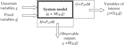
•	while other inputs (noted d) are fixed, either being well known (e.g. controlled experimental factors for calibration, design choices, etc.) or being considered to be of secondary importance with respect to the output variables of interest.

(1) Note that computation of the pre-existing model for a point value (x, d) (i.e. not uncertain at all) may require a very variable CPU time: depending on the case, from 10⁻⁴ s to several days for a single run.

Within the potentially large number of raw outputs of the models, it is useful to sub-distinguish two categories:

•

the model output variables of interest that are eventually important for the decision criteria are included formally within the vector z = (zv)v=1… r: most of the time, z is a scalar (z) or a small-size vector (<5 components) since the decision-making process involves essentially one or few variables of interest such as: a physical margin to failure, a net cost, an cumulated environmental dose or a failure rate in risk analysis.

•

the model observable outputs, upon which some data is available albeit potentially subject to noise caused by measurement errors. Referring to physical variables or degrees of freedom (DOF) that can be easily instrumented or observed, they often differ from the outputs associated with the eventual decision process (z): they will be noted y = (yl)l=1… m.

Basically y and z can be viewed as simple projections of the raw output vector m; in some studies however, some limited post-treatments are compounded to the raw model outputs in ways that differ between the variables of interest (e.g. standardizing a mechanical margin criterion) and the observable outputs (e.g. volume averaging due to metrological device) so that we would formally note: (2) (3) where P_d and P_o refer to deterministic operators that can be a bit more complex than simple projections.

2.2. Probabilistic uncertainty studies

While literature has discussed to a large extent the pros and cons of various probabilistic or non-probabilistic paradigms 4,11,21–23, it is assumed in this article that probabilistic uncertainty treatment is acceptable for the cases considered: meaning that decision criteria will generally involve the consideration of some peculiar ‘quantities of interest’ on the distribution Z representing uncertainty in a probabilistic sense on the output variables of interest, such as: variance or coefficient of variation on one or more outputs, confidence intervals on the variables of interest or probabilities of exceeding a safety threshold, etc.

Formally, consider thus a probabilistic setting, involving a sample space X (generally part of ℜ^p but some components may be discrete) for the input variables x from a probability space structure in which: (4) whereby f_X indicates a joint probability distribution function (pdf) associated to the vector of uncertain inputs X (capital letters denote random variables). Parameters of f_X are grouped within the vector θ_X: they include parameters of position, scale and shape, or moments of marginal laws, coefficients of correlations (or parameters of the copula function) or even extended parameters of a non-parametric kernel model. Image measures for spaces Y and Z (generally parts of ℜ^m and ℜ^r) are deduced, assuming the measurability of the pre-existing models H(.) and G(.). The following formulae link the random vectors Y and Z to X and d: (5) (6) Once this specification step is complete, uncertainty studies typically involve the following steps 20: the modelling of uncertainty sources, i.e. the estimation of the distribution f_X (with its parameters θ_X) either through direct statistical data or expertize treatment or through inverse methods; hence the uncertainty propagation, i.e. the computation of given output quantities of interest (e.g. c_z = var Z or c_z = P(Z > z_s)) or sometimes of the whole pdf of Z given the full knowledge of the input pdf f_X. Importance ranking or sensitivity analysis 22–27 may then be considered to rank or apportion the contributions of uncertain inputs (Xⁱ)_{i=1 … p} to a given output quantity of interest c_z (which is generally variance). These last steps involve a large number of probabilistic and numerical techniques, such as simulation, optimization, regression and graphical techniques, etc.

2.3. The rationale for inverse probabilistic modelling of inputs

The present article focuses on the modelling step when inverse methods are required. While direct observations are used in the traditional uncertainty modelling step (corresponding formally to Y = X), observations in many industrial cases are acquired on physical variables Y differing from the uncertain model inputs X. Here are a few examples:

•	flood monitoring generates data on maximal water elevations or velocities rather than on uncertain friction coefficient or riverbed topology,
•	monitoring of nuclear reactors generates data on external neutron fluxes, or temperatures/pressure at inlet/outlet rather than fuel rod temperatures or internal thermal exchange coefficients,
•	the monitoring and control of vibrations of steam turbine blades rather than various stiffness coefficients, which is the case that motivated the application illustrated hereafter.

Observable variables and model inputs can generally be connected to each other through the known deterministic physical model y = H(x, d) and a model-measurement residual, potentially encompassing measurement errors and/or model imprecision. Hence, the inverse modelling assumes:

•	controlled (but possibly varying) experimental conditions (dj)j = 1 … n for each of which the random variable representing system model inputs X take an independent realization xj following a stable but unknown distribution fX,
•	observations taking the form of a vector sample of measured results (ymj)j=1 … n that may be related to model observable outputs y through an observational model:

(7) whereby u_j denotes a vector of measurement-model errors that are assumed to be randomly distributed according to a known distribution. Note that if this distribution is unknown and cannot be identified, particularly in case of model error, a very approximate distribution can be used. It will not alter the identification of other uncertain inputs if the measurement-model error is small compared to these uncertainties. The measurement-model distribution is usually assumed Gaussian with a known covariance matrix R_j that possibly varies from one experiment to another. U_j are supposed to be independent from the X_j. The data sample will be noted Ξ_n = (y_mj, d_j)_{j=1 … n}. The inverse problem thus leads to the following programme: (8) Note that realizations of x are deliberately assumed to be changing physically from the j-th to the (j + 1)-th experiment, taking the form of independent and identically distributed (i.i.d.) random variables X _j following the fixed distribution f_X. Think of, for instance the mechanical observations of different pieces following a given design, but manufactured with (unavoidably) slightly varying dimensions. Hence, unlike traditional model calibration or data assimilation techniques, the inverse probabilistic algorithms considered hereafter do not foster the estimation of one fixed (although unknown) input value x explaining the data sample. They will process the information represented by Ξ_n along the Equation (7) in order to retrieve the parameters θ_X of the input uncertainty (or variability) distribution f_X. Besides the knowledge of the shape of f_X, note that expertize may sometimes allow the prior inference of some of the components of θ_X. Indeed, it may be practical to simplify the estimation or even necessary in order to secure the identifiability of the model when θ_X. has a large dimension.

3. Inverse probabilistic modelling: formulation and existing algorithms

Existing algorithms solving (8) with limiting linear and Gaussian assumptions will be briefly reviewed before formulating the general likelihood maximization problem to which the new algorithm answers.

3.1. The linearized Gaussian case

Linear and Gaussian assumptions greatly simplify the estimation. More specifically, assumptions are as follows:

-	X follows a normal distribution around the unknown expectation xm with an unknown covariance matrix V
-	H behaves linearly (or close to linearly) with respect to x. It may not be the case with respect to dj, and the partial derivative with respect to x may vary considerably according to the experiment dj.

Hence the problem (8) becomes the following: (9) where and denote the linearization of H_j(x) = H(x, d_j) with respect to x at a known linearization point x_o. That point is usually fixed at the best prior estimate for the expectation E[X]. Hence the observable outputs are also Gaussian, with the following log-likelihood (LL): (10) Log-likelihood cannot be maximized with a closed-form solution in the general case where V is unknown, since (10) is a non-quadratic multi-dimensional function. De Crecy 18 introduced the CIRCE algorithm to solve such a problem when observable outputs Y are scalar; the algorithm is based on the more general EM statistical algorithm 19, and was later generalized to vector observable outputs by Mahe and de Rocquigny 16. Such a linear algorithm has the advantage of requiring only a limited number of runs of the time-consuming model H, those which are necessary to compute the n-values of and of the partial derivatives.

3.2. A key difference with the data assimilation or parameter identification problems

The linear formulation of (10) makes the key difference between inverse probabilistic modelling and the basic data assimilation algorithms more obvious (as those used in meteorology 8,12) or parameter identification and updating techniques 6 with respect to the epistemic or aleatory nature of uncertainty. Indeed, the latter tend to calibrate only the ‘central value’ of the input variables, X being replaced by a fixed (although unknown) parameter x_m, representing typically initial conditions of a meteorological model.

In order to understand this, consider the simplest data assimilation formulation: the linear static case, where data only is assimilated to estimate the value x_m in absence of any prior expertize available.1 Hence (9) is replaced by: (11) Log-likelihood becomes then a quadratic function of x_m: (12) the maximization of which enjoys the following closed-form solution (the classical Best Linear Unbiased Estimator (BLUE)): (13) provided, among others, that the matrix inversion involved are possible which constitutes the well-known identifiability prerequisite. Thus (11) can be solved by simple matrix calculation, although it is often preferred to approximate it through an optimization process, in order to avoid the inversion of potentially high-dimensional matrices as is the case in meteorology with variational approaches such as the popular 3D-VAR. The variance of the estimator of x_m is classically demonstrated to be: (14) It cannot, however, be interpreted as the intrinsic variability of a changing physical value X: it represents only the statistical fluctuation of the estimate of a fixed physical value x_m and diminishes to zero in non-degenerated cases when the data sample increases, i.e. representing epistemic or reducible uncertainty. In those algorithms, the only uncertainty that may remain after incorporation of large data samples is encapsulated in the model-measurement error term U_j, and the latter is not apportioned to input intrinsic variability. Bayesian updating formulations of (11), with prior and posterior variance influenced by expertize on top of the data sample, are frequently used in the data assimilation or parameter identification literature: they slightly modify the formulae (12–14) with the addition of a term representing the impact of prior expertize. Yet, they do not change that fundamental difference regarding the type of uncertainty covered 16.

In fact, note the major mathematical difference between the minimization of (12) and that of (10): in the data assimilation case, the maximization of (12) becomes a classical quadratic programme, whereby R_j represent known weights associated to a rather classical quadratic cost function. In the fully probabilistic inversion, R_j + VH_j represents partially unknown weights: the intrinsic input variability around x_m is reflected in the matrix V that also needs to be identified. Consequently, (10) is not quadratic any more as a function of the unknowns and does not enjoy a closed-form solution.

3.3. The generic probabilistic model

If uncertainties are too large to keep the linearization acceptable (with respect to x), there is hardly any reason to presume a Gaussian nature for Y_m. Hence, in the general inverse problem (8), the likelihood cannot be written in a closed-form, but may still be theoretically formulated. Because y_mj = y_j + u_j, it comes firstly as the following product of convolution integrals: (15) Yet, this formulation involves the distribution of the j-th model output y_j = H_j(x) = H(x, d_j) conditional to the knowledge of the parameters θ_X. Generally, such a distribution is completely unknown as being the output of a complex physical model. Hence direct maximization of (15) is simply impossible. Being the output of a known (complex, but possible to simulate) physical model, it can be re-expressed as follows: (16) hence the likelihood (15) becomes: (17) whereby f_U is known as well as H_j(x) but the latter is a complex and CPU-costly function to simulate. f_X has a known shape, but its parameters θ_X are unknown as being the purpose of the maximization process. For any given θ_X, this product of integral can be simulated, as evidenced by the following reformulation of (17): (18) Note again the distinction between this formulation relevant for the estimation of intrinsic variability and those associated with classical data assimilation or parameter identification problems 6–8,12. As already mentioned in Section 3.2, X is replaced in the latter case by a fixed (although unknown) parameter x so that (8) gets replaced by the following programme: (19) which is equivalent to a heteroscedastic non-linear regression framework in statistics, where the regression function is a complex physical model H.

Returning to the intrinsic variability formulation, estimating θ_X may either involve maximal likelihood estimation (MLE) or moment methods (MM). MLE consists in maximizing of (17) through the adjustment of the vector θ_X. The big issue is the number of iterations required as each estimation of (17) for a given value of θ_X requires a large number of Monte Carlo simulations. As used in 28, MM iteratively compare the simulated moments of Y_m to the empiric moments of the sample measurements (Y_mj)_{j=1 … n} for progressively-adjusted values of θ_X until acceptable fit. A priori, the same limitations should be expected as those encountered when using MM for elementary statistical samples: moments should generate less efficient estimators than MLE, although possibly less CPU-intensive.

4. A new non-parametric algorithm

4.1. The general idea

The purpose of this new algorithm is to offer a solution to the general likelihood maximization formulation in the case of a complex physical model with intrinsic variability and outside linear or Gaussian hypotheses. It assumes that the model-measurement error distribution is known, or at least acceptably-approximated by a given distribution, and that its variance remains small in comparison with the true variability of the observations. It finally assumes that the vector of parameters θ_X to be identified is very small (say dim θ_X = 1–5). This last feature is intended both to reflect a choice of parsimony in uncertainty modelling and to keep a realistic computational load in industrial applications: it will be motivated in more detail in Section 4.2.

The general idea is to simulate the likelihood function (18) of the observed samples for a given value of θ_X with a limited number of calls to the complex physical model and then smooth the empiric pdf with a kernel method. This smoothing is intended to facilitate the later maximization by compensating the inherent roughness remaining at a low number of model runs.

More specifically, the maximization of (18) involves at each iteration k the following steps:

•	(First step) choose , the superscript (k) denoting the iteration
•	(Second step) for each dj, simulate by standard Monte Carlo the pdf of the j-th model output:

(20) Computing (20) involves n_s random samples (x_q)_{q=1… ns} of X according to its known conditional distribution to , and hence n_s.n runs (n_s for each d_j) of the complex physical model y_jq = H(x_q, d_j),

•	(Third step) smooth the empiric pdf obtained through a kernel method,
•	(Fourth step) compute the likelihood of the observed sample (15) through numerical integration (or Monte Carlo with high number of runs). When estimates of (20) for j = 1 … n have been made available by earlier steps, estimating (18) simply requires integrating (20) along the known measurement error density. It can be quickly computed without involving new expensive runs of the physical model,
•	(Fifth step) decide whether it is efficiently maximized or go back to the first step of a new iteration for refinement.

Looping these iterations in search of the optimal θ_X may be undertaken with the help of any gradient or non-gradient-based optimization process. In the application evidenced in Section 5, it proved sufficient to start with a simple regular design of experiment over the possible subset for θ_X and undertake the above-mentioned iterations for each point of the DoE. Then iteratively refine around the maximum until acceptable fit.

4.2. Conditions expected for the efficiency of this new algorithm

As for any optimization programme, it first assumes that there exists a single global likelihood maximum without local optima pitfalls. As will be detailed further in Section 4.4, a formal condition required for the uniqueness of the MLE is the proper identifiability of the problem as defined by a univocal description of the output pdf by the parameter θ_X. In other words, the number of parameters to be identified should be low enough in comparison with the available number of observations.

Beyond being commanded by identifiability, a parameterization of the problem under a low dimension of θ_X is desirable in application of a wider principle of parsimony 26 adapted to the type of applications motivating the algorithm. In large and complex mechanical systems involved in power plants or airplanes, the number of uncertain inputs (dim X), such as component dimensions, stiffness or material properties (say thousands or more), largely outweighs the amount of variability data available (n.dim(Y_m) being of the order of hundreds). Add the fact that significant model uncertainty is involved, particularly in vibration control, whereby modal equations also incorporate numerous geometrical or phenomenological simplifications. A brute-force uncertainty modelling involving a large vector θ_X of individual parameters characterizing the distributions of each uncertain input would result in uncontrollable epistemic uncertainty generated by the arbitrary choice of standard deviations for each Xⁱ. Experimental calibration would be far from identifiable and could also miss model uncertainty. Alternative approaches, such as that of 28, involve the parameterization of the joint pdf of X by a scalar or a small vector summarizing the overall input dispersion (including model uncertainty), which can be calibrated under identifiable and statistically-sound conditions against the experimental data. Note that X may keep a very large number components described as uncertain, but their standard deviations (or scale parameters in non-Gaussian distributions) are parameterized as known combinations of a common unknown dispersion parameter that is identified through the inverse problem.

A low dimension of θ_X is also a key to keep the computational load at an application-realistic level with an efficient descent algorithm. Each iteration described in Section 4.1 does involve multiple costly runs of the complex physical model. In the general case, the total number N of model runs is: (21) where n_it stands for the number of iterations. Hence, maintaining a maximum budget for N involves a trade-off between the number n_s of the samples necessary to stabilize the estimation of model output density and the number n_it of overall iterations necessary to refine the optimal value of θ_X. This may be adapted in the course of the algorithms through the increase of n_s as the iterations get more refined, but a small dimension is obviously preferable.

Another check in the computational load comes from the factor n in (21): N inflates if the observed sample Ξ_n involves variable environmental conditions d_j, which necessitate a simulation of the pdf of each distinct model output y_j = H_j = H(x, d_j): this was already the case in the above-mentioned linearized Gaussian algorithm with finite differences, which required about p.n runs. Although the algorithm is generic enough to adapt to the general situation, its application to computationally-expensive models will be greatly facilitated in cases where the environmental conditions are stable or their variation is simple enough for the n pdf to be deduced from the simulation of a single one (such as closed-form rescaling). Indeed, as will be exemplified in Section 5, the applications motivating this new algorithm have the following features:

•	the physical model is potentially quite non-linear, its computational cost is high and no physical consideration can justify legitimately any prior parametric (such as Gaussian) hypothesis for the distribution of y,
•	controlled external conditions (dj) are stable throughout the observed sample,
•	in spite of that, it is physically necessary to account for intrinsic variability of some internal physical phenomena (Xi),
•	it makes sense from a physical and informational point of view to parameterize input uncertainty with a very low dimension for θX, even if dimensions of the observable outputs Y or of the inner uncertainty sources X are large.

The first and third features clearly motivate the use of a general maximum likelihood formulation with intrinsic variability instead of the classical calibration/assimilation formulations. The second feature ensures also that only n_s model runs are necessary for each iterative value of instead of n_s.n. Even more importantly, the fourth feature clearly favours identifiability and simplifies considerably the search for the optimum. In the simplest case where the unknown uncertainty parameter is unique, a simple grid of a few θ_X values (possibly locally refined a few times according to the target accuracy) can be sufficient.

4.3. Details about the estimators involved in the algorithm

The estimators will be detailed in the general case where experimental conditions d_j may vary significantly. At iteration k, given the sample (y_jq)_{j=1… n,q=1… ns} generated by Step 2, the multivariate kernel estimator of the pdf of y_j is defined in Step 3 by: (22) where K: ℜ^m → ℜ is a multivariate kernel and B is a matrix m × m of bandwidths, det(B) being its determinant.

Choosing B as a diagonal matrix with diagonal terms h^l and K as the Gaussian kernel: the kernel density estimator of y_j becomes: (23) where are the m distinct bandwidths for the m components of the observable output y_j. Classical kernel estimation results 29 show that generates a consistent and asymptotically unbiased estimator of the density of y_j (conditional to d_j and ) given a decreasing bandwidth of: where is an estimator of the standard deviation of .

Step 4 subsequently incorporates the supposedly known distribution of model-measurement error in order to finally compute the full likelihood of the observed sample. The likelihood of each sample (18) can indeed be estimated with the use of the kernel-smoothened model likelihood: (24) Numerical integration of such a multiple integral can be done through costless Monte Carlo simulation of the measurement error with a very large sample s = 1 … N_r, generating the following estimator of the likelihood of the sample: (25) Hence the final likelihood of the entire sample is estimated with a simple multiplication of these j = 1 … n expressions.

4.4. Preliminary comments about convergence

Proof of convergence of this new algorithm needs to be studied in comprehensive theoretical terms and stands beyond the objective of the present article. Yet, preliminary comments can be made. Steps 2 and 3 of the algorithm are classical, with well-known convergence conditions:

•

Monte Carlo simulation of the empiric pdf of Ymj for a given θX is standard practice: it involves the image of a random vector (X, Uj) of known distribution by a known function Hj(x) + uj. It is classically unbiased and convergent in probability by virtue of the law of large numbers, and, important to say, this is not limited by the complexity or non-linearity of the physical model, as far as H remains Lebesgue-measurable (see 30 for instance).

•

as already mentioned in Section 4.3, a Kernel-smoothed pdf of an empiric sample is also classically proved to be converging in probability to its true density.

Those two steps insure that the estimator (25), which combines two consistent estimators, converges to the likelihood of the sample for a given θ_X as the number of Monte Carlo simulations grows indefinitely. Given a trustworthy estimation of the likelihood of the sample for any θ_X, the value maximizing such likelihood may simply be viewed as a MLE. Hence, global convergence of the algorithm to the true θ°_X requires eventually that of a special kind of MLE as it involves independent but potentially non-identically distributed samples Y_mj.

Recall first the general conditions of the likelihood estimation theory for i.i.d. samples 31. The MLE converges in probability towards the true θ°_X and is asymptotically Gaussian provided the following conditions:

•	identifiability: identifiability of the model, as well as invertibility of the Hessian matrix.
•	regularity: C2 continuous differentiability of the log-likelihood function, i.e. of the pdf (as a function of θX), as well as the finiteness of the expectation of the log-likelihood, its gradient and the Hessian matrix (second-order derivative).

Indeed, because of Kullback's positive distance, the uniqueness of the MLE can be guaranteed under model identifiability, i.e. if there exists a unique vector of parameter describing the full distribution under the following definition: (26) In the present observational model, Y_mj are i.i.d. either when:

•	dj do not vary, and error variances Rj are stable, which will be the case of the industrial application introduced in Section 5,
•	or dj vary at random (i.i.d. following a known distribution) and error variances Rj are stable.

Return now to the more general case when the experimental sample is not identically distributed. The proof of convergence and asymptotic normality in the i.i.d. case is a special application of the law of large numbers and central limit theorems, respectively, because the log-likelihood of the observed sample stands as an empiric mean of i.i.d. random variables. Therefore, more complex conditions would need to be formulated in the non-identically distributed case: some ‘stableness’ of the variation of experimental conditions d_j and R_j are wanted so that there still exists an equivalent of the expectation of the likelihood of the observed sample as is stated in non-linear regression theory 32,33.

While not being a formal proof, the preliminary comments made above may now be put together to state the presumable conditions of convergence. The above-mentioned regularity conditions are expected to be fulfilled provided that the H model and likelihood function of the X have those regularity conditions, because the expectation nature of the likelihood means chaining both functions through integration, i.e. smoothing. Identifiability may be a more challenging condition in practice, as it is expected to be quite difficult to theoretically prove (26) in non-linear cases: basic matrix invertibility conditions such as that of (13) in the linear case are not sufficient anymore. Nevertheless, limited arguments may be put forward in some cases, such as the fact that the dimension of θ_X is very low compared to DOF of the sample, or that changes in the values do have a significant simulated impact on the likelihood of the sample, as a check of (26).

Finally, beyond the insurance that Steps 2 and 3 converge asymptotically and that the overall MLE is tractable, the algorithm still wants some additional conditions under which descent iterations are not being troubled at finite numbers of iterations by the embedded approximate estimators of the density of y. Research is still needed to see, for instance, how fast the number of model runs n_s should increase to allow the refining of search iterations.

5. Application to steam turbine vibration prediction

5.1. Context of the application

In the steam turbines of power generators, it is frequent to observe high levels of vibration for some blades. This phenomenon is due to the variations of blade-to-blade structural properties that come either from the random nature of the manufacturing process or from in-service wear and tear. It leads to the spatial localization of vibration energy around a limited number of blades. In the blades that experience extreme deflections, stress amplification increases the risk of high-cycle fatigue rupture as compared to a perfectly-tuned system. Only a probabilistic mechanical modelling may correctly represent the dramatic effect of such a mistuning phenomenon on the dynamic behaviour of the bladed disk.

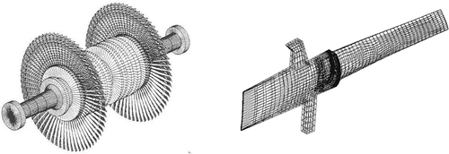
The mechanical model of the bladed disk developed here is a finite element model (Figure 2). The outputs of interest of the model are the resonance frequencies and vibration amplitudes of each blade. The dynamic sub-structuring technique reduces the required level of computational effort 34, but reliable predictions remain expensive. Indeed, as mistuning destroys the cyclic symmetry of the bladed disk assembly, one needs several Monte Carlo simulations of the finite element models to reproduce vibration statistics.

Figure 2. Left: bladed disk, right: disk sector and blade mesh (11437 nodes).

5.2. Parametrization of the probabilistic uncertainty model

Mistuned bladed disks are classically modelled through perturbations of the Young's modulus of individual blades, which leads to fixed mode-shape changes. In contrast, the preferred approach is to directly construct a probabilistic model of the stiffness matrix of each sub-structure (blades and disk). Such an approach has been proposed in 35 for general structures and in 36 for structures with cyclic symmetry. First, it enables a realistic representation of the mode-shape changes when the variations in stiffness matrices are large: and second, as already mentioned in Section 4.2, it replaces the direct construction of the probabilistic model of all the individual input parameters by a parsimonious parameterization.

In order to account for the observed mode-shape variability, a large number of inputs of the finite-element model (such as elementary Young modulus, component dimensions, etc.) may be modelled as random. In particular, the ν x ν reduced stiffness matrix K_ν of the substructures of the model corresponding to each blades 35 comprises more than 20,000 elementary input variables in the present case. The parsimonious parameterization of such an uncertain matrix consists in describing it by the lowest number of parameters upon the constraint of the true information available. As a natural mechanical property, this matrix is supposed to belong to an ensemble of positive-definite symmetric real-valued random matrices. Beyond that, what can be directly inferred on the detail pdf of each of 20,000 uncertain inputs that constitute the matrix is not much: a best-estimate value and the existence of a non-negligible dispersion. In this context, the minimal parameterization includes simply a mean (positive-definite) value E[K_ν] and a single global dispersion parameter δ to be calibrated against indirect data (blade resonance frequencies, cf Section 5.3). Hence, 28 identifies the type of distribution that ought to be used in such a case, through a generalization of the principle of maximal entropy. A classical application of this principle states that a random variable, a priori unbounded, and parameterized simply by mean and dispersion should be Gaussian. A matrix generalization proves that the joint pdf of such random matrices should be modelled by a dedicated family of matrix distributions determined by E[K_ν] and a dispersion parameter δ which summarizes the variance of the matrix. For algebraic consistency, such a variance has to be normalized over the space of definite-positive matrices as follows: (27) where (28) Note in particular that a deterministic matrix where dispersion around E[K_ν] is negligible implies δ = 0. Hence, the probabilistic model of input uncertainty is: where f_K denotes a known joint pdf for the matrix coefficients, for which a closed-form (though complicated) expression may be found in 28, along with the Monte Carlo simulation details.

Figure 3 illustrates the impact of such a parameter upon the probabilistic distribution of the magnification factor of vibration amplitude. The quantiles of this magnification factor have been computed from the previously-described probabilistic and mechanical model for different values of the parameter δ. The parameter δ appears as the mistuning driver: in the absence of dispersion (δ = 0), amplitudes of the various blades are comparable and all vibrate at a homogeneous frequency. When δ increases, blade resonance frequencies get dissimilar and magnification increases significantly. Beyond a certain critical value, the magnification factor drops.

Figure 3. Percentiles of the vibration amplitude magnification factor vs. the dispersion parameter δ.

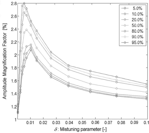
Consequently, tolerance relaxation or intentional detuning could increase maximum vibrations if the initial value of δ is smaller than the critical value or decrease them otherwise. This highlights the relevance of identifying properly the δ parameter in order to know how design modifications could affect the level of amplitude magnification.

5.3. Data from in situ real-bladed disks and the inverse problem

The best-estimate finite-element model of each structural element is classically estimated separately by mechanical expertize, standard design parameters and modellers’ expertize, so that the expectation E [K_ν] is considered to be well known. In particular, sub-structures mechanical model can be identified from individual measurements on removed blades or disk, i.e. outside normal operating conditions. This classical identification step is not recalled in this article as the focus is placed onto the estimation of the one-dimensional dispersion parameter θ_X = δ which proves much more challenging. Indeed, because of the large variety of possible mistuning sources and sensitivity of the mistuning phenomenon to small perturbations, the dispersion parameter δ should only be identified according to non-intrusive measurement of real-bladed disks operating under normal conditions. Because of the inter-blades coupling effect, measurement of individual removed blades are irrelevant to identify δ.

Measurements of vibrations in rotating bladed assemblies are undertaken with a blade tip timing technique 37. The studied bladed disk has 77 blades. The 77 lowest resonance frequencies ()_l=1…77 are measured on n = 3 distinct bladed disks. As a plausible metrological statement, the measurement error is supposed to be Gaussian with a null mean value and a standard deviation corresponding to one-tenth of the total dispersion of resonance frequencies, i.e. of the empiric standard deviation of all 3 × 77 frequency observations mixed together. In addition, the theoretically-identical bladed disks are assumed to be identically distributed with the same E [K_ν] and δ. This means that the three-bladed disks correspond to three independent realizations of K_ν. Additionally, they operate under equivalent operational conditions d representing power, void conditions, etc. Hence, the data sample is constituted by 3 i.i.d. realizations of vectors y_m of dimension 77 with a fixed value of vector d: (29) The probabilistic model is that of (8) and does evidence a highly non-linear behaviour of H with respect to x (30) An important comment regards the information content and size of the sample Ξ_n. Measuring three-bladed disks under normal operation represents already quite a large operational cost and should be seen as a lucky amount of data at hand in a such an application. Yet, taken at ‘face value’, a three-sample could be seen as a very low-sized-sample for the implementation of asymptotically-converging algorithms. As a matter of fact, the physically-relevant information content of the sample is closer to n × m = 3 × 77 than to 3. Indeed, the mistuning phenomenon randomly disturbs the 77 blades of each bladed disk, each blade expressing different physical DOF of the system, all parameterized by a single common parameter δ to be estimated. If those blades were fully independent from each other, the equivalent sample size should be 3 × 77 from an estimation point of view. In fact, each blade frequency is a distinct deterministic function of the same random stiffness matrix K_ν which itself gathers a large number (over a thousand) of independent elementary random DOF: while it is not possible to guarantee independence because of complex deterministic cross-coupling of those elementary DOF, it is physically sound to assume that the 77 blades represent a large number of independent DOF.

Note that a finer uncertainty model parameterization could theoretically replace the single parameter θ_X = δ by a vector of parameters. Such a vector could include for instance: a parameter representing the mass dispersion within the mass reduced matrices that is not modelled so far; more parameters distinguishing stiffness or mass dispersion per substructures. Yet, additional experimental information would be necessary for this new set to be properly identified and this is likely to exceed the industrially-reasonable data basis.

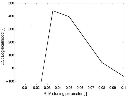
5.4. Results of the simulated likelihood algorithm

The complete log-likelihood (15) is computed according to the algorithm described in Section 4. Figure 4 shows the result as a function of δ with the following values: n = 3 blades observed, n_s = 50 mechanical computations to simulate the model likelihood (because d is fixed, the reproduction of n times those n_s computations is unnecessary), and N_r = 5000 error noise simulations. The maximal likelihood is reached for : because of the associated computational costs, the discretization of δ has been kept at a rather coarse level, which may appear insufficient at first hand. Yet, a very rough accuracy of ±0.01 may be graphically inferred in Figure 4 from the curvature of the identification curve, remembering that the asymptotic variance of a MLE is classically known to be the inverse of the information matrix or local curvature of the log-likelihood: (31) Such accuracy is quite sufficient for the industrial needs, and turns out to be of the same order of magnitude as the remaining (non-modelled) epistemic uncertainties (cf Section 0). With a dispersion of δ= 0.035, the vibration level is amplified by a factor between 1.6 and 1.9 (0.05/0.95-percentiles), which is physically sound.

Figure 4. Complete log-likelihood as a function of δ, for n × m = 3 × 77, n_s = 50, N_r = 5000.

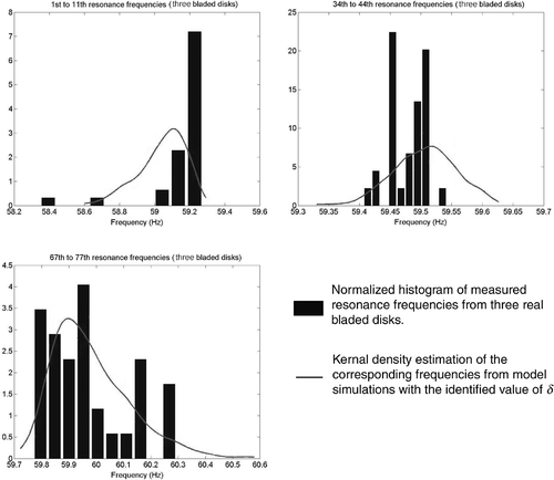
Once the uncertainty model has been identified by the choice of such a MLE for δ, simulations of the probabilistic mechanical model can be compared to on-site frequency measurements. The 77 observed resonance frequencies of each of the three-bladed disks are grouped within seven subsets by increasing values. This is meant to construct histograms with large-enough number of values for them to be comparable to simulated distributions. Each subset contains 11 × 3 resonance frequencies: this means that histograms are only approximate as they mix the distributions of 11 distinct blades which are closely but not truly identically-distributed. Yet, these subsets are simply used for the a posteriori graphical comparison, and were not involved in the identification process. Figure 5 compares then the simulated densities (taking the identified value δ = 0.035) to the measured sample of resonance frequencies. Goodness of fit is deemed acceptable since the essential feature is the average dispersion of frequencies: indeed, distribution tails referring to the frequency deviation of individual blades are less relevant to the magnification factor.

Figure 5. Measured and simulated resonance frequencies densities for three sets of 77 resonance frequencies.

6. Conclusion and further research needs

Full probabilistic inversion is intended to supply information on the distribution of intrinsic (or irreducible, aleatory) input uncertainty. After clarifying the differences with classical data assimilation or parameter identification techniques, this article has introduced a new non-parametric algorithm that does not require the linear and Gaussian assumptions of existing ones. It was implemented within an industrial study of turbine vibration within which the intrinsic variability linked to design or manufacturing imperfections is the key factor generating a potential increase of fatigue. Experimental observations of resonance frequencies enabled the calibration of a single global dispersion parameter and hence model satisfactorily the variability controlling the subsequent probabilistic risk assessments.

Beyond this first industrial example needing deeper benchmark against alternative algorithms, the algorithm could obviously be applied to other models with an increasing dimension for θ_X that should challenge its computing cost to convergence. More generally, further research is required regarding: (a) a comprehensive convergence study according to the size of the data sample, with implications on the choice of the optimal smoothing of the simulated likelihood; (b) the optimization of the compromise robustness/CPU cost in the case of larger dimensions for X or large CPU-consuming physical models: this raises the question of choosing an efficient multi-dimensional optimization algorithm within the iterative process, for instance through EM-inspired algorithms; (c) the integration of expert under Bayesian extensions, whereby physical considerations could supplement the relative scarcity of data.

To cover a larger range of situations regarding physical model regularity and input–output dimensions, other algorithms could obviously complement the one proposed in this article, including: adaptive linearization of the physical model within the likelihood maximization process; a mixture of MM and later local likelihood maximization to optimize the number of model runs; adaptive response surfaces approximating the physical model itself, while relying on an ‘exact’ likelihood maximization process, etc.

More fundamentally, the authors stress the interest of a deeper debate about the pros and cons of classical data assimilation or parameter identification formulations versus intrinsic variability formulations such as that of the present article. As discussed in the general uncertainty literature in relation with epistemological and applied decision-theory considerations, practical modelling choices on the nature of physical uncertainty and variability are needed within inverse probabilistic approaches, with essential statistical and numerical consequences.

Acknowledgements

We thank Louis Ratier, Philippe Voinis and Loic Berthe for their contribution to Section 5. We thank Yannick Lefebvre (EDF R&D) as well as Paul Mahé for their fruitful contribution in the generation of the ideas of this article.

Notes

Note

1. Note that data assimilation techniques are less used in this simple static formulation than in dynamic cases, whereby (Y_j, d_j) are time series, and x refers to initial conditions: that dynamic setting is not the object of the present article.

References

- Parry, GW, and Winter, PW, 1981. Characterization and evaluation of uncertainty in probabilistic risk analysis, Nucl. Safety 22 (1981), pp. 28–42.
- Beck, MB, 1987. Water quality modelling: A review of the analysis of uncertainty, Wat. Res. 23 (1987), pp. 1393–1442.
- Apostolakis, G, 1990. The concept of probability in safety assessments of technological systems, Science 250 (1990), pp. 1359–1364.
- Granger Morgan, M, and Henrion, M, 1990. Uncertainty–A Guide to Dealing with Uncertainty in Quantitative Risk and Policy Analysis. London: Cambridge University Press; 1990.
- Helton, JC, and Burmaster, DE, 1996. Guest editorial: Treatment of aleatory and epistemic uncertainty in performance assessments for complex systems, Rel. Eng. Syst. Saf. 54 (1996), pp. 91–94.
- Beck, JV, and Arnold, KJ, 1977. Parameter Estimation in Engineering and Science. New York: Wiley; 1977.
- Tarantola, A, 2004. Tarantola, A, ed. Inverse problem theory and methods for data fitting and model parameter estimation. Amsterdam: SIAM, Elsevier; 2004, 1987.
- Talagrand, O, and Courtier, P, 1987. Variational assimilation of meteorological observations with the adjoint vorticity equation, I: Theory, Q. J. R. Meteorol. Soc. 113 (1987), pp. 1311–1328.
- Helton, J, 1993. Uncertainty and sensitivity analysis techniques for use in performance assessment for radioactive waste disposal, Rel. Eng. Syst. Saf. 42 (1993), pp. 327–367.
- Paté-Cornell, ME, 1996. Uncertainties in risk analysis: Six levels of treatment, Reliab. Eng. Syst. Saf. 54 (1996), pp. 95–111.
- Helton, JC, and Oberkampf, WL, 2004. Alternative representations of epistemic uncertainty, Rel. Eng. Syst. Saf. 85 (1–3) (2004), pp. 1–369.
- Talagrand, O, 1997. Assimilation of observations, an introduction, J. Meteor. Soc. Japan 75 (1997), pp. 191–201.
- Walter, E, and Pronzato, L, 1994. Identification de Modèles Paramétriques à partir de données expérimentales. Masson: Coll. MASC; 1994.
- Beck, JL, and Katafygiotis, LS, 1998. Updating models and their uncertainties, J. Eng. Mech. I: Bayesian Statistical Framework 124 (1998), pp. 455–461.
- Casarotti, C, Petrini, L, and Strobbia, C, 2007. "Calibration of non-linear model parameters via inversion of experimental data and propagation of uncertainties in seismic fibre element analysis". In: Proceedings of Computational Methods in Structural Dynamics and Earthquake Engineering, Rethymno. 2007.
- Mahé, P, and Rocquigny, E de, 2005. Incertitudes non observables en calcul scientifique industriel–Etude d’algorithmes simples pour intégrer dispersion intrinsèque et ébauche d’expert, 37èmes J. Franc. Stat. Pau (2005), France.
- Du, C, Kurowicka, D, and Cooke, RM, 2006. Techniques for generic probabalistic inversion, Computational Statistics & Data Analysis 50 (5) (2006), pp. 1164–1187.
- De Crécy, A, 1997. CIRCE: A tool for calculating the uncertainties of the constitutive relationships of Cathare2, in 8th International Topical Meeting on Nuclear reactor Thermo-Hydraulics (NURETH8). Kyoto. 1997.
- Dempster, F, Laird, NM, and Rubin, DB, 1977. Maximum likelihood from incomplete data from the EM algorithm, J. Roy. Stat. Soc. (Ser. B) 39 (1977), pp. 1–38.
- de Rocquigny, E, 2006. La maîtrise des incertitudes dans un contexte industriel: 1ère partie–Une approche méthodologique globale basée sur des exemples; 2nd partie–Revue des méthodes de modélisation statistique, physique et numérique, J. Soc. Française Stat. 147 (2006), pp. 33–106.
- Rocquigny, E de, Devictor, N, and Tarantola, S, 2008. Uncertainty in Industrial Practice, A Guide To Quantitative Uncertainty Management. Chichester: Wiley; 2008.
- Ionescu-Bujor, M, and Cacuci, DG, 2004. A comparative review of sensitivity and uncertainty analysis of large-scale systems–I: Deterministic methods, Nucl. Sci. Eng. 147 (2004), pp. 189–2003.
- Cacuci, DG, and Ionescu-Bujor, M, 2004. A comparative review of sensitivity and uncertainty analysis of large-scale systems–II: Statistical methods, Nucl. Sci. Eng. 147 (2004), pp. 204–217.
- Hamby, DM, 1994. A review of techniques for parameter sensitivity analysis of environmental models, Environ. Monit. Assess. 32 (1994), pp. 135–154.
- Frey, HC, and Patil, SR, 2002. Identification and review of sensitivity analysis methods, Risk Anal. 22 (2002), pp. 553–578.
- Saltelli, A, Tarantola, S, Campolongo, F, and Ratto, M, 2004. Sensitivity Analysis in Practice: A Guide to Assessing Scientific Models. Chichester: John Wiley and Sons; 2004.
- Helton, JC, Johnson, JD, Sallaberry, CJ, and Storlie, CB, 2006. Survey of sampling-based methods for uncertainty and sensitivity analysis, Reliab. Eng. Syst. Saf. 91 (2006), pp. 1175–1209.
- Soize, C, 2005. Random matrix theory for modelling uncertainties in computational mechanics, Comput. Methods Appl. Mech. Eng. 194 (2005), pp. 1333–1366.
- Silverman, BW, 1986. Density Estimation for Statistics and Data Analysis. London: Chapman and Hall; 1986.
- Rubinstein, RY, 1981. Simulation and the Monte-Carlo method. New York: Wiley; 1981.
- Cramér, H, 1946. Mathematical Methods of Statistics. Princeton, NJ: Princeton University Press; 1946.
- Jennrich, RI, 1969. Asymptotic properties of non-linear least squares estimators, Ann. Math. Statist. 40 (1969), pp. 633–643.
- Hoadley, B, 1971. Asymptotic properties of maximum likelihood estimators for the independent not identically distributed case, Ann. Math. Statist. 42 (1971), pp. 1977–1991.
- Ratier, L, 2004. "Modelling a mistuned bladed disk by modal reduction". In: Proceedings of ISMA2004, Leuven 2004. 2004.
- Soize, C, 2000. A non-parametric model of random uncertainties for reduced matrix models in structural dynamics, Probab. Eng. Mech. 15 (2000), pp. 277–294.
- Capiez-Lernout, E, and Soize, C, 2004. Nonparametric modeling of random uncertainties for dynamic response of mistuned bladed disks, J. Eng. Gas Turbine Power 126 (2004), pp. 610–618.
- Ratier, L, and Voinis, Ph.S, 2002. "Study of blade dynamic stresses with a non intrusive measurement technique: Experimental results on a power station turbine". In: Proceedings of 9th ISROMAC. Honolulu, 2002 February 10–14. 2002.