Reconstruction of part of a boundary for the Laplace equation by using a regularized method of fundamental solutions

Abstract

In this article, the identification of part of a boundary for the two-dimensional Laplace equation is investigated. One regularized method of fundamental solutions is used for determining an unknown portion of the boundary from the Cauchy data specified on a part of the boundary. Since the resulting matrix equation is badly ill-conditioned, a regularized solution is obtained by employing the Tikhonov regularization technique, while the regularization parameter for the regularization method is provided by the generalized cross-validation criterion. The numerical results show that the proposed method produces a convergent and stable solution.

Keywords:

• Laplace equation
• the method of fundamental solutions
• Tikhonov regularization
• inverse boundary problem

1. Introduction

The non-destructive evaluation of a corrosion boundary attracts more and more interest in engineering and mathematics. Unfortunately, in many practical situations, the known boundary data are not complete, and corrosion takes place on an inaccessible part of the boundary. Our task is to determine the shape of a corrosive boundary from the measured data. This is an inverse boundary problem, and it is extremely ill-posed, namely a small perturbation in the measured data may cause a dramatically large error for the solution 1.

The inverse boundary problems recently received many mathematical studies, and both stability and identifiability issues have been investigated. The proof on the uniqueness and stability of the solution was given by Bukhgeim et al. 2, in which a very weak conditional stability estimate of logarithmic rate was given under a regularity assumption on the unknown boundary, and then the theoretical result was extended to ℝ³ 3. Stability of various forms has also been extensively studied in 4,5.

Several numerical methods have been proposed for the inverse boundary determination problems. Mclver 6 and Michael et al. 7 devised a non-destructive evaluation technique by applying an alternating current to the accessible boundary and determined the corroded boundary by observing the output current fields. Charton et al. 8 proposed a variational technique based on parameterizing the unknown boundary using the function specification method. Nachaoui 9 applied a conjugate gradient method to identify the corroded boundary, and the boundary element method (BEM) was employed to discretize the intermediate direct problems. The numerical scheme based on the BEM in conjunction with the Tikhonov first-order regularization procedure has been studied by Lesnic et al. 10,11. In 12, Hon and Wu developed a meshless method based on radial basis interpolation to determine an unknown boundary where they provided a good approximation of the solution with exact data. However, the numerical results are unstable while using noisy data due to the bad conditioning of the interpolation matrix. Recently, Liu et al. 13 have used the Fourier expansion technique with the Lavrentiev regularization to solve the inverse geometry heat conduction problem in a two-dimensional rectangle.

In recent years, meshless methods have attracted great attention in the scientific and engineering community. Meshless methods emerge as a competitive alternative to mesh-dependent methods, including the radial basis functions (RBF) method 14,15, the method of fundamental solutions (MFS) 16,17 and the boundary knot method (BKM) 18,19. These meshless methods require neither domain discretization as in the finite element method (FEM) and finite different method (FDM) nor boundary discretization in the BEM, thus they improve computational efficiency and can be easily extended to solve high-order and high-dimensional differential equations. In this article, we propose a non-iterative numerical method based on the MFS combined with the Tikhonov regularization (TR) technique to solve the inverse boundary problem by using the noisy data. More recently, Hon and Li 20 employed the MFS to solve an inverse boundary determination problem for heat equation. Mera et al. 21,22 used a variational technique to identify the unknown boundary for the Laplace equation in which the MFS is used to solve a direct problem. Nevertheless, we have not seen similar papers which use the MFS to reconstruct part of a boundary for the Laplace equation.

The article is organized as follows. In Section 2, we formulate the problem mathematically. The MFS is described in Section 3. The regularization technique and the rule for choosing a regularization parameter are presented in Section 4. In Section 5, we show the results for several numerical examples. Section 6 provides a summary and concluding remarks.

2. Mathematical formulation of the problem

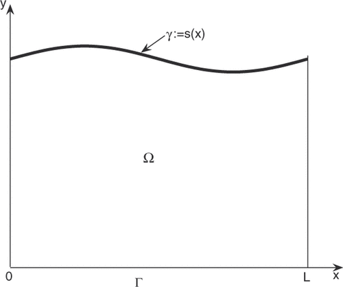
In this article, the MFS is used to determine material loss occurring on the inaccessible boundary γ ⊂ ∂ Ω with the domain Ω ⊂ ℝ² by measuring Cauchy data on an accessible portion of the boundary. Therefore, we consider the following boundary identification problem: (1) (2) (3) where L represents a linear elliptic partial differential operator, Γ is the accessible part of the boundary ∂Ω with given function values f and g and ν is the outward normal to the boundary Γ. It is not required that Γ ∪ γ = ∂ Ω. The problem is then to determine the shape of the unknown boundary γ from the Cauchy data f, g.

For numerical verification, we focus on solving the following 2D Laplace equation in the domain Ω, described in Figure 1, referring to 12,23 (4) subject to the boundary conditions (5) (6) where Δ is the Laplacian operator and u₀ is a constant.

Figure 1. The solution domain of the boundary identification problem.

It should be mentioned that the formulation of the problem can be associated with other elliptic partial differential equations, such as the Helmholtz equation (see 24, and references therein). Other domains, smooth or non-smooth, can be investigated by the same method but are not considered in this article. This is an ill-posed problem and thus it is impossible to solve using classical numerical methods, and special techniques should be employed.

3. The method of fundamental solutions

Since all the quantities involved are on the boundary, the use of the boundary-type technique for the solution of partial differential equations seems natural. The BEM reduces the dimensionality of the problem by one, thus it partly alleviates the difficulty. However, it requires the evaluation of singular integrals for using singular fundamental solutions and requires the meshing of the boundary, which can be difficult for complicated geometries in high dimensions. The MFS avoids the difficulties. It is a boundary-type meshfree technique for the solution of partial differential equations and it has become very popular in recent years due to its ease of implementation. The basic idea of the MFS is to approximate the solution of the governing partial differential equation by a linear combination of fundamental solutions with singularities located on a fictitious boundary outside the solution domain. It should be noted that the MFS in conjunction with regularization methods has successfully been applied to inverse problems, such as the Cauchy problem for various partial differential equations 25–27 and inverse heat conduction problems 28,29. In 27, the authors compared the effects of several regularization techniques and found that the TR with a generalized cross-validation choice of the regularization parameter is more effective while using the MFS. Motivated by the encouraging numerical results reported in these works, we use the MFS for solving an inverse boundary determination problem in the current investigation. The numerical results show the MFS method is effective. To achieve the same accuracy as FEM or BEM, the corresponding mesh used must be very fine, which undoubtedly would increase the computational time considerably. So our method is suitable for solving the inverse problem.

The fundamental solution for the Laplacian operator Δ is given by 30: (7) where P, Q are points in ℝ² with |P − Q| denoting their Euclidean distance in ℝ². When the source point Q is located outside the domain , the fundamental solution satisfies the Laplace equation in domain Ω.

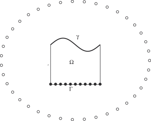
On the boundary Γ, we choose n collocation points . A total number of l source points are then placed at the fictitious boundary outside the solution domain as shown in Figure 2.

Figure 2. The boundary identification problem for solution domains Ω. Dots (•) are collocation point for boundary data. Circles (○) represent source points.

In the MFS, the solution of the problem (2.4–2.6(4) ) is approximated by a linear combination of the fundamental solutions, namely (8) where are unknown coefficients to be determined.

Generally, there are two approaches to choose : fixed and adaptive schemes. Since the fixed scheme is adopted in this article for simplicity, readers may refer to the work of Fairweather and Karageorghis 17 on the adaptive scheme. In the fixed scheme, the points are chosen a priori in a certain fixed setting. In this article the source points are uniformly distributed on a circle with radius r, see Figure 2 for the configuration.

The approximate solution satisfies the governing differential equation, and the coefficients are chosen to satisfy the boundary conditions. By collocating the boundary conditions at {P_i}, it is easy to get the following system of linear equations: (9) (10)

In brevity, we obtain the following matrix equation: (11) where A = (A_ij) is an interpolation matrix, d = (λ₁, …, λ_l) is a coefficient vector to be determined and b is the known data vector.

It should be noted that in order to uniquely determine the solution of the system of linear algebraic equation (3.5(11) ), the number n of boundary collocation points and the number l of source points must satisfy the inequality l ≤ 2n.

The matrix equation arising from the MFS is often severely ill-conditioned, and measured data for inverse problems are usually noisy. Thus we must take special care when solving them.

4. Regularization method

The main difficulty of the MFS is that the interpolation matrix A may be highly ill-conditioned. For the solution of forward problems with exact data, this does not pose great challenges, since no noise is considered in the data. Standard methods may be able to yield accurate results. However, for inverse problem, the situation is delicate. Inverse problems are usually ill-posed, and the ill-conditioning is caused by the discrete formulations. Most of numerical methods for treating discrete ill-posed problems seek to overcome the conditioning by replacing the resulting matrix with a well-conditioned matrix whose solution approximates the required solution. The regularization technique usually gives a better control on the level of numerical accuracy to the original problem but requires a good choice of regularization parameter for optimal performance. During the last decades, some regularization methods for treating discrete ill-posed problems have been successfully developed 31. However, we only consider the TR method 32 in our study. All the computational codes are written in MATLAB, and in particular the MATLAB code developed by Hansen 33 is based on singular value decomposition (SVD), which has been adopted in our computations, to solve the discrete ill-posed problem (3.5(11) ).

In the SVD, the matrix A is decomposed into (12) where and are column orthonormal matrices, with column vectors called left- and right-singular vectors, respectively. The superscript * denotes matrix transposition. The matrix has non-negative diagonal elements in decreasing order, which are the singular values of A. On the basis of SVD, the least-squares (LS) solution d^o of the matrix equation (3.5(11) ) has the formula (13) where k is the rank of the matrix A. For the ill-conditioned matrix equation, there are small singular values, therefore the LS solution is dominated by contributions from small singular values when noise is existed in the data, we need to use regularization methods to filter the errors corresponding to these small singular values. In this study, we use the TR method.

The Tikhonov regularized solution d_α for problem (3.5(11) ) is defined as the solution to the following LS problem: (14) where ∥ · ∥ is the Euclidean norm and α is a regularization parameter.

Formally, the Tikhonov regularized solution d_α of the problem (4.3(11) ) is then given as the solution of the following regularized equation: (15) where I is the unit matrix.

The choice of a suitable value of the regularization parameter α is crucial for the accuracy of the final numerical solution and is still under intensive research 35. In this article we use the generalized cross-validation (GCV) criterion to choose a good regularization parameter, which is to minimize the following GCV function 35: (16) where A^I is a matrix that produces the regularized solution when multiplied with b, i.e. d_α = A^Ib.

Denote the regularization parameter given by GCV rule as and the corresponding regularized solution by then the approximate solution can be written as (17)

Let (18) we can solve equation (4.7(18) ) for the unknown boundary This gives the approximation for the unknown boundary

5. Numerical verification

In this section, we present the numerical results by the proposed numerical scheme to verify its efficiency. The convergence and the stability of the method with respect to the distance between the source points and the boundary of the solution domain and decreasing the amount of noise added into the input data are carefully investigated.

In many practical situations, the measured data are unavoidably contaminated by inherent measurement errors. Thus, in this section we replace the exact data with noisy data as follows: (19) (20) where f_i : = f (P_i), g_i : = g(P_i), ε indicates the percentage relative noise error and the rand(i ) is a random number chosen in [−1, 1].

In order to measure the accuracy of a numerical solution, we define the relative root mean square error as (21) where N is the total number of testing points on γ, s_i and are the exact and approximated value at these points, respectively. In our computations, we always take N = 21.

5.1. Numerical examples

For the convenience to illustrate the accuracy of the method, let Ω = {(x, y) : 0 ≤ x ≤ 10, 0 ≤ y ≤ s(x)}, Γ = {(x, y) : 0 ≤ x ≤ 10, y = 0}, we consider the following examples:

Example 1

The analytical solution u(x, y) is taken to be (22) Let u₀ = 160, then we obtain the corresponding corrosion boundary s(x) from the following equation: (23)

Example 2

The analytical solution u(x, y) is taken to be (24)

Let u₀ = 1, the corresponding corrosion boundary is γ : s(x) = 1.

Example 3

The analytical solution u(x, y) is taken to be (25)

Let u₀ = 31, the corresponding corrosion boundary is γ : s(x) = 4.

The boundary data f and g are obtained from the given exact solutions.

Example 4

We consider an example where there is no analytical solution to the problem. (26) (27) (28) (29) (30) and the corresponding continuous corrosion boundary is (31)

Example 5

In this example, the corresponding discontinuous corrosion boundary is (32)

For Examples 4 and 5, the value of u(x, 0) = f (x) is obtained from solving the problems (2.4–2.6(4) ) by using the collocation method given in 13.

Unless otherwise specified, the fictitious boundary is a circle centred at (5, 0) with radius 8 for the domain Ω. In our computations, we take l = 21 source points uniformly distributed on the fictitious boundary. Furthermore, the number of boundary collocation points is n = 21.

5.2. Effect of regularization

In this subsection, we investigate how the regularization method improves the accuracy of numerical results for noisy data. We consider Example 1 with noise of ε = 1% in the data.

For noisy data, standard methods for solving matrix equation (3.5(11) ), such as the LS method, cannot yield a stable result. The unknown boundary γ by the LS method is displayed in Figure 3(a). From the figure, it is easily seen that the LS method gives an unstable solution to the problem, and it is highly oscillatory. As explained in Section 4, the large oscillations in the solution are due to the contributions from the small singular values and the presence of noise in the data. The condition number is approximately 6.6 × 10⁶, which is enormous compared with the size of the interpolation matrix A. The corresponding GCV analysis for the problem is shown in Figure 3(b). From this figure, the regularization parameter is found to be 0.015821. We note that similar results are obtained when using other non-regularization methods to solve the resulting matrix equation, although they are not presented here.

Figure 3. (a) Numerical solutions of the unknown boundary s(x) for Example 1 with 1% noise added into the data; (b) the corresponding GCV function.

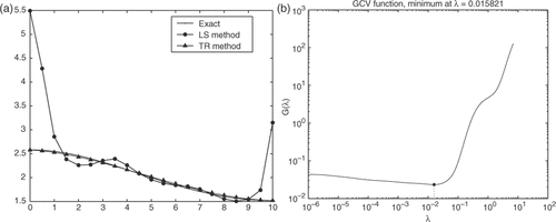
The numerical solutions obtained by using the TR method are also shown in Figure 3(a), where the regularization parameter is chosen by GCV rule. Compared with the results by the LS method, the numerical solution by the TR method is an excellent agreement with the analytical solution. Therefore the regularization method is indispensable to obtain stable and accurate results in the case of noisy data. The results also show that the GCV method provides an effective regularization parameter for the TR method.

5.3. Analysis of numerical results

In this subsection, we present the numerical results for the Examples 1–5 by using both exact and noisy data.

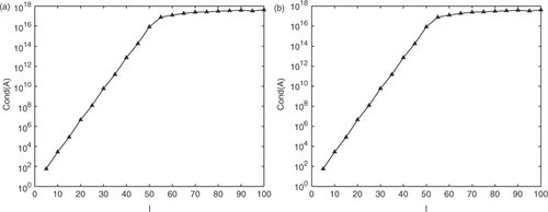
Figure 4 shows the condition number of the matrix A with n = l. It can be seen that the condition number Cond(A) increases exponentially up to l = 60 for Examples 1 and 2. Therefore, the problem is severely ill-posed.

Figure 4. The condition number, Cond(A), as a function of the number of source points l with n = l (a) for Example 1; (b) for Example 2.

Our first example is taken from 13. In 13, this problem was solved by the Laventiev regularization, however, they only consider the noise-free data. Here we solve this problem by MFS + TR. The numerical results for Example 1 with various levels of noise in the data are shown in Figure 5(a). The corresponding regularization parameters given by GCV criterion are presented in Table 1. From Figure 5(a) and Table 1, we can see with up to 3% noise in the data, the numerical solution is still in good agreement with the analytical solution. Similar results can be obtained for Example 2, which are shown in Figure 5(b) and Table 2.

Figure 5. The exact solution and its approximation with various levels of noise added into the measured data. (a) Example 1; (b) Example 2.

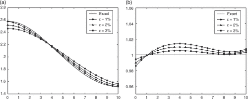
Table 1. The regularization parameters and the rel with various levels of noise added into the data for Example 1.

	1%	2%	3%
	0.0158	0.0250	0.0352
rel	0.0096	0.0229	0.0389

Table 2. The regularization parameters and the rel with various levels of noise added into the data for Example 2.

	1%	2%	3%
	0.0072	0.0103	0.0127
rel	0.0035	0.0066	0.0096

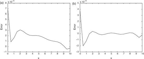
The MFS can be extremely accurate for exact data. Consider Example 1 with exact data, and the error distribution for the numerical results is illustrated in Figure 6. The maximum error for the numerical results retrieved by the LS is 1.1 × 10⁻⁴, while its corresponding value obtained by using the TR is 4.8 × 10⁻⁵, which clearly show that our method also produces comparable accuracy as 13.

Figure 6. The error between the exact solution and its numerical solution with the exact Cauchy data for Example 1. (a) LS method; (b) TR method.

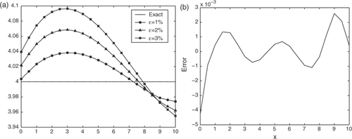
The results for Example 3, obtained by using various levels of noise added into the data, are illustrated in 7. It can be seen from Figure 7(a) that the numerical results retrieved for the part of boundary represent good approximations for their analytical values. By comparing the results of Example 2 (e.g. Figure 5(b)), we find that the closer the distance from the unknown boundary to the boundary where the collocation points are located, the better the accuracy in the numerical result.

Figure 7. (a) The exact solution and its approximation with various levels of noise added into the measured data; (b) the error between the exact solution and its numerical solution by noise-free data for Example 3.

In order to investigate the stability of the MFS, we set the relative noise level ε = [10⁻⁵–10⁰, 2, 3, 5, 10]%. The numerical results are graphically reported in Figure 8(a) for Example 2. It can be observed that the numerical solution is convergent nicely with respect to the decreasing value of the relative noise levels.

Figure 8. Relative error for TR+GCV with (a) various levels of noise, ε; (b) various radius of source points, r.

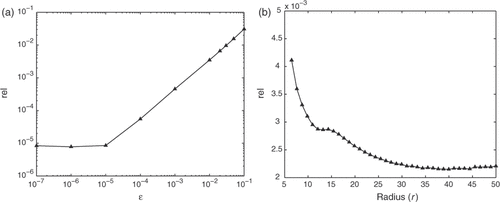
Next, we study the stability of the numerical solutions with respect to the radii r of the circle on which the source points are distributed for Example 2. In Figure 8(b), we present the relative errors rel as a function of r, obtained by using with a fixed relative noise level ε = 1%. From this figure, it can be seen that the larger r is, the better the accuracy in the numerical results. We note that the value r = 20 is sufficiently large such that any further increase in the radius r do not significantly improve the accuracy of the numerical results.

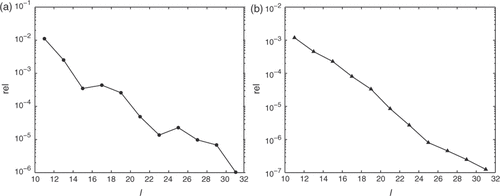
Further, we investigate the sensitivity of the scheme with respect to increasing the number of collocation points and source points. For simplicity, the numerical results are presented in Figure 9 with l = n and the exact data. These results indicate that the MFS in conjunction with the TR + GCV method provides accurate numerical results with respect to the increase in the number of collocation points and source points. Thus a few collocation points are sufficient to yield very accurate results, and the size of the resulting matrix equation is quite small, therefore the proposed method is efficient.

Figure 9. Relative error rel for TR + GCV obtained by using exact data, as a function of the number of source points l with n = l (a) for Example 1; (b) for Example 2.

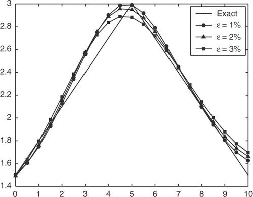
We have investigated the performance of the method for problems with an analytical solution. In fact, the method works equally well for the examples without analytical solutions. To illustrate this point, we consider Examples 4 and 5. In Example 4, the corrosion boundary is a continuous piecewise smooth function. The analytical formula to the temperature f (x) is not available, and thus the numerical solution to the forward problem is solved as the exact data. The numerical results for Example 4, which were obtained with various levels of noise added into the data are presented in Figure 10. From this figure, as well as Table 3, even for a relatively high amount (ε = 3%) of noise added into the data, the numerical results retrieved for the corrosion boundary represent good approximations of the exact values.

Figure 10. The exact solution and its approximation for Example 4 with various levels of noise added into the measured data.

The numerical results for Example 5 in which the corrosion boundary is a discontinuous function are presented in Figure 11. From this figure and Table 4, we can see that the numerical results are less accurate than the other examples and the MFS cannot identify a discontinuous boundary by our judgement. The total-variation regularization 36 may be employed to circumvent the undesirable smoothing effect.

Figure 11. The exact solution and its approximation for Example 5 with various levels of noise added into the measured data.

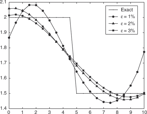
Table 3. The regularization parameters and the rel with various levels of noise added into the data for Example 4.

	1%	2%	3%
	0.0025	0.0040	0.0059
rel	0.0410	0.0418	0.0425

Table 4. The regularization parameters and the rel with various levels of noise added into the data for Example 5.

	1%	2%	3%
	0.0014	0.0174	0.0243
rel	0.0569	0.0599	0.0605

6. Conclusions

In this article, we study a meshless method for solving an identification of a corrosion boundary problem. The problem is solved by using the MFS. The resulting system of linear algebraic equations is ill-conditioned and therefore its solution is regularized by employing the TR method, while the choice of the regularization parameter is based on GCV criterion. The numerical results indicate that the proposed scheme is effective and stable for reconstructing an unknown boundary.

Acknowledgements

The authors would like to thank the referees for their careful reading and valuable suggestions that improve the quality of our article. The work described in this article was supported by the NSF of China (10571079, 10671085) and the program of NCET.

References

- Hadamard, J, 1923. Lectures on Cauchy's Problem in Linear Partial Differential Equations. London: Oxford University; 1923.
- Bukhgeim, AL, Cheng, J, and Yamamoto, M, 1998. "Uniqueness and stability for an inverse problem of determining a part of boundary". In: Inverse Problems in Engineering Mechanics (Nagano, 1998). Oxford: Elsevier; 1998. pp. 327–336.
- Cheng, J, Hon, YC, and Yamamoto, M, 2001. Conditional stability estimation for an inverse boundary problem with non-smooth boundary in R3, Trans. Amer. Math. Soc. 353 (10) (2001), pp. 4123–4138.
- Beretta, E, and Vessella, S, 1999. Stable determination of boundaries from cauchy data, SIAM J. Math. Anal. 30 (1) (1999), pp. 220–232.
- Rondi, L, 2000. Uniqueness and stability for the determination of boundary defects by electrostatic measurements, Proc. R. Soc. Edinb. Sect. A 130 (5) (2000), pp. 1119–1151.
- McIver, M, 1991. An inverse problem in electromagnetic crack detection, IMA J. Appl. Math. 47 (2) (1991), pp. 127–145.
- Michael, DH, Waechter, RT, and Collins, R, 1982. The measurement of surface cracks in metals by using a.c. electric fields, Proc. R. Soc. Lond. Sect. A 381 (1982), pp. 139–157.
- Charton, M, Reinhardt, HJ, and Hào, DN, 2001. "Numerical solution of a shape optimization problem". In: Proc. Roy. Soc. Lond. Sect. A. Eurotherm Seminar 68. Poitiers, France: Inverse problems and experimental design in thermal and mechanical engineering; 2001.
- Nachaoui, A, 2003. An improved implementation of an iterative method in boundary identification problems, Numer. Algorithms 33 (1–4) (2003), pp. 381–398, (International Conference on Numerical Algorithms, Vol. I (Marrakesh, 2001)).
- Lesnic, D, Berger, JR, and Martin, PA, 2002. A boundary element regularization method for the boundary determination in potential corrosion damage, Inv. Probl. Sci. Eng. 10 (2002), pp. 163–182.
- Marin, L, and Lesnic, D, 2003. BEM first-order regularisation method in linear elasticity for boundary identification, Comput. Methods Appl. Mech. Eng. 192 (16–18) (2003), pp. 2059–2071.
- Hon, YC, and Wu, Z, 2000. A numerical computation for inverse boundary determination problem, Eng. Anal. Boundary Elements, 24 (7–8) (2000), pp. 599–606.
- Liu, CS, Chang, CW, and Chiang, CY, 2008. A regularized integral equation method for the inverse geometry heat conduction problem, Int. J. Heat. Transf. 51 (21–22) (2008), pp. 5380–5388.
- Powell, MJD, 1987. Radial Basis Functions for Multivariable Interpolation: A Review. Algorithms for Approximation, Clarendon Press; 1987. pp. 143–167.
- Wu, Z, 1992. Hermite-birkhoff interpolation of scattered data by radial basis functions, Anal. Theor. Appl. 8 (1992), pp. 1–10.
- Golberg, MA, and Chen, CS, 1999. "The method of fundamental solutions for potential, Helmholtz and diffusion problems". In: Boundary Integral Methods: Numerical and Mathematical Aspects. Vol. 1. Boston, MA: WIT Press/Comput. Mech. Publ.; 1999. pp. 103–176.
- Fairweather, G, and Karageorghis, A, 1998. The method of fundamental solutions for elliptic boundary value problems, Adv. Comput. Math. 9 (1–2) (1998), pp. 69–95.
- Chen, W, and Tanaka, M, 2000. New insights in boundary-only and domain-type RBF methods, Int. J. Nonlinear Sci. Numer. Simul. 1 (3) (2000), pp. 145–151.
- Chen, W, and Tanaka, M, 2002. A meshless, integration-free, and boundary-only RBF technique, Comput. Math. Appl. 43 (3–5) (2002), pp. 379–391.
- Hon, YC, and Li, M, 2008. A computational method for inverse free boundary determination problem, Int. J. Numer. Methods Eng. 73 (9) (2008), pp. 1291–1309.
- Mera, NS, and Lesnic, D, 2005. A three-dimensional boundary determination problem in potential corrosion damage, Comput. Mech. 36 (2) (2005), pp. 129–138.
- Mera, NS, Elliott, L, and Ingham, DB, 2005. Boundary identification for a 3D laplace equation using a genetic algorithm, Comput. Methods Appl. Mech. Eng. 194 (42–44) (2005), pp. 4411–4424.
- Alessandrini, G, 1993. Stable determination of a crack from boundary measurements, Proc. R. Soc. Edin. Sect. A 123 (3) (1993), pp. 497–516.
- Marin, L, 2006. Numerical boundary identification for Helmholtz-type equations, Comput. Mech. 39 (1) (2006), pp. 25–40.
- Marin, L, and Lesnic, D, 2005. The method of fundamental solutions for the cauchy problem associated with two-dimensional Helmholtz-type equations, Comput. Struct. 83 (4–5) (2005), pp. 267–278.
- Jin, B, and Zheng, Y, 2006. A meshless method for some inverse problems associated with the Helmholtz equation, Comput. Methods Appl. Mech. Eng. 195 (19–22) (2006), pp. 2270–2288.
- Wei, T, Hon, YC, and Ling, L, 2007. Method of fundamental solutions with regularization techniques for cauchy problems of elliptic operators, Eng. Anal. Boundary Elements 31 (4) (2007), pp. 373–385.
- Hon, YC, and Wei, T, 2004. A fundamental solution method for inverse heat conduction problem, Eng. Anal. Boundary Elements 28 (5) (2004), pp. 489–495.
- Hon, YC, and Wei, T, 2005. The method of fundamental solution for solving multidimensional inverse heat conduction problems, CMES Comput. Model. Eng. Sci. 7 (2) (2005), pp. 119–132.
- Kythe, PK, 1996. Fundamental Solutions for Differential Operators and Applications. Boston, MA: Birkhäuser; 1996.
- Hansen, PC, 1998. "Rank-deficient and discrete ill-posed problems". In: SIAM Monographs on Mathematical Modeling and Computation. Philadelphia, PA: Society for Industrial and Applied Mathematics (SIAM); 1998.
- Engl, HW, Hanke, M, and Neubauer, A, 1996. "Regularization of Inverse Problems". In: Math. Appl. 375. Dordrecht: Kluwer Academic Publishers Group; 1996.
- Hansen, PC, 1994. Regularization tools: A Matlab package for analysis and solution of discrete ill-posed problems, Numer. Algorithms 6 (1–2) (1994), pp. 1–35.
- Tautenhahn, U, and Hämarik, U, 1999. The use of monotonicity for choosing the regularization parameter in ill-posed problems, Inv. Probl. 15 (6) (1999), pp. 1487–1505.
- Wahba, G, 1977. Practical approximate solutions to linear operator equations when the data are noisy, SIAM J. Numer. Anal. 14 (4) (1977), pp. 651–667.
- Vogel, CR, 2002. "Computational methods for inverse problems". In: Frontiers Appl. Math. 375. Philadelphia, PA: Society for Industrial and Applied Mathematics (SIAM); 2002.