Estimation of local nucleate boiling heat flux using a three-dimensional transient heat conduction model

Abstract

Boiling heat transfer is still hard to model and to predict. Among all kinds of studies on boiling processes, the estimation of the local heat fluxes at the boiling surface is fundamental. In this article, we solve a three-dimensional transient inverse heat conduction problem (IHCP) arising from a single-bubble nucleate boiling experiment to reconstruct the local boiling heat flux from a high-resolution temperature field measured at the back side of a thin heating foil. From the mathematical point of view, this problem belongs to the class of ill-posed inverse problems and cannot be solved straightforwardly by classical numerical methods. Thus, an iterative regularization strategy based on the conjugate gradient method is applied to the solution of the considered IHCP. Ring-shaped local boiling heat fluxes which undergo a significant change during a single-bubble cycle are observed.

Keywords:

• inverse heat conduction problem
• heat flux estimation
• nucleate boiling
• conjugate gradient method
• regularization

AMS Subject Classifications::

• 35K05
• 65M32
• 80A20
• 80A23

1. Introduction

Although many investigations of boiling phenomena have been conducted during the past several decades, boiling heat transfer is still not fully understood. Boiling heat flux has been considered to be correlated with various parameters, e.g. superheat, nucleate site density or bubble diameter in nucleate boiling and average vapour fraction or vapour velocity in transition boiling 1. Dhir and Liaw 2 have developed a unifying framework for nucleate and transition boiling based on a macroscopic geometry model of ‘vapour stems’. On the mesoscale, single bubbles growing on a heated plate or emerging out of the closed film in film boiling have been studied in detail 3–5. On the microscale, the microlayer theory proposed by Stephan and Hammer 6 predicts that most of the heat during boiling is transferred in the micro-region of the three-phase contact line by evaporation. Most of the existing approaches have not been fully validated yet because of the lack of experimental and theoretical evidence. It is not completely clear which parameters dominate boiling heat transfer. An adequate understanding of the various physical effects can only be obtained if high-resolution measurement techniques and corresponding data processing methods are employed.

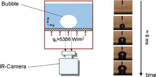
Nucleate boiling is an important type of boiling process and appears in many energy and chemical engineering applications. In order to better understand its underlying physical transport mechanisms, boiling experiments at a single artificial nucleation site have been conducted in recent years at Darmstadt University of Technology 7 (Figure 1).

Figure 1. A single-bubble nucleate boiling experiment.

In this work, we consider the estimation of the local unmeasurable boiling heat flux from high-resolution temperature measurements observed at the back of the thin heater. We use the solution approach presented in 8. A three-dimensional (3D) domain is chosen because the signal is from a thin foil of about 1 µm lateral extension with an amplitude of 10⁶ W m⁻². Thus, a vertical temperature gradient (in z-direction across the heater foil) cannot be neglected.

The estimation of the heat flux at the boiling boundary from the temperature field measured at the heated boundary belongs to the class of inverse heat conduction problems (IHCPs) 9,10, which are ill-posed in the sense of Hadamard 11. In particular, the stability condition is violated. Namely, small perturbation in the measured data leads to large deviations in the estimated quantities. In this case, a stable and hence useful solution can only be obtained using regularization strategies, such as Tikhonov regularization 12, space marching 13, function specification 9 or iterative regularization methods 14. Most of the numerical and application-oriented IHCP literature is restricted to one or two space dimensions. A selection of more recent works on 3D IHCPs 15–21 is briefly reviewed as follows. In 15, an inverse method based on the symbolic approach was proposed to determine the boundary condition in 3D IHCPs. In 16, a 3D transient IHCP was solved using the conjugate gradient method. Chantasiriwan 17 solved the inverse problem using the sequential function specification method with the assumption that future boundary heat flux varies linearly with time. A filter-based inversion method for multidimensional IHCPs was addressed in 18. Cheng et al. 19 dealt with a spherically symmetric 3D IHCP using a modified Tikhonov regularization method. Recently, the authors at RWTH Aachen University developed inversion techniques for 3D IHCPs with pointwise temperature observations 20,21. Furthermore, the numerical algorithm for solving a 3D unsteady nonlinear IHCP, the use of dynamic observers and specialized methods for the solution of anisotropic 3D IHCPs have been recently reported in literature 22–24.

Among all these methods proposed for the solution of ill-posed IHCPs, iterative regularization appears to be one of the most efficient and universal approaches 10,25. They do not require any knowledge on the character of the input data error and hence are easily applicable in practice. Here we apply one type of iterative regularization strategy based on the conjugate gradient (CG) method 8,16 to resolve the ill-posedness of the considered inverse problem. The solution method is able to systematically reconstruct the local and instantaneous heat flux distribution on the boiling surface. Its computational efficiency in 3D will become important when integrating the reconstruction of local heat fluxes from temperature measurements with the development of realistic mechanistic heat transfer models.

In the next section, we mathematically formulate the considered IHCP arising from the single-bubble nucleate boiling experiment 7. An optimization-based solution method is then presented in Section 3. A simulation case study is set up in Section 4 to validate and assess the performance of the solution method. In Section 5, we show some estimation results using real measurement data taken from the experiment sketched in Figure 1. Conclusions and an outlook are given in the final section.

2. Formulation of the inverse problem

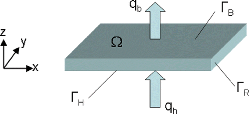
We consider the 3D domain Ω shown in Figure 2 with boundary ∂Ω = Γ_H ∪ Γ_B ∪ Γ_R, where Γ_H, Γ_B and Γ_R denote the heated, the boiling and the adiabatic boundaries of Ω, respectively.

Figure 2. Schematic representation of the 3D heating foil.

The linear heat conduction problem for the temperature T(x, t) is usually given by (1) (2) (3) (4) (5) where λ and a are the known thermal conductivity and diffusivity coefficients. T₀, q_h and q_b correspond to the initial and Neumann boundary conditions, respectively. t_f stands for the final time and the outer normal at the boundaries is denoted by n. Since the temperature variation inside the heater volume is only within a few Kelvin, it suffices to use the linear model (1–5) for the considered physical effects. Namely, instead of functions of temperature, constant values are used to model a and λ.

The IHCP corresponds to the estimation of the unknown heat flux q_b in Equations (1–5) from the measured temperature field T_m taken at the back side Γ_H of the thin heating foil. Since the heat conduction model is linear, we can reformulate the inverse problem in the following manner by dividing it into a direct problem, namely (6) (7) (8) (9) (10) which contains known initial and Neumann boundary conditions, and a reduced inverse problem with unknown q_b at Γ_B and homogenous values for the initial and other Neumann boundary conditions given by (11) (12) (13) (14) (15) The temperatures T, ū and u in the problems (1–5), (6–10) and (11–15), respectively, are related by Note that ū can be precomputed by solving (6–10) independent of the estimation process. The time used for its solution is only a negligible part of the total computational time for the whole estimation procedure. With this decomposition, the original inverse problem is reduced to the inverse problem (11–15) with unknown Neumann boundary condition at Γ_B. The corresponding temperature measurement is given by

In the following section, we discuss the chosen solution approach for the reduced inverse problem (11–15). For this purpose, we introduce the following measures for the functions f(x, t) and g(x, t) on boundary Γ, which may be either Γ_B or Γ_H depending on the context (16) (17)

3. The solution method

The motivation for the choice of this method is that it is universal and could be extended to nonlinear problems with proper modification. In contrast to standard Tikhonov regularization, which uses a regularization parameter between the residual norm and a ‘penalty term’ of the solution, here the iteration number itself is used as a regularization parameter.

Let u(x, t; q_b) be the temperature determined from the solution of Equations (11–15) with known q_b and r(x, t; q_b) being the difference between the computed and the measured temperature profiles, i.e. (18) The solution of the inverse problem (11–15) is obtained from minimizing the objective functional (19)

The CG method is used to minimize (19) by setting up an iteration sequence for the unknown heat flux function q_b(x, t) 8,16. Thus, an estimate of q_b at iteration k is computed from (20) We choose , p⁰ = ∇J⁰ as initial values for the iterative process. p^k(x, t) denotes the conjugate search direction which is updated at each iteration by (21) where the conjugate coefficient γ^k is determined from (22) Thus, at each iteration step, we need to evaluate the gradient ∇J^k and the search step length μ^k.

The gradient is obtained from (23) where the variable ψ^k satisfies the adjoint equations (24) (25) (26) (27) The function r^k(x, t) in Equation (26) denotes the computed residual (18) at the current value of q_b, i.e. . By introducing the time variable t′ = t_f − t, the final-time value problem (24–27) can be transformed to an initial value problem and hence can be solved by a standard numerical solver.

The search step length μ^k needed in (20) is computed by (28) where s^k is obtained from the following sensitivity equations: (29) (30) (31) (32)

The arising direct, adjoint and sensitivity partial differential equations (PDEs) at each iteration are solved numerically using the software package DROPS 26. Actually, due to the linearity, the temperature estimation can be updated from the identity (33) since μ^k and s^k have already been computed. Thus, Equations (11–15) with are solved only once in the first iteration. In subsequent optimization iterations, only sensitivity and adjoint problems need to be solved. This leads to a significant reduction in computational time.

In case of error-corrupted temperature measurements, the estimation quality will become worse after some iterations are applied, although the temperature residual continues to get smaller. For the choice of the best termination index, we need to apply a suitable stopping criterion such as the well-known discrepancy principle or the L-curve criterion 27,28.

The discrepancy principle suggests to stop the iterative process when the temperature residual matches the error magnitude roughly, i.e. (34) Substituting (34) into (19), we can define a threshold ε for the objective functional J in (19), i.e. (35) where A_ΓH is the surface area of Γ_H. Thus, once J < ε is satisfied at a certain iteration, the best termination index has been obtained.

An alternative method for the choice of the best termination index is the L-curve criterion, a heuristic rule, which uses a parameterized plot of the objective functional against a solution norm. Although it has been shown that the L-curve method can fail to converge, it is the preferred alternative in case the noise level of the measurement data is not known in advance.

4. A simulation case study

In this section, we set up a case study to simulate the dynamics of a ring-shaped boiling heat flux. The simulation is constructed to be similar to the settings of the real experiment 7. We consider a thin 3D domain Ω := 1 × 1 × 0.05 mm³ for computation. The known initial and Neumann boundary conditions are T₀ = 55°C and q_h = 5000 W m⁻², respectively. The same material properties are chosen as those of the heating foil used in the experiment 7, where the density ρ = 7900 kg m⁻³, specific heat c = 520 J kg⁻¹ K⁻¹ and thermal conductivity λ = 14.5 W m⁻¹K⁻¹ result in a thermal diffusivity of a = 3.53 × 10⁻⁶ m² s⁻¹. The simulation time interval is chosen as 0 ≤ t ≤ 0.05 s. The simulated heat flux (in W mm⁻²) is defined as (36) where α(t) = 0.1 sin(100π(t − 0.02)) + 0.1 for 0.015 ≤ t ≤ 0.035, zero otherwise, and for , zero otherwise. Figure 3 illustrates the temporal dynamics of the simulated boiling heat flux.

Figure 3. The exact heat flux at different time instants.

4.1. Measurement data generation

The noise-free temperature measurement is obtained by numerically solving the direct problem (1–5) with on a very fine mesh. The fine mesh is generated using piece-wise linear finite elements on a tetrahedral grid and the grid sizes in x-, y- and z-directions are all chosen as 0.005 mm. This space discretization leads to 444,411 vertices and 2,400,000 tetrahedra. The degrees of freedom are located at the vertices of the tetrahedra. The time and space discretization for the simulation case study is chosen such that the resulting discretization error is small enough. As shown by numerical experiments, the use of more unknowns in all three dimensions does only lead to negligible differences in the temperature profile inside the heater. Hence, the used grid resolution is appropriate for the prediction of the temperature dynamics. A one-step Crank–Nicolson scheme with a step size τ = 0.001 s is used for time discretization to gain a second-order accuracy. The resulting discrete systems of equations are solved with a preconditioned Krylov subspace method 29.

The perturbed version of measurements is constructed by adding an artificial measurement error to the noise-free measurement data , namely, , where σ denotes the standard deviation of the measurement error and ω is generated from a zero mean normal distribution with variance one. In this case study, different σ values, i.e. σ = 0.05, σ = 0.1 and σ = 0.2 are selected to generate noisy simulated measurement data containing different levels of noise, which correspond to measurement errors of ca. 5%, 10% and 20%, respectively. Figure 4 compares the noise-free with the noisy temperature measurements at t = 0.025 s. The simulated heat flux reaches its maximum value at this time instant.

Figure 4. The simulated temperature measurements at time instant t = 0.025 s for noise levels σ = 0, σ = 0.05, σ = 0.1 and σ = 0.2, respectively.

4.2. Estimation results with simulation data

In this subsection, we assess the performance of the solution approach presented in Section 3. To avoid inverse crimes 30, the inverse problem is solved on a coarser mesh with the grid sizes in x-, y- and z-directions chosen as 0.01 mm.

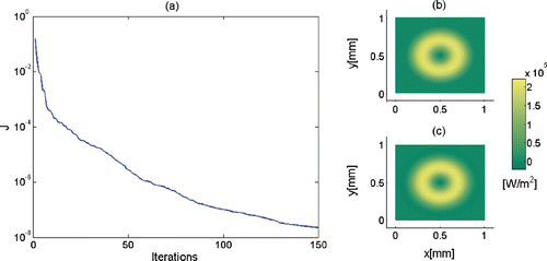
For noise-free measurement data, it is expected that the estimation quality will improve as the number of iterations increases. This is confirmed by the obtained estimation results. The convergence behaviour of the objective functional (19) is depicted in Figure 5(a). As illustrated in Figure 5(b) and (c), the difference between the exact and estimated heat flux after 150 iterations is already very small.

Figure 5. (a) Convergence behaviour for noise-free data, (b) exact surface heat flux at time instant t = 0.025 s and (c) estimated surface heat flux at time instant t = 0.025 s after 150 iterations.

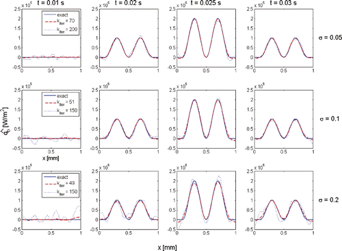
For noisy data, the application of the discrepancy principle yields the best termination indexes–iteration 70, iteration 51 and iteration 49 for measurement data with error levels σ = 0.05, σ = 0.1 and σ = 0.2, respectively. Figure 6 compares the corresponding optimal and over-estimated heat fluxes along a 2D line at Γ_B. On the one hand, for all three levels of noisy data, applying too many iterations results in worse estimation results (see the estimates obtained at iterations 200, 150 and 150 in Figure 6 for noise levels σ = 0.05, σ = 0.1 and σ = 0.2, respectively). On the other hand, the quality of the reconstructed optimal heat flux depends on the noise level of the measurement data. We observe in Figure 6 that the increase of the measurement error leads to a worse optimal reconstruction of the heat flux. Such phenomena are due to the ill-posedness of the considered IHCP.

Figure 6. Temporal evolution of optimal- and over-estimated heat fluxes along the 2D line (y = 0.5 mm) at Γ_B for measurement data with different levels of noise.

Alternatively, we also apply the L-curve criterion. In this case study, we select the solution norm defined by (16) for the estimated quantities . The resulting parameterized plots of the objective functional against the solution norms are depicted in Figure 7. The best termination indexes are found at the maximal curvatures of the three L-curves, namely at iteration 77, iteration 71 and iteration 66, respectively.

Figure 7. L-curves for estimation with perturbed measurements with error level σ = 0.05, σ = 0.1 and σ = 0.2, respectively.

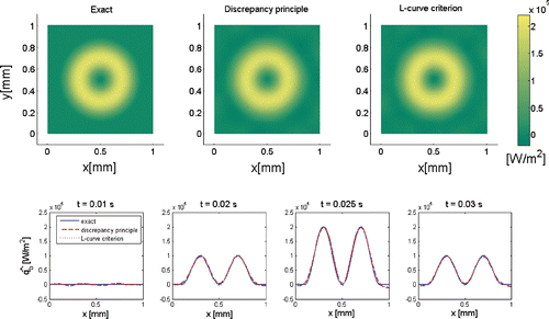
As illustrated in Figure 8, the estimated heat fluxes for data error level σ = 0.1 using the discrepancy principle and the L-curve criterion are very close. Estimation quality for other levels of measurement error are similar. The use of L-curve criterion requires to perform additional iterations after the best termination index in order to complete the curve plot. Compared to the use of the discrepancy principle, this results in more computational time. However, the L-curve criterion is superior in the case where the noise levels of the measurements are not known in advance, which is often the case in practice. In the next section, we only apply the L-curve criterion to the estimation with real experimental data whose noise level is unknown.

Figure 8. A comparison of the estimation results using discrepancy principle and L-curve criterion as stopping rules.

5. Estimation results with experimental data

In this section, we show some results obtained with real experimental data. Due to space limitations, we consider in this article only the experiments presented in 7, where the refrigerant HFC 7100 was chosen as the boiling fluid. The explicit values of the material properties have already been given in Section 4.

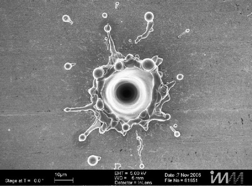
In this experiment, as shown in Figure 9, single bubbles are generated on top of a metallic foil heater (1), which is mounted onto a copper plate (3) with a circular opening (4) in the middle. The plate is fixed onto a base plate (5). Electrodes (2) are enclosed in an insolating frame (9) and pressed from both sides with grub screws (10) against the foil to guarantee good electric contact. Through the opening (4) and an IR transparent substrate (6) the bottom side of the heating foil is optically accessible. Since in this experiment nucleate boiling must be avoided at any potential sites other than the artificial one in the centre of the foil, the entire outer assembly is cooled down some degrees below saturation temperature using coolant bores (11) in the base plate (5). Ports for coolant (12) and electric current (8) are placed at the bottom side. Different types of artificial nucleation sites were examined. The experiment 7 was carried out on a 50 µm thick stainless steel foil with a bore whole of about 25 µm diameter. A scanning electron microscope (SEM) picture of the nucleation site is shown in Figure 10. The temperature field at the back side of the heater was observed with a high-speed infrared camera. The total measurement uncertainty of the IR sensor is about 0.5 K. At a resolution of 152 × 144 pixels, a frame rate of 987 Hz was applied. The resulting pixel size conforms to a square of 16 × 16 microns.

Figure 9. (a) 3D view of the foil heater. (b) Cross-sectional view of the foil heater (adapted from 7).

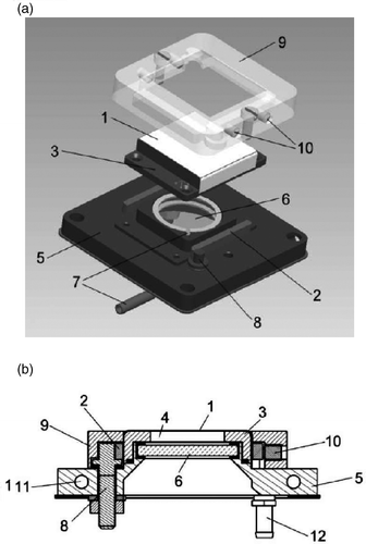
Figure 10. Nucleation site produced by laser beam at IMM (adapted from 7).

For the computation, we define a 3D domain Ω := 2.416 × 2.288 × 0.05 mm³. The space discretization follows the same resolution of the measurement data and results in 152 × 144 unknowns in the x–y-planes. The grid size in z-direction is chosen as 10 µm. It generates a total 131,328 vertices and 647,790 tetrahedra. Since 50 time frames of temperature measurements were taken with a sampling frequency of 987 Hz in the experiment, we apply a time step size of τ ≈ 1.013 ms for the time discretization.

The temperature field measured at the first time frame is used as the initial temperature distribution T₀ in Ω by assuming equal values across the foil thickness. The measured input heat flux q_h = 5356 W m⁻² is applied. The measurement was conducted with a constant heating current of 12.36 A. Since there is an unknown voltage drop at the electrodes, the heat flux was calculated using the electric resistance of the heating foil with ρ = 0.7 Ohm mm m⁻¹. The material properties for the computation have already been introduced in the simulation case study.

The measured temperature field (in K) at time frames 23, 25, 27, 29 and 31 is shown in Figure 11 (middle column). This time period corresponds to a single bubble cycle, as confirmed by simultaneous imaging with a high speed camera (Figure 11 (left column)). The noise of the scanner is 0.13 K (95% of the values are in this range). The signal has an amplitude of about 1.5 K. Thus, the signal to noise ratio is around 11.5. A cold region in the temperature distribution at frame 23 results from the activity of the previous bubble cycle.

Figure 11. Diagrams of the single bubble cycle (left), the measured temperatures (middle) and the estimated local boiling heat fluxes (right).

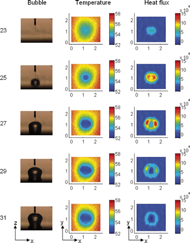
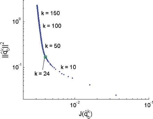
The best estimated surface boiling heat fluxes (in W m⁻²) are illustrated in Figure 11 (right column). These estimates are obtained after k_iter = 24 CG iterations with the best termination index determined from the maximum curvature point of the L-curve as illustrated in Figure 12. From the estimation results, it is apparent that the boiling heat flux undergoes a significant change during this single bubble cycle and a ring-shaped local heat flux is observed. The peak value of the estimated heat flux appears in the ring-region and is nearly 30 times higher than the average value. Since the artificial nucleate site (Figure 10) is not symmetric, the induced surface heat flux will not have the same peak magnitude in the ring-region. The peak value may be somewhat lower or higher depending on the spatial location. However, even the lower values are much higher than the macrosopic average value. These estimation results contribute towards the confirmation of the microlayer proposed by Stephan and Hammer 6. In their theory they predicted that most of the heat during boiling is transferred in the micro-region of the three-phase contact line by evaporation.

Figure 12. L-curve for the experimental data.

Near the surface boundary and in the centre of boiling surface at time frames 29 and 31, we observe small negative estimated heat fluxes. This result may be explained in different ways. The negative estimates might be an artefact of the numerical computation, in which the presented solution method intends to yield a smooth approximation for the unknown heat flux function. In case the real heat flux function is non-smooth, non-differentiable or even non-continuous at some temporal and spatial positions, small oscillating estimates around these positions will appear and this may lead to negative values. Alternatively, since the heat flux calculation is also sensitive to the electric heat input, an underestimated input heat flux q_h may also lead to negative estimated boiling heat fluxes. Thus, for more reliable interpretation, the error of the input heat flux calculation should be considered.

6. Conclusions

We have successfully applied an optimization-based identification method to estimate the local boiling heat flux in a single-bubble nucleate boiling experiment from the high-resolution measured temperature field taken on the back side of the thin heater. The presented solution approach is applicable not only for foil heaters with small thickness, but also to more thick heaters used in industrial applications. Moreover, the estimation procedure is independent of the chosen boiling fluid.

The proposed solution method is computationally efficient for 3D domains. This will be of great importance when integrating the reconstruction of local heat fluxes with model selection or parameter estimation in the entire boiling heat transfer modelling.

From the estimation results, we have observed that the boiling heat flux in a large area of the surface region undergoes little change. Although the computational cost using the considered fine mesh is acceptable, a large number of parameters show only little change in the spatial direction and are hence redundant. Future work will be devoted to reduce the number of parameters by applying a solution strategy which adaptively discretizes the computational domain during the estimation process. Reducing the number of estimation parameters is expected to not only improve the computational efficiency, but also contribute to a better regularization and consequently a better quality of the estimated quantities.

Acknowledgements

The authors gratefully acknowledge the financial support by German Science Foundation (DFG) through the research training group GRK 775 and a joint research project on fundamentals of boiling heat transfer (‘Sieden binärer Gemische’).

References

- Carey, VP, 1992. Liquid–Vapor Phase-Change Phenomena. New York: Series in Chemical and Mechanical Engineering, Hemisphere Publishing Corporation; 1992.
- Dhir, VK, and Liaw, SP, 1989. Framework for a unified model for nucleate and transition pool boiling, J. Heat Transfer 111 (3) (1989), pp. 739–746.
- Dhir, VK, 2001. Numerical simulations of pool-boiling heat transfer, AIChE J. 47 (4) (2001), pp. 813–834.
- Mei, R, Chen, W, and Klausner, JF, 1995. Vapor bubble growth in heterogenous boiling. I: Formulation, Int. J. Heat Mass Transfer 38 (5) (1995), pp. 909–919.
- Mei, R, Chen, W, and Klausner, JF, 1995. Vapor bubble growth in heterogenous boiling. II: Growth rate and thermal fields, Int. J. Heat Mass Transfer 38 (5) (1995), pp. 921–934.
- Stephan, P, and Hammer, J, 1994. A new model for nucleate boiling heat transfer, Wärme- und Stoffübertragung 30 (1994), pp. 119–125.
- Wagner, E, Sprenger, A, Stephan, P, Koeppen, O, Ziegler, F, and Auracher, H, 2007. "Nucleate boiling at single artificial cavities: Bubble dynamics and local temperature measurements". In: 6th International Conference on Multiphase Flow. Leipzig, Germany. 2007.
- Groß, S, Soemers, M, Mhamdi, A, Al-Sibai, F, Reusken, A, Marquardt, W, and Renz, U, 2005. Identification of boundary heat fluxes in a falling film experiment using high resolution temperature measurements, Int. J. Heat Mass Transfer 48 (25/26) (2005), pp. 5549–5562.
- Beck, J, Blackwell, B, and St. Clair, C, 1985. Inverse Heat Conduction. Ill-posed Problems. New York: Wiley; 1985.
- Alifanov, OM, 1994. Inverse Heat Transfer Problems. Berlin: Springer; 1994.
- Hadamard, J, 1923. Lectures on Cauchy's Problem in Linear Partial Differential Equations. New Haven: Yale University Press; 1923.
- Tikhonov, AN, and Arsenin, VY, 1977. Solutions of Ill-posed Problems. Washington: V. H. Winston and Sons; 1977.
- Raynaud, M, and Bransier, J, 1986. A new finite-difference method for the nonlinear inverse heat conduction problem, Numer. Heat Transfer 9 (1) (1986), pp. 27–42.
- Jarny, Y, Ozisik, M, and Bardon, J, 1991. A general optimization method using adjoint equation for solving multidimensional inverse heat conduction, Int. J. Heat Mass Transfer 34 (11) (1991), pp. 2911–2919.
- Yang, C, and Chen, C, 1997. Inverse estimation of the boundary condition in three- dimensional heat conduction, J. Phys. D: Appl. Phys. 30 (15) (1997), pp. 2209–2216.
- Huang, C-H, and Wang, S-P, 1999. A three-dimensional inverse heat conduction problem in estimating surface heat flux by conjugate gradient method, Int. J. Heat and Mass Transfer 42 (18) (1999), pp. 3387–3403.
- Chantasiriwan, S, 2001. An algorithm for solving multidimensional inverse heat conduction problem, Int. J. Heat Mass Transfer 44 (20) (2001), pp. 3823–3832.
- Lüttich, T, Mhamdi, A, and Marquardt, W, 2005. Design, formulation and solution of multidimensional inverse heat conduction problems, Numer. Heat Transfer Part B: Fundam. 47 (2) (2005), pp. 111–133.
- Cheng, W, Fu, C-L, and Qian, Z, 2007. A modified Tikhonov regularization method for a spherically symmetric three-dimensional inverse heat conduction problem, Math. Comput. Simul. 75 (3/4) (2007), pp. 97–112.
- Heng, Y, Mhamdi, A, Groß, S, Reusken, A, Buchholz, M, Auracher, H, and Marquardt, W, 2008. Reconstruction of local heat fluxes in pool boiling experiments along the entire boiling curve from high resolution transient temperature measurements, Int. J. Heat and Mass Transfer 51 (21/22) (2008), pp. 5072–5087.
- Egger, H, Heng, Y, Marquardt, W, and Mhamdi, A, 2009. Efficient solution of a three-dimensional inverse heat conduction problem in pool boiling, Inverse Probl. 25 (9) (2009), p. 095006.
- Loulou, T, and Artioukhine, E, 2006. Numerical solution of 3D unsteady nonlinear inverse problem of estimating surface heat flux for cylindrical geometry, Inverse Probl. Sci. Eng. 14 (1) (2006), pp. 39–52.
- Sousa, PFB, Carvalho, SR, and Guimaraes, G, 2008. Dynamic observers based on Green's functions applied to 3D inverse thermal models, Inverse Probl. Sci. Eng. 16 (6) (2008), pp. 743–761.
- Soemers, M, 2008. Numerical methods for the solution of a three-dimensional anisotropic inverse heat conduction problem. Ph.D. diss.. RWTH Aachen University; 2008.
- Kaltenbacher, B, Neubauer, A, and Scherzer, O, 2008. Iterative Regularization Methods for Nonlinear Ill-Posed Problems. Berlin: Walter de Gruyter; 2008.
- Groß, S, Peters, J, Reichelt, V, and Reusken, A, 2002. The DROPS package for numerical simulations of incompressible flows using parallel adaptive multigrid techniques. Technical Report No. 211. IGPM, RWTH Aachen University; 2002.
- Hansen, PC, 1998. Rank-Deficient and Discrete Ill-posed Problems: Numerical Aspects of Linear Inversion. Philadelphia: SIAM; 1998.
- Engl, HW, Hanke, M, and Neubauer, A, 1996. Regularization of Inverse Problems. Dordrecht: Kluwer Academic Publishers; 1996.
- Saad, Y, 2003. Iterative Methods for Sparse Linear Systems. Philadelphia, PA, USA: SIAM; 2003.
- Kaipio, JP, and Somersalo, E, 2004. Computational and Statistical Methods for Inverse Problems. New York: Springer Verlag; 2004.