Adaptive weighting input estimation of a nonlinear system

Abstract

An adaptive and robust input estimation inverse methodology for determining the time-varying unknown force, named as the input, on a nonlinear system is presented. The algorithm employs the extended Kalman filter to propose a regression model between the residual innovation and the forces. Based on this regression equation, a recursive least-squares estimator weighted by an adaptive fading factor is used to estimate the force involving measurement noise and modelling errors on-line. The capabilities of the proposed algorithm are demonstrated by numerical experiments to estimate the exciting forces acting on a nonlinear system, air-damped isolator model. Results show that the proposed method, adaptive weighting input estimation, improves the efficiency and robustness of the conventional input estimation approach.

Keywords:

• adaptive weighting input estimation
• extended Kalman filter
• recursive least-squares estimator
• conventional input estimation

1. Introduction

Nonlinear effects must be considered commonly in the design and analysis of devices and structures, to increase operating regions and improve performance. Therefore, the estimation of exciting forces in nonlinear systems is a very important task. However, the forces sometimes cannot be measured directly. The determination of the exciting forces that act on some systems from measurements of the responses of the system, through the inverse method without using intermediate force transducers, that is, the systems become their own force sensors 1, is a favourable technique. An inverse method is based on the extended Kalman filter (EKF) and a recursive least-squares estimator (RLSE) with a tuneable fading factor γ, herein, which is called the conventional input estimation (CIE) approach 2, has been successfully employed to estimate exciting forces in air-damped isolator model.

The weighting technique in RLSE is essential because the unknown force is time varying. One of the widely used weighting techniques is the fading factor γ. In the CIE approach, γ had the ability to compromise in the estimation of accuracy between the fast tracking ability and the sensitivity to noise. In the earlier studies 2, the values of γ were chosen heuristically based on an estimation of the transient status of the unknown input with a constant between 0 and 1. However, the applications were restricted to some systems that must be given a priori information about the unknown inputs. Thus, a more robust and efficient weighting input estimation algorithm is highly desirable. Some research has been done on the robust parameter estimation in which the measurements may contain outliers 3. The suitable weighting is defined based on Huber's least favourable probability density function. Huber described the measurement error in normal or long-tailed distributions, which corresponded to the noise, which was either white or outlier. When the generalized maximum likelihood estimator was linked to Huber's function, a robust weighting factor was derived that was a reciprocal function of the error 4. In this case, if we allow the weighting γ to be a function of the residual innovation at each time step, it would make a robust and adaptive estimation possible.

As generally known from earlier study of the CIE approach, the residual innovation is observable and simple and it implies the existence and quantities of unknown input. In this investigation, one proposes the correction gain analysis in RLSE to derive a quantifiable relationship between γ and innovation. The correction gain in RLSE is closely related to the bandwidth, and the bandwidth increases with a large gain 5. Thus, the RLSE transient performance is fast, but somehow at the cost of more noise in the estimation process. For small bandwidth, the disturbance was filtered, but the transient performance was slower. Now if the level of the bandwidth can be adaptively adjusted according to the residual innovation at each time step, then the aim is to find the relationship between the correction gain and residual innovation. Once the relationship is found, it is easy to construct the robust weighting algorithm by the relationship between the residual innovation and fading factor.

Herein, the efficiency of the adaptive weighting input estimation (AWIE) algorithm, developed and applied by Tuan and Hou 6 and Ma et al. 7, is illustrated by numerical simulations of the estimation of the exciting forces on air-damped isolator model 2. The estimation results of the two approaches, that is, CIE and AWIE, demonstrate that the proposed method is a highly reliable, adaptive and robust scheme.

2. Problem formulation

2.1. Discretization of a nonlinear system

In dealing with the mechanics of vibration and shock isolation, or with the design of vibration and shock isolators, the appropriate estimation of these exciting forces is a helpful task. A major cause of nonlinear behaviour in vibration problems is damping 8–10. The need for an inexpensive damper, which is operative for motion in all directions, has led to the development of the air-damped isolator 9,10. The numerical simulation example is an air-damped isolator model; (1) where m is the mass; c is the damping coefficient; k is the spring constant and F (t) is a exciting force; (t), (t) and x(t) are acceleration, velocity and displacement, respectively.

In converting to the state variable notation, according to Equation (1), the continuous-time state equations and measurement equations can be written as follows: (2) (3) where and state vector x(t) = col [x₁, x₂]; x₁ is the position; x₂ is the velocity; exciting force vector F(t) = col [0, F]; z(t) is the measurement vector; (t) is short for dx(t)/dt; the nonlinear functions f and h may depend both implicitly and explicitly on t, and herein, both f and h are assumed to be continuous and continuously differentiable with respect to all of the elements of x; w(t) is a continuous-time white noise process, and v(t_i) is a discrete-time white noise sequence.

A nonlinear dynamic system may be linearized about nominal values of its state vector. Assuming that a nominal value of x(t) and F(t) exist, x*(t) and F*(t), respectively, and its associated nominal measurement satisfy the following nominal system model: (4) (5)

Letting δx(t) = x(t) − x*(t), δF(t) = F(t) − F*(t) and δz(t) = z(t) − z*(t), when f [x(t), F(t), t] and h[x(t), t] are expanded in a Taylor series about x*(t) and F*(t), and the higher-order terms are neglected, the following perturbation state equation and perturbation measurement equation are obtained. (6) (7) where A, B and H are 2 × 2, 2 × 2 and 1 × 2 Jacobian matrices, respectively, and H[x*(t), t] =

Equations (6) and (7) constitute the linear perturbation state-variable model. Discretizing (6) and (7) yield the following discretized perturbation state-variable model, and (8) (9) where Ф is the transition matrix and Г is the input matrix. When A[x*(t), F*(t), t] is approximately constant A, during the interval t_k − t_k−1 = ΔT, (10) (11)

Furthermore, (12) where Q is the covariance of the process noise. Since the measurements are assumed to be available only at sampled values of t at t = t_i, i = 1, 2, …, Equation (7) can be expressed as Equation (9) 11,12. Also, (13) where R is the measurement noise covariance, δ_kl are the Kronecker deltas; R = σ², where σ is the standard deviation of the measurement noise, and w(k) and v(k) are mutually uncorrelated.

2.2. The CIE approach

The Kalman filter (KF) 13 was presented in 1960 and has been used extensively by engineers, scientists and managers. The filter for solving the problem of linear filtering and prediction, the dynamical system and the measurement system, are linear. However, many real-world systems are continuous in time and nonlinear. In the preceding section, a perturbation state-variable model of an air-damped isolator model was derived. Suppose x*(t) is given a prior, that is, the KF associated with using a precomputed x*(t) is known as a relinearized KF; it usually gives poor results 11. The EKF is developed in predictor–corrector format 14. The CIE algorithm has two parts – the simple EKF and the RLSE with a tunable fading factor 2. The equations for the simple EKF are (14) (15) (16) (17) (18) (19) (20) where the EKF is the prediction equation in (14), which is evaluated by means of numerical integration formulas, P(k|k − 1; *) is the state prediction error-covariance matrix, S(k) is innovation covariance, K_a(k; *) is the EKF gain matrix, P(k|k; *) is the filtering error-covariance matrix, (k) is the residual innovation and (20) is the corrector equation. Herein, because the system matrix A of the EKF is linearized about a trajectory, it is continually updated with the state estimate resulting from the measurement. The result leads to the K_a(k; *) and P(k|k; *) matrices being continually updated, as well. This is the variant for linear case 6,7.

The equations for the RLSE with a tuneable fading factor are (21) (22) (23) (24) (25) where B_s(k) and M_s(k) are the sensitivity matrices; K_b(k) is the correction gain for the updating (k); P_b(k) represents the error covariance of the estimated input vector and (k) is the estimated exciting force vector. Hence, the exciting forces can be estimated using the following three steps:

1.	Derive and identify the nonlinear state-variable model, given by Equations (1–3); the nominal system model, given by Equations (4) and (5); and discretized perturbation state-variable model, given by Equations (8) and (9), and measure the dynamic response data of the nonlinear system.
2.	Use the EKF equations, Equations (14–20), to obtain the innovation covariance S(k), innovation , and EKF gain Ka(k; *).
3.	Use the RLSE with a tuneable fading factor, Equations (21–25), to estimate the exciting forces (k).

2.3. The AWIE approach

The main aim here is to construct a robust fading factor in the algorithm, which is adaptively adjusted at each time step according to the residual innovation sequence from the simple EKF. The unknown inputs are assumed to be piecewise constant with values of F_k−1 over the interval k = 0, 1, …, m, m + 1, …, m + n, … as below: (26) where m is the on-set time of the unknown inputs. For real dynamic structural systems, the F(k − 1) might be time-invariant, or slow and rapid changes, but are usually unmeasurable. Under such situations, the proposed inverse algorithm must be able to estimate the unknown inputs robustly and efficiently. Lin 2 has already derived the recursive relation as follows: (27) where (k) = z(k) − H(k; *)(k|k − 1) is the bias-free innovations caused by measurement noise. The noises (1), …, (k) are assumed to be independent and have the same distribution, that is, white noise with zero mean values and covariances R. Also, (k) = z(k) −H(k; *)(k|k − 1) is called the bias innovation caused by measurement noise and input disturbance. (k|k − 1) and (k|k − 1) are the correspondent state estimator assuming without and with input. From Equation (27), (k) could be white or normally distributed in the absence of input. The unknown input F_k−1 can generally be arbitrary (deterministic or random). When F_k−1 starts to act on the system, the choice of the adaptive weighting γ that is related to (k) can be verified from the perspective of the frequency domain. An important result was revealed that the gain K_b(k) is the reciprocal function of γ in RLSE 15. In addition, K_b(k) increases cause the bandwidth to increase and (k) controls the level of bandwidth. It can be concluded that γ must be equal to the reciprocal function of |(k)| times a constant at each time step, described as γ_aw(k). That is, (28) where C(σ) is the tuning parameter that regulates the degree of robust of the estimator under noisy measurements. In fact, the magnitude of |(k)| is caused by measurement noise and input disturbance. According to Equation (27), (k) is normally distributed if in the absence of input. In other words, (k) behaves as the white noise when F_k−1 has not yet started. Under such a circumstance, γ_aw(k) approaches 1 and the proposed algorithm is appropriate for a time invariant input estimation 16. When F_k−1 starts to act on the system, (k) could be considered non-normally distributed owing to the coexistence of the input and noise. Now, if the quality of the sensor is not so unacceptable, the measurement noise is always smaller than the value of B_s(k)F_k−1. As generally assumed, we think σ is an acceptable threshold criterion to detect the onset of the unknown inputs efficiently. Then Equation (28) can be written as follows: (29)

The best tuning C(σ) is accomplished by the variance or sensitivity tests. The test is defined as the sensitivity of the input disturbance (k) to all the measurements equal to zero except at time t = t_p, an error with unit magnitude, that is (30)

Assume that the data errors have zero mean and constant variance σ². (k) is calculated from the exciting forces of Equation (30). If these errors were not present, all the measurements would be zero and (k) would also be zero. For the best tuning results in the least input disturbance C(σ) = σ is an efficient and acceptable choice, that is, (31)

Using Equation (31) to replace γ in Equations (23–25), we can configure an adaptive robust weighting function RLSE. Finally, the equations are (32) (33) (34)

The computational procedure to estimate the exciting forces using the proposed approach is summarized as follows:

1.	The first two steps are identical to the CIE approach.
2.	Use the RLSE with an adaptive weighting fading factor, Equations (21–22), and (32–34) to estimate the exciting forces (k).

3. Results and discussion

The numerical simulation examples are employed to evaluate the effectiveness of the proposed AWIE scheme in the preceding section. The numerically simulated examples estimate exciting forces input to Equation (1) with m = 1 kg, c = 1 N s m⁻¹ and k = 1 N m⁻¹, under a harmonic force and three types of shock – a half-sine wave shock, a rectangular shock and a triangular shock 2. The simulated parameters are follows: (1) sampling interval ΔT = 5 × 10⁻² s and final time t_f = 30 s for a harmonic force; and (2) sampling interval ΔT = 2 × 10⁻² ms and final time t_f = 20 ms for three types of shock, respectively. However, to avoid the ill-conditioned in numerical simulations of estimating shocks, the present work scaled the units, time unit is milliseconds and force is kg m ms⁻². The simulated output responses (displacements), that is, measured dynamic response data of the air-damped isolator model, using the Runge–Kutta method to estimate the corresponding the exciting forces.

The initial conditions for the both methods are generally given by (−1|−1) = col [0, 0], P(−1|−1) = diag[10¹⁰] (a 2 × 2 diagonal matrix) for the EKF, (−1) = col [0, 0] and (−1) = col [0, 0], P_b(−1) = diag[10⁸] (a 2 × 2 diagonal matrix) and M_s(−1) set to the zero matrix to which the least-squares algorithms are applied. Since P(−1|−1) and P_b(−1) are normally unknown, the estimators are initialized with P(−1|−1) and P_b(−1) as very large numbers. These selections have the effect of treating the initial errors as very large and the estimator ‘ignores’ the few initial estimates 17.

In the estimation, the AWIE and CIE approaches depend on the process noise covariance matrix Q and the measurement noise covariance matrix R. In this investigation, the CIE algorithm was first used to demonstrate the effectiveness of the fading factor γ by estimating a harmonic force and three types of shock with optimal Q and σ. The fading factor γ discards old data, which can be accomplished by weighting them according to the time they occurred. This means that the covariance of the measurement noise must somehow be increased for past measurements 18.

The error used to quantify the differences between of the exact and estimated forces, F_exact(k) and (k), is defined as follows: (35)

In this study, Equation (35) was used to evaluate the estimated results in the condition that neglected the time delay between the two time histories of the exact value and the estimated force. Here, the error is called normalized estimated error (NEE). To obtain the NEE of the optimal estimated harmonic force over time interval from 0.25 s to 30 s (deleted the initially estimated values), γ is tuned with Q = 1 × 10⁻⁴ and σ = 1 × 10⁻⁶. Figure 1 shows that the NEE of the estimated harmonic forces are 41.9–1.5%, tending to decrease as fading factor decreases from 0.9 to 0.1. That is, weighting the recent measurement most heavily and past measurements much less heavily for the estimated harmonic forces in the nonlinear system. Furthermore, to obtain the NEE of the optimal three estimated shocks over time interval from 2.5 ms to 5 ms, γ is tuned with Q = 1 × 10⁻⁶ and σ = 1 × 10⁻⁶. Figure 2 displays the NEE of the three estimated shocks are from 9.3% to 0.3%, tending to decrease as fading factor decreases from 0.9 to 0.1, similar to the results of the harmonic forces in the nonlinear system.

Figure 1. The NEE of the estimated harmonic force F(t) = sin(3t) vs fading factor for the air-damped isolator model using CIE.

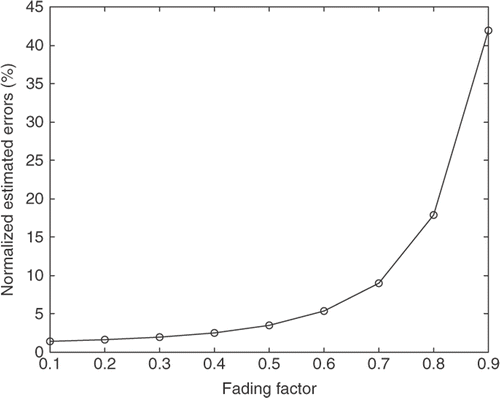
Figure 2. The normalized estimated errors of the three estimated shocks vs fading factor for the air-damped isolator model using CIE.

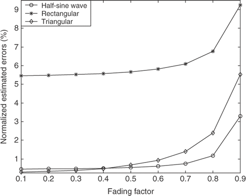
In general, it is not easy to determine the proper values Q and σ in real engineering problems. The difficulty is pronounced as one tries to give the proper choice of γ in the CIE approach to get the good estimation results. Thus, it is essential to propose a robust input estimation algorithm. In addition, as indicated in Figures 1 and 2, using γ = 0.1 in the CIE method, the estimated results of the harmonic force and three types of shock are good with Q = 1 × 10⁻⁴, σ = 1 × 10⁻⁶ and Q = 1 × 10⁻⁶, σ = 1 × 10⁻⁶, respectively. However, we could not get the good estimation results with γ = 0.9. Therefore, in numerical experiments, we have to use γ = 0.1 and γ = 0.9 to compare the efficiency and robustness of the AWIE and CIE approaches.

3.1. Simulation results

1.	For the air-damped isolator model, a harmonic force and three types of shock are estimated. Figures 3–7 show the estimated results for both AWIE and CIE approaches. Figures 3(b), 4(b), 5(b), 6(b) and 7(b) present the simulated results with γ = 0.1,Figures 3(c), 4(c), 5(c), 6(c) and 7(c) with γ = 0.9.
2.	Table 1 presents the NEE (from 0.25 s to 30 s) of the estimated harmonic force. The errors are 1.2% for the AWIE method, and 1.5% and 41.9% for the CIE method with γ = 0.1 and 0.9, respectively.
3.	Table 2 indicates the relative errors of the peak-to-peak values of the estimated harmonic force. The errors are 1.3% for the AWIE method, and 1.1% and 29.8% for the CIE method with γ = 0.1 and γ = 0.9, respectively.
4.	Table 3 reveals the NEE (from 2.5 ms to 5 ms) of the three estimated types of shock. The errors are within 5.4% for the AWIE method, and within 5.5% and 9.3% for the CIE method with γ = 0.1 and γ = 0.9, respectively.
5.	The relative errors of the estimated maximum amplitude of the three estimated types of shock are listed in Table 4. The relative errors are within 1.9% for the AWIE method, and 2.0% and 19.2% for the CIE method with γ = 0.1 and 0.9, respectively.
6.	Figure 7 presents the estimated results of the air-damped isolator model subjected to consecutive shocks over 20 ms. Note that the estimation of the consecutive shocks is effective and robust with the AWIE method.

Figure 3. The harmonic force F(t) = sin(3t) estimation of the air-damped isolator model. (a) AWIE method, (b) CIE method (γ = 0.1) and (c) CIE method (γ = 0.9).

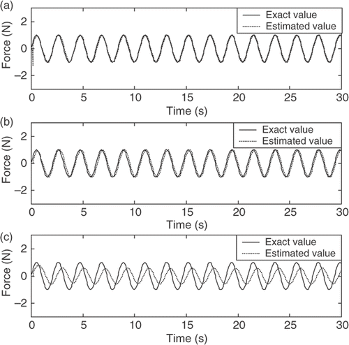
Figure 4. The half-sine wave shock estimation of the air-damped isolator model. (a) AWIE method, (b) CIE method (γ = 0.1) and (c) CIE method (γ = 0.9) (force unit, kg m ms⁻²).

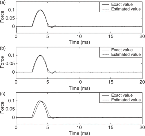
Figure 5. The rectangular shock estimation of the air-damped isolator model. (a) AWIE method, (b) CIE method (γ = 0.1) and (c) CIE method (γ = 0.9) (force unit, kg m ms⁻²).

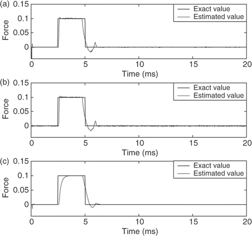
Figure 6. The triangular shock estimation of the air-damped isolator model. (a) AWIE method, (b) CIE method (γ = 0.1) and (c) CIE method (γ = 0.9) (force unit, kg m ms⁻²).

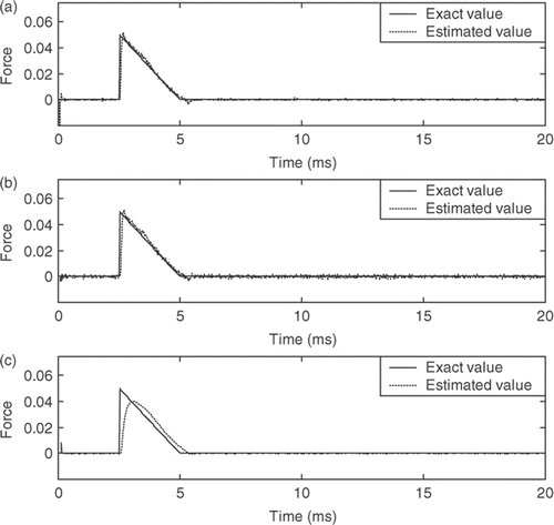
Figure 7. The consecutive loads of different magnitudes estimation of the air-damped isolator model. (a) AWIE method, (b) CIE method (γ = 0.1) and (c) CIE method (γ = 0.9) (force unit, kg m ms⁻²).

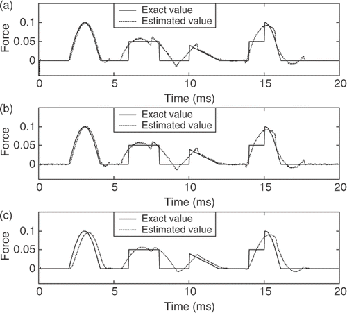
Table 1. The NEE of the estimated harmonic force F(t) = sin(3t).

NEE	CIE (%)	AWIE (%)
γ = 0.1	1.5	1.2
γ = 0.9	41.9

Table 2. The relative errors of the peak-to-peak values of the estimated harmonic force F(t) = sin(3t).

Relative errors	CIE (%)	AWIE (%)
γ = 0.1	1.1	1.3
γ = 0.9	29.8

Table 3. The NEE of the three estimated shocks.

Type of shock	NEE (%)
	CIE		AWIE
	γ = 0.1	γ = 0.9
Half-sine wave	0.5	3.3	0.4
Rectangular	5.5	9.3	5.4
Triangular	0.3	5.5	0.2

Table 4. The relative errors of the estimated maximum amplitudes of the three estimated shocks.

Type of shock	Relative errors (%)
	CIE		AWIE
	γ = 0.1	γ = 0.9
Half-sine wave	1.1	2.5	0.9
Rectangular	2.0	0.4	1.9
Triangular	2.0	19.2	1.9

3.2. Discussions of simulation

1.	As presented in Figures 3–7, the errors in the initial estimate are very large but after a few time steps the estimates rapidly converge to the exact values. These results show that the proposed scheme and the CIE method can correct the error in initial estimate using very large values of P(−1|−1) and Pb(−1).
2.	The estimated results for the AWIE and CIE methods with the proper choice γ = 0.1 show excellent agreements with the exact values of the exciting forces (Figures 3a,b, 4a,b, 5a,b and 6a,b). However, the estimated results of the CIE method with γ = 0.9 are not good (Figures 3c, 4c, 5c and 6c). Thus, we can conclude that the adaptive weighting fading factor exhibits effective and robust estimation performance.
3.	Table 2 shows the relative error of the peak-to-peak value of the estimated harmonic force for the AWIE and CIE methods. In general, the estimated results of the CIE method with γ = 0.1 are much better than those with γ = 0.9. Herein, the results indicate that the CIE method with γ = 0.9 cannot fully track the patterns of the harmonic force. On the other hand, the proposed AWIE method has good tracking capability to estimate the harmonic force, that is, the error of the peak-to-peak value is 1.3%.
4.	Table 4 shows the relative errors of the estimated maximum amplitudes for the AWIE and CIE methods. The estimated results are similar to the estimated harmonic force in the nonlinear system, that is, those in the CIE method with γ = 0.1 are much better than those with γ = 0.9. Herein, the results indicate that the CIE method with γ = 0.9 cannot fully track the patterns of the shocks. On the other hand, the proposed AWIE method has a good tracking capability to estimate the shocks, that is, the errors of the estimated maximum amplitudes are all within 1.9%. These results indicate that the estimated performance of the half-sine wave shock is more accurate than those of the rectangular and triangular shocks. The estimated error results from the rectangular and the triangular shocks change abruptly. However, the present method can still track these shocks after a few time steps, as displayed in Figures 4–6.
5.	Figure 7 reveals that the proposed method is also effective for the case when complex shock inputs are tracked.

4. Conclusions

This study presented an adaptive weighting input estimation to identify robustly time-varying exciting forces in an air-damped isolator model involving measurement and process errors. The adaptive weighting fading factor was derived as the reciprocal function of the residual innovation times a tuning constant at each time step. The examples revealed the excellent simulation results and the proposed algorithm exhibited a superior robust estimation capability over the conventional input estimation algorithm. The applications of this study are of great help in on-line condition monitoring and vibration isolation of rotating machines. Future studies will include an analysis of multi-degree-of-freedom nonlinear systems and an experimental investigation.

References

- K.K. Steven, Force identification problems-an overview. Proceedings of the 1987 SEM Spring Conference on Experimental Mechanics, Houston, Texas, USA, 14–19 June, 1987, pp. 838–844..
- D.C. Lin, Input estimation of a nonlinear system, Inverse Prob. Sci. Eng. (2010) DOI: 10.1080/17415971003698623..
- Huber, PJ, 1983. Minimum aspects of bounded influence regression (with discussion), J. Am. Stat. Assoc. 78 (1983), pp. 66–80.
- Liu, CY, Kung, MC, Chen, JC, and Chiang, SM, 1993. New robust and flexible parameter estimation method, J. Guid. Control Dyn. 16 (1993), pp. 441–413.
- Mendel, JM, 1987. Lessons in Digital Estimation Theory. Englewood Cliffs, NJ: Prentice-Hall; 1987.
- Tuan, PC, and Hou, WT, 1998. Adaptive robust weighting input estimation method for the 1-D inverse heat conduction problem, Numer. Heat Transfer, Part B 34 (1998), pp. 439–456.
- Ma, CK, Tuan, PC, Chang, JM, and Lin, DC, 2003. Adaptive weighting inverse method for the estimation of input loads, Int. J. Syst. Sci. 34 (2003), pp. 181–194.
- Inman, DJ, 1994. Engineering Vibration. Englewood Cliffs, NJ: Prentice-Hall; 1994.
- Harris, CM, 1988. Shock and Vibration Handbook. New York: McGraw-Hill Book Company, Inc.; 1988.
- Crede, EC, 1951. Vibration and Shock Isolation. New York: John Wiley & Sons, Inc.; 1951.
- Mendel, JM, 1995. Lessons in Estimation Theory for Signal Processing, Communications, and Control. Englewood Cliffs, NJ: Prentice-Hall; 1995.
- Maybeck, PS, 1979. Stochastic Models, Estimation, and Control. Vol. 2. New York: Academic Press; 1979.
- Kalman, RE, 1960. A new approach to linear filtering and predicting problem, J. Basic Eng. 82 (1960), pp. 35–45.
- Jazwinski, AH, 1979. Stochastic Models, Estimation, and Control. Vol. 2. New York: Academic press; 1979.
- Hou, M, and Xian, S, 1989. Comments on tracking a maneuvering target using input estimation, IEEE Trans. Aerosp. Electron. Syst. 25 (1989), p. 280.
- Hsia, TC, 1979. System Identification Least-Square Method. Lanham, USA: Lexington Books; 1979.
- Chan, YT, Hu, AG, and Plant, JB, 1979. A Kalman filter based tracking scheme with input estimation, IEEE Trans. Aerosp. Electron. Syst. 15 (1979), pp. 237–244.
- Gelb, AJ, Kasper, F, Nash, RA, Price, CF, and Sutherland, AA, 1978. Applied Optimal Estimation. Cambridge, MA: MIT Press; 1978.