A mollification regularization method for the Cauchy problem of an elliptic equation in a multi-dimensional case

Abstract

In this article, we consider a Cauchy problem of an elliptic equation in a multi-dimensional case. This problem is severely ill-posed: the solution (if it exists) does not depend continuously on the data. To deal with this problem, we propose a mollification method. Error estimates show that the regularized solution depends continuously on the data. Numerical examples verify that the proposed regularization strategy is effective and numerical calculation is stable in the multi-dimensional case.

Keywords:

• Cauchy problem of an elliptic equation
• ill-posed problem
• mollification method
• error estimates

AMS Subject Classifications::

• 35R25
• 35R30

1. Introduction

The Cauchy problem for the elliptic equation has been extensively investigated in many practical areas. For example, some problems relating to geophysics 1,2, plasma physics 3, cardiology 4, bioelectric field problems 5 and non-destructive testing 6 are equivalent to solving the Cauchy problem for the elliptic equation. In this article, we consider the following Cauchy problem: (1) where (2) and (3) The coefficient functions of L satisfy (4) (5) Without loss of generality, we suppose λ > 1 in this article.

Obviously, problem (1.1) is just the Cauchy problem of the Laplace equation, when a(x) = 1 and b(x) = c(x) = 0. We know that the Cauchy problem of the Laplace equation is typically ill-posed 7. Recently, there have been many numerical methods to deal with the Cauchy problem for the Laplace equation, such as the Backus–Gilbert algorithm 8, the Meyer wavelet method 9, quasi-reversibility method 10, Fourier regularization method 11 and the Tikhonov regularization method 2,12. There is no doubt that the problem (1.1) is more complex than the Cauchy problem of the Laplace equation. Here we adopt the Gauss kernel to modify the data and replace the original ill-posed problem by a new well-posed problem 13. By dint of this method, we obtain the logarithmic convergence result, and numerical results also work well as others methods.

The outline of this article is as follows. In Section 2, we analyse the ill-posedness of problem (1.1) and obtain the convergence error estimates. As we know, the ill-posedness of the solution at the end point is more serious than at the other points. Therefore, in Section 3 we give several numerical examples only at the end point x = 1, the numerical results show the effectiveness of our proposed method.

2. Regularization and error estimates

In this article, we consider the ill-posedness of problem (1.1–1.5) in the frequency space. To convert the problem in the real space into the frequency space, we need to adopt the Fourier transform for the variable y ≔ (y₁, …, y_n) ∈ ℝⁿ defined by (6) and we obtain (7) Firstly, we consider the following problem: (8) The following lemma is important.

LEMMA 2.1 14

There exists a unique solution of problem (2.3), such that

i.	υ ∈ W2,∞(0, 1), ∀ξ ∈ ℝn,
ii.	υ(1, ξ) ≠ 0, ∀ξ ∈ ℝn,
iii.	there exist positive constants ci(i = 1, 2, 3, 4) depending only on the bounds of the coefficients a(x), b(x), c(x) such that for ξ ∈ ℝn (9) (10) and if |ξ| ≥ ξ0 ≥ 0, we have where

It is easy to see that (11) is the solution of problem (2.2). We can formally write the Fourier transform of the solution ψ(y) ≔ u(1, y) of problem (1.1) at x = 1 as follows: (12) Noting (2.4b), the function υ(1, ξ) is unbounded when |ξ| → ∞. Moreover, small errors in the input data will be amplified by the factor e^|ξ|A(1), and consequently completely destroy the solution , i.e., problem (1.1) is severely ill-posed. In this article, we will apply a mollification method with the Gauss kernel to deal with problem (1.1), which we learned from Murio 13. We introduce the function (13) where α is a positive and to be determined constant. Suppose the function f ∈ L²(ℝⁿ), the convolution 13 (14) defines a C^∞ function in the entire real line. J_αf is the mollification of f. By the properties of convolution, the Fourier transform of J_αf(y) is given by (15) Moreover, there holds (16) Instead of solving the problem (1.1) with the data ϕ, we now solve the following problem with the mollified data J_αϕ^δ, where ϕ^δ is the noise data. Denoting the solution of this mollified problem by , which satisfies system (17) Similarly to solving the problem (1.1), we know that the Fourier transform of of problem (2.11) is (18) or equivalently, (19)

We considere given by (2.13) as an approximate solution of problem (1.1). We will consider the case 0 < x < 1 and x = 1, respectively. We assume that the measured data satisfies the condition: (20) and there holds the following a priori bound, (21) where E is a finite positive constant.

THEOREM 2.1

Let u(x, y) be the exact solution of problem (1.1) with the exact input data ϕ(y), and be the solution of problem (2.11). Assumptions (2.14) and (2.15) are satisfied, then we have the error estimate: (22) where c₁ and c₂ are the same as in Lemma 2.1. Furthermore, if we select (23) then for 0 < x < 1, the following error estimate holds: (24)

Proof

Using Parseval's equality, triangle inequality and Lemma 2.1, we obtain (25) Let From the above formulae, we can easily obtain (26) By elementary calculus we find that is the unique maximum point of B(ξ), so we have (27) Summarizing (2.20), (2.21), we can easily get (2.16). If we choose the parameter α by (2.17), then (2.18) holds. The proof of the theorem is completed.

To obtain the error estimate at x = 1, we introduce the following a prior assumption: (28)

THEOREM 2.2

Let u(1, y) be the solution of problem (1.1) with the exact data ϕ(y), and be the solution of problem (2.11). Assumptions (2.14) and (2.22) are satisfied, then we have the following error estimate: (29)

Proof

Using Parseval's equality and triangle inequality, we obtain the following formula: (30) where is defined (31) For the first term, by dint of (2.4a), we have (32) For the second term, on the right-hand side of (2.24) we have (33) Let We distinguish it into two cases, and take

	Case I: If |ξ| ≥ ξ0, then (34)
	Case II: If |ξ| < ξ0, then (35) Solving the equation , we have (36) So we obtain (37) Combing inequality (2.25) with formula (2.30), we complete the proof of this theorem.

LEMMA 2.3 15

Let the function g(λ) : [0, a] → ℝ be given by (38) with a constant c ∈ ℝ and positive constants a < 1, b and d, then for the inverse function g⁻¹(λ), we have (39)

Now we can choose the regularization parameter α according to i.e., (40) Denote (41) then (42) and (2.33) becomes (43) i.e., in (2.31) in Lemma 3.2. From (2.32), we obtain (44) Taking the principal part of λ by (2.37) and due to (2.34), we can easily calculate (45)

Remark 2.4

If we choose , we can obtain the following convergence estimate: (46)

3. Numerical aspect

In this section, we discuss some examples to verify the effectiveness of the proposed method. For simplicity, we consider the Cauchy problem for the Laplace equation, i.e., (47) In this case the unbounded ‘kernel’ v(1, ξ) is given by v(1, ξ) = cosh(|ξ|), ξ = (ξ₁, …, ξ_n) ∈ ℝⁿ. In all examples, we obtain the discrete noisy data ϕ^δ by adding a random noise to the input data ϕ, i.e., (48) where (49) The function “rand n(·)” generates arrays of random numbers whose elements are normally distributed with mean 0, variance σ² = 1 and SD σ = 1, ‘rand n(size(ϕ))’ returns an array of random entries that is the same size as ϕ. N is the number of the test points at x-axis. In our computations, we always take N = 101 for the one-dimension case, and N = 21 for the two-dimension case.

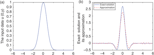
For the following examples, the noise level is ϵ = 10⁻⁴. We choose the regularization parameters α = 0.38 for the case n = 1, and we choose for the case n = 2.

Example 1

It is easy to verify that the function 11 u(x, y) = e^(x2−y2) cos(2xy) is the exact solution of Consequently, the exact solution at x = 1 is u(1, y) = e^(1−y2) cos(2y).

Usually, we cannot find an explicit analytical solution to problem (3.1), so we construct the latter examples as follows (Hào et al. adopted this kind of programme in 14): take a ψ(y) ∈ L²(ℝⁿ) and solve the well-posed problem to get an approximation to u(0, y). In detail, we use the technique of the discrete Fourier transform and inverse discrete Fourier transform combining with the formula Then we put a random noise to u(0, y) to get the noisy data ϕ^δ. Lastly, we use the proposed method to obtain the regularized solution at x = 1 and compare it with the exact solution ψ(y) to show the efficiency and stability of the proposed method.

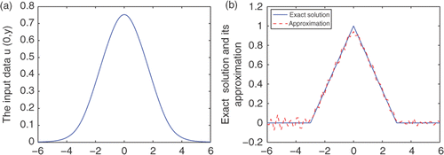
Example 2

We choose a non-smooth function

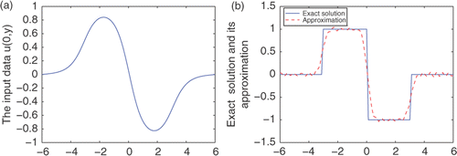
Example 3

We choose a non-continuous function

Example 4

We choose

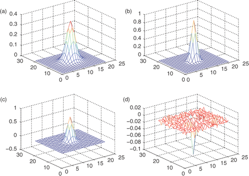
Example 5

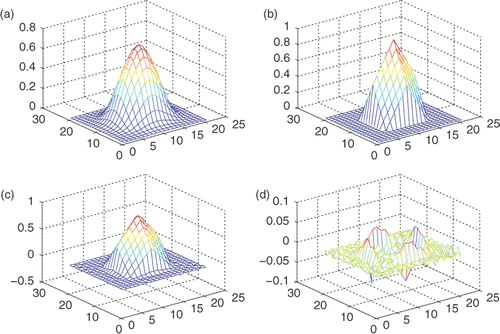
For n = 2, we choose a non-smooth function

From the Figures 1–5, we can easily see that the proposed algorithm is feasible and effective.

Figure 1. Example 1: (a) the input data ϕ, (b) exact solution and approximation.

Figure 2. Example 2: (a) the input data ϕ, (b) exact solution and approximation.

Figure 3. Example 3: (a) the input data ϕ, (b) exact solution and approximation.

Figure 4. Example 4: (a) the computed input data u(0, y₁, y₂), (b) exact solution u(1, y₁, y₂), (c) approximation, (d) absolutely error between approximation and exact solution.

Figure 5. Example 5: (a) the computed input data u(0, y₁, y₂), (b) exact solution u(1, y₁, y₂), (c) approximation, (d) absolutely error between approximation and exact solution.

4. Conclusion

In this article, we consider the Cauchy problem of an elliptic equation in a multi-dimensions case. We use the mollification method to deal with this problem, some error estimates are also given. The numerical experiments show that our proposed method works effectively.

Acknowledgements

This project is supported by the NNSF of China (Nos. 10671085, 10971089).

References

- Lavrent'ev, MM, Romanov, VG, and Shishatskii, SP, 1986. "Ill-posed Problems of Mathematical Physics and Analysis". In: Translations of Mathematical Monographs. Vol. 64. Providence, RI: American Mathematical Society; 1986.
- Tikhonov, AN, and Arsenin, VY, 1977. Solutions of Ill-posed Problems. Washington, DC: Winston; 1977.
- Gorenflo, R, 1965. Funktionentheoretische bestimmung des aussenfeldes zu einer zweidimensionalen magnetohydrostatischen konfiguration, Z. Angew. Math. Phys. 16 (1965), pp. 279–290.
- Colli-Franzone, P, and Magenes, E, 1980. On the inverse potential problem of electrocardiology, Calcolo 16 (4) (1980), pp. 459–538.
- Johnson, CR, 1997. Computational and numerical methods for bioelectric field problems, Crit. Rev. Biomed. Eng. 25 (1997), pp. 1–81.
- Alessandrini, G, 1993. Stable determination of a crack from boundary measurements, Proc. R. Soc. Edinb. A 123 (1993), pp. 497–516.
- Hadamard, J, 1953. Lectures on Cauchy's Problem in Linear Partial Differential Equations. New York: Dover; 1953.
- Hon, YC, and Wei, T, 2001. Backus-Gilbert algorithm for the Cauchy problem of the Laplace equation, Inverse Probl. 17 (2) (2001), pp. 261–271.
- Qiu, CY, and Fu, CL, 2008. Wavelets and regularization of the Cauchy problem for the Laplace equation, J. Math. Anal. Appl. 338 (2) (2008), pp. 1440–1447.
- Bourgeois, L, 2006. Convergence rates for the quasi-reversibility method to solve the Cauchy problem for Laplace's equation, Inverse Probl. 22 (2) (2006), pp. 413–430.
- Fu, CL, Li, HF, Qian, Z, and Xiong, XT, 2008. Fourier regularization method for solving a Cauchy problem for the Laplace equation, Inverse Probl. Sci. Eng. 16 (2) (2008), pp. 159–169.
- Ang, DD, Nghia, NH, and Tam, NC, 1998. Regularized solutions of a Cauchy problem for the Laplace equation in an irregular layer: A three-dimensional model, Acta Math. Vietnam. 23 (1) (1998), pp. 65–74.
- Murio, DA, 1993. The Mollification Method and the Numerical Solution of Ill-posed Problems. New York: John Wiley and Sons; 1993.
- Hào, DN, Hien, PM, and Sahli, H, 2007. Stability results for a Cauchy problem for an elliptic equation, Inverse Probl. 23 (1) (2007), pp. 421–461.
- Tautanhahn, U, 1998. Optimality for ill-posed problems under general source conditions, Numer. Funct. Anal. Optimiz. 19 (1998), pp. 377–398.