Application of a hybrid of particle swarm and genetic algorithm for structural damage detection

Abstract

This study presents a novel optimization algorithm which is a hybrid of particle swarm optimization (PSO) method and genetic algorithm (GA). Using the Ackley and Schwefel multimodal benchmark functions incorporating up to 25 variables, the performance of the hybrid is compared with pure PSO and GA and found to be far superior in convergence and accuracy. The hybrid algorithm is then used to identify multiple crack damages in a thin plate using an inverse time-domain formulation. The damage is detected using an orthotropic finite element (FE) model based on the strain energy equivalence principle. The identification is carried out using time-domain acceleration responses. The principle is to minimize the difference between the measured and theoretically predicted accelerations. Since the computational effort of identifying the use of global FE model proved prohibitive, a quarter substructure was identified which contains 72 damage variables. Using numerically simulated experiments, three cracks in a plate were reliably detected using this method in the presence of noise. While the pure particle swarm algorithm proved to be fast, the hybrid algorithm proved to be more accurate in damage prediction. GA performed worst in speed and accuracy.

Keywords:

• plates
• damage detection
• time domain
• substructure

1. Introduction

Inverse problems often occur in many branches of engineering where the values of some physical model parameters must be obtained from observed data. System identification (SI) comes under the category of inverse problem. It is the process of determining the parameters of a system based on the observed input and output (I/O) of the system. The application of SI technique presented here is the vibration signal-based damage detection of a uniform thin plate. Doebling et al. 1 presented a comprehensive survey of vibration-based damage detection methods. The development of modal analysis techniques for damage detection arose from the observation that changes in the structural properties have consequences on the natural frequencies, mode shapes and frequency response function (FRF). Many researchers have used one more of these characteristics to detect and locate damages in the structures. Lee and Chung 2 used the first lower four natural frequencies of the cantilever beam to identify a crack. Wang et al. 3 presented a damage detection scheme using static deformation and also the natural frequencies of a planar truss and beam, using an interactive optimization algorithm to locate and assess the magnitude of damages. Hwang and Kim 4 used a subset of vectors from a full set of FRFs for a few frequency measurements to detect the location and severity of the damage. Araujo et al. 5 proposed damage identification based on FRF sensitivities. The damage identification was performed on a laminated rectangular plate, discretized using finite element (FE) model. Damage in the form of a crack in an isotropic FE was expressed as an equivalent element with orthotropic properties using the strain energy equivalence principle in Ref. 6. This model was used later to predict single crack damage in a thin aluminium plate using frequency response data 7. Surface crack detection in composite laminates by the modal analysis and strain energy method was carried out in Ref. 8. Here, the FE model of composite laminate was established using ANSYS and the results are validated with experimental results. In order to deal with the computational effort in identifying systems with many unknowns, which results in large degree of freedom (DOF) models, Koh et al. 9 proposed a time-domain substructure SI scheme and presented a summary of various types of substructure approaches used for parametric SI in the time domain. The substructure approach enables us to concentrate our attention to a small zone with reduced parameters. Fewer number of sensors are required compared to full structure identification.

The original contributions of the article are summarized here. Time-domain signals have been used to identify cracks in a plate instead of frequency domain in earlier literature. Additionally, a substructure approach has been used. A hybrid of particle swarm and genetic algorithm (GA) has been used instead of pure GA or least square method in the earlier literature. This has enabled us to apply the method for problems with a larger number of damage variables.

With recent rapid advances in computer hardware and improved computational methods, applications of the inverse problem of SI and damage detection has grown rapidly. Heuristic search algorithms, such as GA and particle swarm optimization (PSO) have been applied in SI 9–12 due to their robustness in the presence of noise and ability to handle many variables. The more traditional classical methods based on calculus have been found wanting in this respect.

This article presents the application of a hybrid of GA and PSO to a time-domain damage detection scheme which detects crack damage in plates. The algorithm estimates the damage parameters through minimization of an error function defined by mean-squared error between the measured and estimated accelerations at all time steps and all locations. The measured values are obtained from an experiment; this is numerically simulated here from a known forward model where the damage location and magnitude are specified. Estimated values are obtained from the inverse model which is iteratively updated using GA or PSO or the hybrid algorithm until the model parameters match the test object.

2. GA and PSO

GAs are exploration algorithms based on the mechanism of natural selection and survival of the fittest (evolutionary principle). GA combines the explorative ability of large search spaces as well as reasonable guided search. GA creates an initial random sample within the specified domain of variables, called ‘population’. It then ranks them in the order of fitness and conducts crossover operations from among a pool of ‘parents’ through the Roulette wheel selection. Parents having higher fitness have a greater probability of being selected and their offsprings contribute to the next generation. GA can be programmed in the binary or continuous versions. Here, GA in the continuous (decimal numbers) version is used. It has been indicated in Refs 13,14 that continuous GA could outperform binary GA in computational performance.

PSO is a population-based continuous optimization technique developed by Eberhart and Kennedy 15, inspired by social behaviour of bird flocking or fish schooling (behaviourally inspired). The system is initialized with a population of random solutions and searches for optima by updating generations. However, unlike GA, PSO has no evolution operators, such as crossover and mutation. In PSO, the potential solutions, called particles, move through the problem space by following the current optimum particles. The basic PSO algorithm consists of the velocity and position equations: (1) (2) where i is the particle index, k the discrete time index, v the velocity of the ith particle, x the position of the ith particle/present solution, p_i the historically best position/solution found by the ith particle, G, the historically best position/solution found among all the particles and γ_1,2 the random number in the interval (0, 1) applied to the ith particle.

An inertia term ϕ and acceleration constants α_1,2 are also included. The inertia function is commonly taken as either a constant or as a linearly decreasing function from 0.9 to 0.4. The acceleration constants are most commonly set equal to 2. Typical values which are used in this article as PSO parameters are taken from Ref. 16.

There are some indications from previous studies of the superiority of PSO over GA. For example, the parameters of a Lorenz chaotic system were estimated using PSO 12. It was found that PSO converges to the exact value with a high population size and was more computationally efficient than GA. Likewise, a 10-DOF structural dynamic model was identified using FRFs by GA and PSO – the latter was found to be superior to the former in accuracy 17. Jiang et al. 18 divided the population into several subswarms, which are then iterated using PSO operators (position and velocity update operators), and at a periodic interval, all of those subswarms are shuffled and reassigned to subswarm. By these, the authors implemented exploration and exploitation capability to the PSO and implemented to find global optimum of benchmark functions. Ernesto and Coelho 19 presented chaotic PSO (CPSO) with chaotic sequence fuzzy model for identification of complex nonlinear system. A nonlinear thermal vacuum system of satellites was identified successfully using CPSO and the results were compared with traditional PSO.

3. The proposed hybrid method

Hybrids of various optimization algorithms have been investigated to combine the benefits of different methods. Fai et al. 20 integrated the Nelder–Mead (NM) method with GA and PSO, respectively, in an attempt to locate global optimum solution for nonlinear continuous variable function. The proposed hybrid NM–GA and NM–PSO tested on some difficult nonlinear continuous functions and NM–PSO was found to be very competitive as compared to NM–GA in finding global minimum and computational time. GA has been hybridized with various calculus-based methods to obtain a good initial guess of parameters 21,22. The Levenberg–Marquardt (LM) method is a powerful gradient-based iterative method for solving inverse problems. It tends rapidly towards the steepest descent in the neighbourhood of the initial guess. In order to obtain a good initial guess for the LM parameters, GA was hybridized with the LM algorithm 21. GA was superior in finding the global minima of the fitness function and provided the crucial initial values for the LM method. Different combinations of PSO, GA and ant colony optimization (ACO) were studied for the identification of structural parameters of beam and truss in time domain 23. The hybridization of GA and PSO was found to be far superior to all the combinations, and superior to the individual algorithms 24,25.

A chief contribution of this article is the application of a novel hybrid algorithm combining PSO and GA, for SI problems and the evaluation of its performance. GA and PSO, both start with an initial population of solutions and the hybrid combines the exploratory ability of GA (mutation, crossover) and the memory of PSO. PSO has memory as it explicitly retains the knowledge of the historically good solutions of all the particles. PSO functions by modelling the social interaction in swarms and the position of each particle (individual) is adjusted based on the knowledge of its previous best solution and globally best solution. GA simulates evolution and some individuals are selected for crossover while some others are eliminated from the generation. The PSO algorithm is conceptually simple compared GA (no selection, crossover and mutation) and can be implemented relatively easily. Taking advantage of these mutually compensating properties of PSO and GA, the above-mentioned hybrid algorithm was proposed. The proposed hybrid algorithm combines the standard velocity and position update rules of PSOs with the ideas of selection and crossover form GAs. The algorithm is designed so that the PSO performs a global search and the GA performs a local search using crossover and mutation.

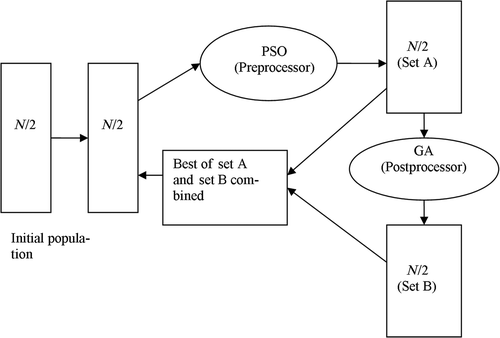
Figure 1 shows a schematic representation of the proposed hybrid PSO–GA. The hybrid algorithm operates on a net population size of N; to begin with, it uses N/2 population randomly generated as shown in Figure 1. The N/2 particles are sorted by fitness and these are fed to the PSO to create N/2 new particles (Set A). The new N/2 particles created from the PSO are used as initial population of GA and the output of GA is Set B. Now, Sets A and B are combined to get a total population of N and the N/2 best of these is passed on to PSO in the new cycle. The selection of N/2 best is explained as follows.

Figure 1. The PSO–GA hybrid algorithm.

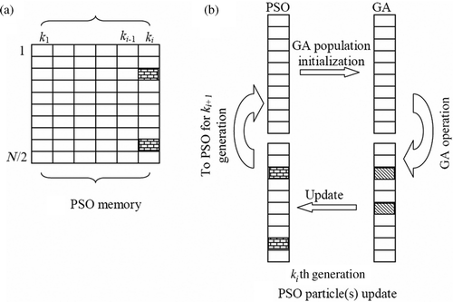
The new N individuals of the combined Sets A and B are ranked according to their fitness values. In doing so, if any particles of the PSO which have lower fitness than the new individuals created from GA, they are replaced by the new best individuals of GA. In the next PSO generation, the particle replaced by GA will be treated as gbest and the rest of the particles of PSO are scattered around it. Since PSO has memory, it stores all the particles at the end of each generation as shown in Figure 2(a). At the end of k_i generation, GA is initialized by particles created by PSO as shown in Figure 2(b). By GA operations, such as crossover and mutation new individuals are created and are compared with fitness values of PSO particles. The individuals which are found superior to the PSO (hatched cells as shown in Figure 2b) will replace the PSO particles (bricked cells) having a low fitness value. This results in incorporating expert knowledge into initialization. The updated PSO particles are stored in PSO memory after k_ith generation. These top N/2 individuals are fed to the PSO, and the process is repeated until the termination criterion is reached.

Figure 2. PSO–GA particle updating logic: (a) PSO memory and (b) PSO particle(s) update.

4. Benchmark tests

4.1. Ackley's function

The Ackley function 26 is a multimodal minimization problem. Originally, this problem was defined for two dimensions, but the problem has been generalized to n dimensions in Ref. 27. (3)

Global minimum: where a = 20, b = 0.2, e the Euler number and x_i the optimization variables.

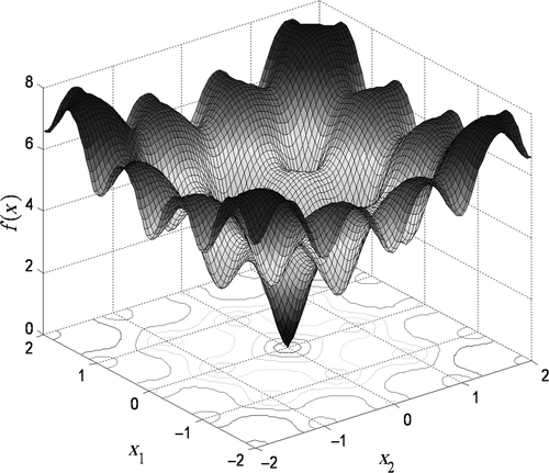
Figure 3 shows the function in a small search range of x_i from −2 to 2 for better insight into the topology of the local and global minima, whereas the full search range is from −30 to 30. As the search range increases, the function introduces many local minimums circumferentially, thereby inefficient search algorithms could converge to any one of the local minima. The global minimum of the function is zero (f(x_i) = 0) when all variables are zero (i.e. x_i = 0).

Figure 3. Ackley's function at a search range of −2 to +2.

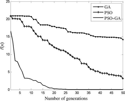
In all algorithms, termination criteria has been set to a maximum of 50 generations (iterations). PSO parameters, such as inertia function (ϕ) and acceleration constant (α) are set as a linearly decreasing inertia function from 0.9 to 0.4 and 2, respectively. The GA parameters, such as mutation rate and crossover rate are set as 1% and 40%, respectively. The combined population of the hybrid algorithm was investigated for the values of 50, 200 and 500, with the other parameters of the constituent GA and PSO parts set as mentioned earlier. Table 1 shows the summary of results of all algorithms (GA, PSO and PSO–GA hybrid) when used for optimizing Ackley's function. All the algorithms performed well when the dimension of function is small (e.g. n = 2 variables). When the dimension of function increased to 10, GA and PSO prematurely converged to suboptimal solution of f(x) = 0.0885 and 0.0062, respectively, thereby preventing the population/particles from improving. PSO–GA approached nearest the global solution of f(x)= 0.00069. When dimension n = 25, the table shows even worse performance for GA and PSO compared to PSO–GA. Figure 4(a)–(c) graphically shows the convergence for the three algorithms when n = 25 and Figure 5 shows the superior fitness function minimization property of the PSO–GA hybrid.

Figure 4. Convergence of Ackley's function variables (n = 25, search range ±30): (a)By GA, (b) by PSO and (c) by PSO–GA.

Figure 5. Ackley's function convergence by GA, PSO and PSO–GA.

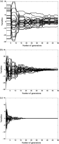
Table 1. Summary of results of Ackley's function in the final generation.

Algorithm parameters		GA	PSO	PSO–GA
Dimension, n = 2	f(x)	2.08E-06	1.21E-07	8.88E-16
Population size = 50
Dimension, n = 10	f(x)	0.0885	0.0062	0.00069
Population size = 200
Dimension, n = 25	f(x)	14.2256	3.2059	0.0041
Population size = 500

4.2. Schwefel's function

Schwefel's function is deceptive in that the global minimum is geometrically distant over the parameter space, from the next best local minima 28. Therefore, the search algorithms are potentially prone to convergence in the wrong direction and considered as difficult for most of the optimization methods. (4)

Global minimum:

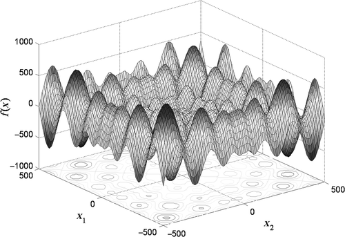
Figure 6 shows the Schwefel's function with a search range of ±500 for only two variables. It can be noticed that at the boundary there are many local minima and one global minimum of 418.9829 at x₁ = x₂ = 420.9687. When the dimension of the function increases, the density of local minima at the boundaries increase.

Figure 6. Schwefel's functions within the search range of variables x_i (±500).

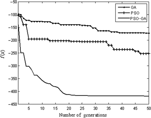
Table 2 shows the summary of results of all the algorithms (GA, PSO and PSO–GA hybrid) when used for optimizing Schwefel's function. The algorithm parameters are the same as in Ackley's function. It can be noticed that with two variables (n = 2), all the algorithms identified the global minimum (f(x) = −418.9829) correctly. With increasing dimensions (n), the GA and PSO incorrectly converge towards the local minimum of f(x) = −172.8721 and −252.836. Whereas PSO–GA converged accurately to f(x) = −418.8653 as compared to the global minimum of f(x) = −418.9829. Figure 7 shows the superior minimization of the fitness function for the hybrid algorithm compared to GA and PSO.

Figure 7. Schwefel's function convergence by GA, PSO and PSO–GA.

Table 2. Summary of results of Schwefel's function in the final generation.

Algorithm parameters		GA	PSO	PSO–GA
Dimension, n = 2		−418.9829	−418.9829	−418.9829
Population size = 50
Dimension, n = 10		−371.5510	−377.1300	−418.9829
Population size = 200
Dimensions, n = 25		−172.8721	−252.836	−418.8653
Population size = 500

4.3. Effect of population size on the convergence of objective function

The size of population has a significant effect on the convergence of the objective function. The effect of population size is studied for Ackley's and Schwefel's functions with 25 variables and are tabulated in Tables 3 and 4. If the population size is small, then the solution domain is searched less exhaustively and the algorithm gets stuck in a local minima. It can be observed from Table 3 that all the algorithms could get stuck in local minima with a population size of 50; whereas with an increase in the population size to 500, PSO–GA has converged to nearly the correct global minimum f(x) = 0. GA and PSO have fared worse. A similar trend can be observed for Schwefel's function in Table 4.

Table 3. Effect of population size on Ackley's function.

Population size	GA	PSO	PSO–GA
Ackley's (f(x))
50	20.66	10.22	2.3
100	17.86	5.74	1.82
250	14.78	4.24	0.016
500	14.22	3.205	0.0041

Table 4. Effect of population size on Schwefel's function.

Population size	GA	PSO	PSO–GA
Schwefel's (f(x))
50	−82.5142	−250.471	−413.067
100	−104.006	−294.815	−417.783
250	−215.476	−258.009	−418.25
500	−172.87	−252.836	−418.86

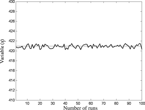
Next, the statistical analysis of the variations of one typical solution variable x_i (where i = 1 to 25, the variable number) is studied for Ackley and Schewefel's functions. Thus, Figure 8 shows the fluctuations in the solution of one variable in Schwefel's function for over 100 runs (for brevity, only Schwefel's function raw data is shown). Based on data obtained thus, the statistical results for x_i (maximum, minimum, mean and standard deviation (SD)) are tabulated in Table 5 for Ackley and Schwefel's functions. In both cases, population size of 500 and 50 generations were used. From Table 5, it is clear that hybrid PSO–GA performs better than GA or PSO with SDs of 0.003 and 0.07 for Ackley and Schwefel's functions.

Figure 8. Variation of a variable (x_i) of Schwefel's function over 100 trials.

Table 5. Statistical analysis of the benchmark function.

	GA	PSO	PSO–GA
Ackley's function
Maximum (xi)	16.154	1.003	0.011
Minimum (xi)	−19.135	−0.905	−0.008
Mean (xi)	0.045	−0.017	0.000
SD (xi)	4.859	0.316	0.003
Schwefel's function
Maximum (xi)	445.80	441.44	421.01
Minimum (xi)	196.60	398.02	420.77
Mean (xi)	380.02	420.60	420.95
SD (xi)	89.10	10.25	0.07

5. Crack damage model for damage detection in plates

After testing the algorithms using the various benchmark functions, it is proposed to apply them on a fairly complex inverse problem, i.e. the crack damage detection in a thin homogenous plate. The orthotropic damage model for thin plates presented in Ref. 6 is used here. It may be noted that this model was successfully used for crack damage detection in the frequency domain 7, i.e. using the FRFs at all the N DOFs in the global model. The method used a linear least square iterative approach which could converge to the correct value of D and θ; however, a proper initial value of D and θ has to be provided. In this article, the same crack damage model has been adapted to work with the time-domain method. Here, a substructure is modelled rather than the entire structure. Also, measurements at fewer DOFs are needed. The use of heuristic methods such as GA and PSO eliminate the need to supply the initial values of D and θ.

Based on continuum damage mechanics principle, it is shown in Ref. 6 that a small material volume (SMV) with a line crack behaves as effectively orthotropic in a small zone experiencing the same strain at the boundaries. The assumptions of this model are given below:

1.	The length of the crack is less than the length of the element.
2.	Upon the occurrence of damage, the structure continues to behave linearly.
3.	Crack is of the static type, i.e. there is no measurable growth of crack.
4.	The mass of the plate is unaffected due to crack damage.
5.	Damping is unaffected due to crack of damage.

The material behaviour of the SMV with a line crack is expressed in terms of the effectively orthotropic elastic stiffnesses, which are the functions of the isotropic elastic stiffnesses, crack orientation and the size of the line crack.

Figure 9 shows an elastic thin plate with thickness h and width L_x and L_y in the x- and y-directions, respectively. The intact plate material is isotropic and possess Young's modulus E and Poisson's ratio ν. Assume there is a line crack of length 2l at (x_D, y_D) and aligned with the crack coordinate ‘l’ which is oriented at θ with respect to the global coordinate x. The effective elastic stiffness for the SMV containing the line crack damage is shown to be: (5) where Q_ij are the reduced stiffness for the intact isotropic material in the plane stress state and e_ij the effective material directivity parameters given by (6)

Figure 9. (a) Initially isotropic plate with a line crack and (b) its equivalent continuum damage representation in terms of effective orthotropic elastic stiffness.

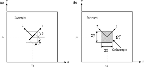
Thus, D represents the average severity of damage within an SMV, which is called herein the effective damage magnitude. The effective damage magnitude 0 < D < 1 may have two extreme values: (7) where h′ is the depth of the crack and equals h for a through crack. The effective orthotropic elastic stiffnesses given by Equation (5) are all calculated with respect to the crack coordinates 1 and 2. Thus, the effective elastic stiffness with respect to the global coordinates x and y can be obtained by using the coordinate transformation as follows: (8) where T(θ) is the coordinate transfer matrix, in which θ denotes the crack orientation (degrees) with respect to the global coordinate x. This approach has been implemented in a MATLAB-based FE model. A crack specified by the indices D and θ is assumed to be fully contained in one of the elements. The proposed damage detection scheme has to identify the location of the damaged element as well as the magnitude (i.e. D and θ values) of the crack contained by it. The range of possible values are 0 ≤ D ≤ 1 and 0 ≤ θ ≤ 90°. An undamaged element returns zero values of D and θ.

6. Inverse problem in the time domain and substructuring

In the basic time-domain damage detection approach, accelerations are experimentally measured at a few points in the structure. The accelerations are generated using a theoretical model whose damage parameters (or unknown structural parameters) are continuously updated until the difference between the theoretical and experimental models are minimized to zero at all locations and all time steps. This is a minimization problem where the optimization variables are the unknown damage variables (two damage indices per element). The hybrid algorithm is proposed to be used for this minimization. The time-domain approach can be implemented in the full structure (global model) or a reduced substructure where the damage is suspected to occur. In the latter case, all the interface accelerations need to be measured to enforce substructure compatibility. Also, a few accelerations in the interior need to be measured to compare with the experimental accelerations and formulate the minimization function. The substructure method is used here to reduce the number of unknown parameters (optimization variables) which is prohibitively large for the full model of the plate.

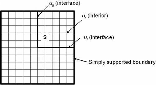
The substructure approach of Koh et al. 9,10 is used in this article and very briefly described here. Figure 10 shows the plate FE model with a quarter substructure ‘S’. The notations of the interface and interior DOF are indicated in this model. The equation of motion for the complete structural system is given by: (9) where M, C, K and P(t) are the mass, damping stiffness matrices and excitation force vector, respectively. The Rayleigh damping approach C = αM + βK, where α and β are the two coefficients decided by the user from modal information of the two global modes.

Figure 10. Global structure and substructure (S) of the plate.

Using the notations (as subscripts) ‘r’ for internal DOFs of the substructure S, ‘f ’ and ‘g’ for interface DOFs and ‘u’ and ‘d ’ for all other DOFs, the equations of motion are written in the partitioned form as follows: (10)

The above equation can be rearranged to bring the ‘interior’ partitions to the left and interface effects in the form of a force on the right as (11) with the subscript ‘j ’ denoting all interface DOFs (i.e. f and g included). This is the final form in which the substructure method is used for identification.

In the above form, it is required to measure the substructure interface displacements, velocities and accelerations (u_j terms on the right). For this, the interface accelerations have to be obtained experimentally, and thereafter integrated to obtain the displacements and velocities. Now, we can theoretically estimate any interior accelerations from the left side of Equation (11). The estimated (or predicted) accelerations at a few M interior points are thus obtained. These same interior points are required for the experimentally measured acceleration response . Using an optimization algorithm, such as the hybrid algorithm, we minimize the following fitness function, which is the sum of the square of deviations between the measured and estimated interior accelerations using the inverse method, at all locations and all time steps, (12) where subscripts ‘m’ and ‘e’ denote measured and estimated quantities, respectively, L the number of time steps and M the number of measurement sensors used. The optimization variables are the elemental properties or damage indices in the substructure. Ideally, it must be minimized to zero when the parameters of the inverse model correctly match the test object, but usually it approaches a small value close to zero.

Experiments are numerically simulated here using a known global model where the location and magnitude of crack damage are specified. The ‘experimentally measured’ accelerations at the substructure interfaces and interiors are synthetically obtained from this forward model.

7. Numerical example for damage identification

7.1. The numerical model

Figure 11(a) and (b) shows a simply supported plate with a single crack damage and three crack damages, respectively, all located in the upper right quadrant of the plate. The experimental data are synthetically generated from the forward model which incorporates these damages at the specified locations. For crack damage detection using the inverse model, the algorithm does not know the location or magnitude of the damages. The damage location is assumed to be known only at the substructure level (upper right quadrant). The damage indices (D and θ) of all the substructure elements need to be evaluated by the algorithm. The undamaged elements will give zero damage indices.

Figure 11. Aluminium plate with damage in substructure element (3,4). ⨀ Denotes acceleration measurement points at substructure interior and • acceleration measurements at substructure interface.

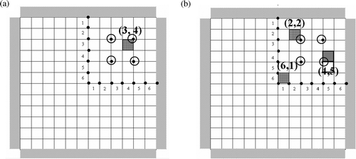
A simply supported thin aluminium plate with the following material properties is used as an example: thickness h = 0.004 m, sizes L_x = L_y = 0.5 m, Young's modulus E = 72 Gpa, Poisson's ratio ν = 0.33 and mass density 2800 kg m⁻³. This numerical example includes a forcing function from Ref. 7. A few natural frequencies of the undamaged plate are listed in Table 6. The length of the line crack and its orientation can vary from case to case. In one case, the line crack considered is 0.0332 m long and its orientation angle θ is 45°; it is located in one element at the top right quadrant of the plate (see Figure 11a). To compute the elastic stiffness for a damaged zone (SMV), the dimension of the SMV are chosen as = 0.0417 m so that the effective damage magnitude (index) for a crack length of 0.0332 becomes D = 0.5.

Table 6. Natural frequencies of simply supported plate.

Mode number	Frequency (Hz)
1	77.529
2	193.24
3	193.24
5	386.35
10	657.49
20	1163.5
30	1661.8

Table 7. Summary of DOFs of the plate structure.

	Full structure	Substructure
Total DOFs	507	147
Number of interface DOFs	−	39
Number of internal DOFs	−	108
Number of unknowns	288	72

Table 9. Summary of damage identification for three-damage case using PSO–GA and PSO (with 3% noise).

Actual		PSO–GA		PSO
D	θ°	D	θ°	D	θ°
0.3	0	0.32	0.85	0.26	1.7
0.5	30	0.47	31.5	0.55	27.3
0.7	45	0.73	46.6	0.74	44
Absolute average error (%)		5.6	4.2	9.6	5.6
Absolute maximum error (%)		6.7	5	13.3	9
Average computational time (min)		63		51

In Equation (7), D represents volume of the crack and volume of FE. The term in the denominator is area of the element (square element, ) and h′ and h (for through crack h′ = h,) are thicknesses of the crack and FE, respectively. In this study, the crack is a ‘through crack’, i.e. a crack with full depth; hence, the term πl² 7 is area of the crack, where l is half of the crack length (i.e. 2l = 0.0332 m), then the effective damage magnitude as per Equation (7) becomes 0.5.

The full plate is divided into 144 (12 × 12) FEs and the substructure (top right quarter of Figure 11a and b) consists of 36 FEs. The damage identification analysis is conducted to determine the damage magnitudes and orientations of FEs. Each element is specified by two damage indices which need to be estimated by the inverse method. Thus, the substructure has only 72 damage indices and the global structure has 288 damage indices to be estimated. Table 7 concisely shows the information mentioned above.

A point harmonic force of 10 sin(2π100t) N is applied at the centre of the plate. The excitation frequency (100 Hz) is above the first natural frequency of 77 Hz. The experiment is numerically simulated using a known forward model and the synthetic data are obtained in terms of displacement, velocity and acceleration using Newmark's method with a constant time step of 0.001 s for 2 s using the harmonic force. The simulated ‘experimental data’ was obtained numerically from the four interior points ‘r’ within the substructure (these are shown in Figure 11a and b by circles) to use in the fitness function Equation (12). Accelerations at all interface nodes are also required. The computer used was a 3-GHz Pentium 4 processor type with 1 GB RAM.

7.2. Damage identification of the single-crack model

First, the single-damage case as shown in Figure 11(a) is studied. The damaged element in the plate substructure needs to be identified for D and θ. This element is (3,4) and the exact values of D is 0.5 and θ 45°. Undamaged elements give zero values for D and θ. The performance of GA, PSO and their hybrid are compared here.

As mentioned in Table 4, the substructure consists of 36 elements and 147 DOFs. The algorithm (GA, PSO or PSO–GA hybrid) has to identify a total of 72 unknowns, namely 36 damage magnitudes (D) and 36 damage orientations (θ) for all the FEs in the substructure. The algorithm parameters and computational time taken are tabulated in Table 8. For this damage detection problem with 72 damage indices, population sizes of 500, 1000 and 1250 were tried in the same manner as for the benchmark functions whose data was shown earlier in Tables 3 and 4. It was found that a population of 1000 gave the best compromise between superior convergence and accuracy versus the limitations of the computer hardware (Pentium 4, 2.8 GHz, 1 GB RAM). Because of the significant time needed for each run, the algorithm was executed five times for each case and the average values of damage variables have been presented. All other algorithm parameters are the same as used in the benchmark functions.

Table 8. Comparison of the algorithms.

	PSO	PSO–GA	GA
Population size		1000
Number of generations		50
Computational time (min)	56.3	42.1	115.4

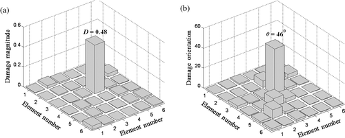
The identification results are shown in Figure 12(a) and b in three-dimensional (3-D) chart at the 30th iteration after convergence has occurred using pure PSO. The data for D is shown in Figure 12(a) and θ in Figure 12(b). PSO has identified the correct location of the damage, i.e. element (3,4) with damage magnitude, D = 0.48 and damage orientation, θ = 46°. The accuracy is good, considering the exact values of D = 0.5 and θ = 45°.

Figure 12. Damage identification – PSO 30th generation.

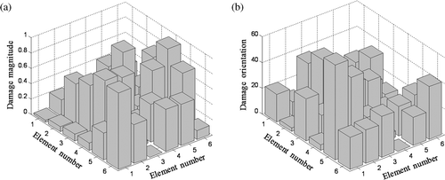
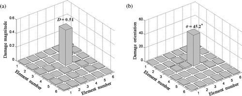
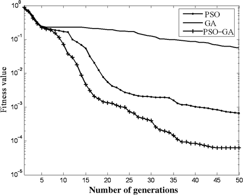
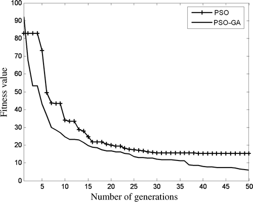
Figure 13(a) and (b) shows the identification of results by GA at the 30th iteration, which is far from converged to the final values, compared to the situation of PSO. It also incorrectly shows large non-zero damages in some undamaged elements. Next, Figure 14(a) and (b) shows the identification of D and θ using the PSO–GA hybrid in 30 generations. The results are much more accurate (D = 0.51 and θ = 45.2°) than for PSO and GA and additionally, it must be noted that the hybrid has correctly predicted nearly zero damage in all the undamaged elements. Next, we study the convergence of the fitness function of the three algorithms as shown in Figure 15. Ideally, the fitness function must be minimized to zero. It is seen that in the same number of generations, PSO–GA hybrid has minimized the fitness function to 10⁻⁴ which is better than pure PSO (10⁻³) and far better than pure GA (10⁻¹) The time taken by these algorithms for 30 generations are 56.3, 42.1 and 115.4 min (Table 8), showing that PSO–GA hybrid is rather slower than pure PSO, but much faster than pure GA. However the PSO–GA hybrid compensates the slow performance with good convergence and accuracy.

Figure 13. Damage identification – GA at 30th generation.

Figure 14. Damage identification – Hybrid PSO–GA at 30th generation.

Figure 15. Comparison of convergence of PSO, GA and PSO–GA.

7.3. Damage identification of the three-crack model

Figure 11(b) shows the three damaged elements (6,1), (2,2) and (4,5) in the plate which needs to be identified for their respective D values (0.3, 0.5 and 0.7) and θ values (0°, 30° and 45°). The excitation frequency is maintained at 100 Hz in the first case. Here, the numerically simulated acceleration ‘measurements’ are polluted with noise of zero mean and SDs of 3% to simulate experimental and modelling errors. The PSO and hybrid PSO–GA parameters are kept the same as in the previous example. The maximum number of iterations is fixed at 50.

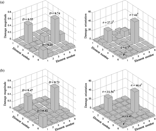
A few 3-D charts for the substructure identification are shown next. Figure 16(a) shows the damage identification using pure PSO and Figure 16(b) using PSO–GA hybrid in 50 iterations for 3% noise case. The first impression from these figures is that PSO incorrectly shows large non-zero damages in many undamaged elements, whereas this trend is much less for the hybrid algorithm. Table 9 shows the summary of damage identification results for the three-damage case using PSO–GA and PSO with 3% noise, with computational time. Now, analysing the indices of the damaged elements, referring Figure 16(a) by PSO, the identified D values 0.26, 0.55 and 0.74, which on comparing with the exact values of 0.3, 0.5 and 0.7, gives an absolute average error of 9.6% and absolute maximum error of 13.3%. The θ values identified as 1.7°, 27.3° and 44°, when compared with the exact values 0°, 30° and 45°, gives an absolute average error of 5.6% and the highest error of 9% (ignoring the zero angle). Figure 16(b) shows the results by PSO–GA with 3% noise. The D values are 0.32, 0.47 and 0.73 and θ 0.85°, 31.56° and 46.6°. They give absolute mean errors of 5.6% for D and 4.2% for θ and maximum errors are 6.7% for D and 5% for θ (much less compared to pure PSO). Pure PSO took 51 min whereas the hybrid PSO–GA took 63 min (i.e. pure PSO requires only two-third the time as the hybrid). The time requirements are more than in the previous case because of the presence of noise and requirement of more iterations.

Figure 16. Multiple damage identification with 3% noise: (a) By PSO and (b) by PSO–GA.

7.4. Statistical analysis of convergence

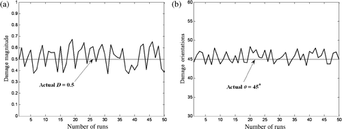
The damage detection algorithm has been executed for 50 times for the single-damage case with zero noise and multidamage cases with 3% noise using the hybrid PSO–GA. Figure 17 shows the variation of identified damage magnitude (D) and orientation (θ) for the single-damage case with noise-free measurements over 50 runs. Table 10 gives the complete statistical results obtained from this data; the mean value of D and θ are 0.52 and 46.86°, respectively. The SDs are 0.07 and 0.87. Next, the same procedure of 50 runs is repeated for the three-damage case with 3% noise. For brevity, only the statistical results of the identified damage indices of element (4, 5) are given in Table 11. The mean values of D and θ are 0.74 and 47.21°, respectively. It can be noticed that in the presence of noise, the SD of D and θ has increased to 0.11 and 2.09.

Figure 17. Variation of damage indices over 50 trials (single-damage case).

Table 10. Statistical analysis of the single-damage case of hybrid PSO–GA.

	D	θ°
Maximum	0.67	48.31
Minimum	0.37	43.38
Mean	0.52	46.86
SD	0.07	0.87

Table 11. Statistical analysis of the damage indices of element (4,5) with 3% noise.

	D	θ°
Maximum	0.89	49.45
Minimum	0.58	42.62
Mean	0.74	47.21
SD	0.11	2.09

7.5. Damage identification of a single-crack model using global approach

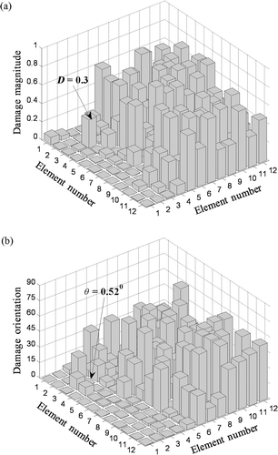
The global model contains 144 elements with 288 damage indices – a prohibitively large number of optimization variables. This difficult problem was attempted to be solved using both PSO and hybrid PSO–GA. Damage was specified at element (3,3) with D = 0.5 and θ = 0°. The population size was increased to 2000, but all other algorithm parameters were kept the same. The algorithms were allowed to continue for 50 generations; the computational time taken was 5.5 h for PSO and excess of 7 h for PSO–GA without either attaining proper convergence. Figure 18(a) and (b) shows the damage identification using PSO after 50 generations. PSO identified damage variables D = 0.26 and θ = 3.63° for the damaged element (3,3). Now Figure 19(a) and (b) shows the damage identification using PSO–GA hybrid at the 50th generation; here D = 0.3 and θ = 0.52° which is better than PSO when compared to the actual values of D = 0.5 and θ = 0°. Additionally, a quick visual comparison between Figures 18 and 19 shows that the hybrid has successfully identified some elements with non-zero damages, compared to PSO which is less successful. To gain a better insight into the behaviour of these algorithms in this difficult case, the convergence of the fitness function is plotted for both algorithms up to the 50th iteration in Figure 20. It is seen that the fitness function of PSO has a poor convergence and is almost flat after the 30th generation with no improvement. Whereas the plot for the hybrid shows a steadily decreasing trend with generations, implying a gradual improvement in results with further generations.

Figure 18. Damage identification by PSO of global structure after 50 generations: (a) Damage magnitude (D) and (b) damage orientation (θ).

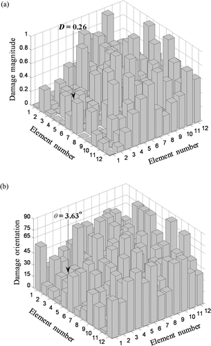
Figure 19. Damage identification by PSO–GA of global structure after 50 generations: (a) Damage magnitude (D) and (b) damage orientation (θ).

Figure 20. Convergence of fitness of global structure by PSO and hybrid PSO–GA.

However, 288 optimization variables cannot be accurately solved using the available methods (including increasing the generations beyond the hardware capability of the computer). This example is only shown to illustrate the advantage of substructure method. In case full structure is to be identified, then one has to use the ‘divide and conquer’ approach, i.e. divide the structure into small substructures and identify them separately.

8. Conclusions

In this article, a novel hybrid optimization algorithm combining GA and PSO is successfully applied to time-domain damage identification. Using the Ackley and Schwefel multimodal benchmark functions, the superiority of the hybrid over conventional GA and PSO was established for up to 25 variables. The algorithm was then applied to a more challenging problem of identifying crack damages in elements of a plate. A substructure approach is used to save computational effort, and the crack damage mechanics was simulated using the strain energy equivalence principle, whereby a damaged element was represented as an effectively orthotropic element, which is the function of crack damage magnitude and orientation. There are 72 damage variables to identify which is quite large for an optimization problem. The hybrid algorithm was able to correctly predict the location and damage magnitude and angle at simultaneously three different locations in the plate, with noise in the measurements. In the more challenging problem of identifying 288 damage variables in the global model, the hybrid algorithm showed a significant promise of solution with future generations, whereas the PSO was completely stuck in some local optima.

References

- Doebling, SW, Farrar, CR, Prime, MB, and Shevitz, DW, , Damage identification and health monitoring of structural and mechanical systems from changes in their vibration characteristics: A Literature review, LA 13070 MS, Los Alamos National Laboratory 1996.
- Lee, Y-S, and Chung, M-J, 2000. A study on crack detection using eigenfrequency test data, Comput. Struct. 77 (2000), pp. 327–342.
- Wang, X, Hu, N, Fukunaga, H, and Yao, ZH, 2001. Structural damage identification using static test data and changes in frequencies, Eng. Struct. 23 (2001), pp. 610–621.
- Hwang, HY, and Kim, C, 2004. Damage detection in structures using few frequency response measurements, J. Sound Vib. 270 (2004), pp. 1–14.
- Araujo dos Santos, JV, Mota Soares, CM, Soares, CA, and Maia, NMM, 2005. Structural damage identification in laminated structures using FRF data, Compos. Struct. 67 (2005), pp. 239–249.
- Lee, U, Lesieutre, GA, and Fang, L, 1997. Anisotropic damage mechanics based on strain energy equivalence and equivalent elliptical microcracks, Int. J. Solid Struct. 34 (1997), pp. 4377–4397.
- Lee, U, Cho, K, and Shin, J, 2002. Identification of orthotropic damages within a thin uniform plate, Int. J. Solids Struct. 40 (2002), pp. 2193–2213.
- Hu, H, Wang, B-T, Lee, C-H, and Su, J-S, 2006. Damage detection of surface cracks in composite laminates using modal analysis and strain energy method, Compos. Struct. 74 (2006), pp. 399–405.
- Koh, CG, Hong, B, and Liaw, CY, 2003. Substructural and progressive structural identification methods, Eng. Struct. 25 (2003), pp. 1551–1563.
- Koh, CG, See, LM, and Balendra, T, 1991. Estimation of structural parameters in the time domain: A substructure approach, Earthquake Eng. Struct. Dyn. 20 (8) (1991), pp. 787–801.
- Hao, H, and Xia, Y, 2002. Vibration based damage detection of structures by genetic algorithm, J. Comput. Civil Eng. 16 (3) (2002), pp. 22–229.
- He, Q, Wang, L, and Liu, B, 2007. Parameter estimation for chaotic systems by particle swarm optimization, Chaos, Solitons Fractals 34 (2007), pp. 654–661.
- Michalwicz, Z, 1994. Genetic Algorithms + Data Structures = Evolutionary Programs. New York: AI Series, Springer-Verlag; 1994.
- Haupt, RL, and Haupt, SE, 1999. Practical Genetic Algorithms. New York: John Wiley and Sons; 1999.
- Eberhart., RC, and Kennedy, J, , A New Optimizer using Particle Swarm Theory, Proceedings of the 6th International Symposium on Micro Machine and Human Science, Nagaya, Japan, 1995.
- Shi, Y, and Eberhart, R, , Parameter Selection in Particle Swarm Optimization, Proceeding of the 7th Annual Conference on Evolutionary Programming, EP98. San Diego, USA, 1998.
- Mouser, CR, and Dunn, SA, 2005. Comparing genetic algorithm and particle swarm optimization for inverse problem, ANZIAM J. 46 (E) (2005), pp. 89–101.
- Jiang, Y, Hu, T, Huang, CC, and Wu, X, 2007. An improved particle swarm optimization algorithm, Appl. Math. Comput. 193 (1) (2007), pp. 231–239.
- Araujo, E, and Coelho, LDS, 2008. Particle swarm approaches using Lozi map chaotic sequences to fuzzy modelling of an experimental thermal-vacuum system, Appl. Soft Comput. 8 (4) (2008), pp. 1354–1364.
- Fai, SKS, Liang, YC, and Zahara, E, 2006. A genetic algorithm and a particle swarm optimizer hybridized with Nelder-Mead simplex search, Comput. Ind. Eng. 50 (2006), pp. 401–425.
- Friswell, M, Penny, I, and Garvey, SD, 1995. A combined genetic and eigen sensitivity algorithm for the location of damage in structures, J. Sound Vib. 186 (1995), pp. 311–323.
- Kishore, R, Sandesh, S, and Shankar, K, 2007. Parametric identification of nonlinear dynamic systems using combined Levenberg-Marquardt and genetic algorithm, Int. J. Struct. Stab. Dyn. 7 (4) (2007), pp. 715–725.
- Sandesh, S, Sahu, AK, and Shankar, K, 2009. Structural system identification in the time domain using behaviorally inspired algorithms and their hybrids, Int. J. Eng. Res. 6 (2) (2009), pp. 64–67.
- Gaafar, LK, Masoud, SA, and Nassef, AO, 2008. A particle swarm-based genetic algorithm for scheduling in an agile environment, Comput Ind. Eng. 55 (3) (2008), pp. 707–720.
- Marinakis, Y, and Marinaki, M, 2010. A hybrid genetic – Particle swarm optimization algorithm for the vehicle routing problem, Expert Syst. Appl. 37 (2) (2010), pp. 1446–1455.
- Ackley, DH, 1987. A Connectionist Machine for Genetic Hill Climbing. Boston: Kluwer Academic Publishers; 1987.
- Bäack, T, 1996. Evolutionary Algorithms in Theory and Practice. UK: Oxford University Press; 1996.
- Schwefel, HP, 1981. Numerical Optimization of Computer Models. New York: John Wiley and Sons; 1981.