Inverse computation of cohesive fracture properties from displacement fields

Abstract

The cohesive zone model (CZM) is a key technique for finite element (FE) simulation of fracture of quasi-brittle materials; yet its constitutive relationship is usually determined empirically from global measurements. A more convincing way to obtain the cohesive relation is to experimentally determine the relation between crack separation and crack surface traction. Recent developments in experimental mechanics such as photoelasticity and digital image correlation (DIC) enable accurate measurement of whole-field surface displacement. The cohesive stress at the crack surface cannot be measured directly, but may be determined indirectly through the displacement field near the crack surface. An inverse problem thereby is formulated in order to extract the cohesive relation by fully utilizing the measured displacement field. As the focus in this article is to develop a framework to solve the inverse problem effectively, synthetic displacement field data obtained from finite element analysis (FEA) are used. First, by assuming the cohesive relation with a few governing parameters, a direct problem is solved to obtain the complete synthetic displacement field at certain loading levels. The computed displacement field is then assumed known, while the cohesive relation is solved in the inverse problem through the unconstrained, derivative-free Nelder–Mead (N–M) optimization method. Linear and cubic splines with an arbitrary number of control points are used to represent the shape of the CZM. The unconstrained nature of N–M method and the physical validity of the CZM shape are guaranteed by introducing barrier terms. Comprehensive numerical tests are carried out to investigate the sensitivity of the inverse procedure to experimental errors. The results show that even at a high level of experimental error, the computed CZM is still well estimated, which demonstrates the practical usefulness of the proposed method. The technique introduced in this work can be generalized to compute other internal or boundary stresses from the whole displacement field using the FE method.

Keywords:

• cohesive zone model
• inverse problem
• optimization
• Nelder–Mead method
• digital image correlation

1. Introduction

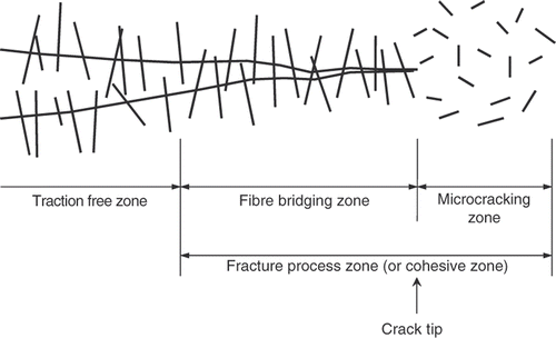
Quasi-brittle materials, such as plastics, concrete, asphalt or adhesives, usually show non-linear load-deformation behaviour and a gradual decrease of load capacity (softening behaviour) after peak load. The relatively ductile behaviour of quasi-brittle materials is due to the development of a fracture process zone (size of which may be comparable to the size of the specimen) in front of the macroscopic cracks. For example, Figure 1 illustrates a fracture process zone formed due to fibre bridging and micro-cracking. Linear elastic fracture mechanics (LEFM) is inadequate when taking account of the non-linear characteristic of such a fracture process zone.

Figure 1. Illustration of the fracture process zone in a typical fibre-reinforced composite.

A popular fracture mechanics model that accounts for the process zone behaviour is the cohesive zone model (CZM) 1,2, which has also been referred to as the fictitious crack model 3. In the finite element (FE) context, the elastic deformation is represented by the bulk elements, while the cohesive fracture behaviour is described by cohesive surface elements. Both ‘intrinsic’ models 4,5 and ‘extrinsic’ models 6–8 have been developed. Moreover, the CZM concept has also been implemented in conjunction with extended and generalized FE methods (X-FEM and GFEM) 9,10. The method has been successfully applied to various types of materials including polymers 11,12, concrete 13, functionally graded materials 14 and asphalt 15,16. Here, the CZM concept is explored with emphasis on quasi-brittle material systems.

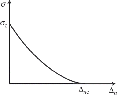
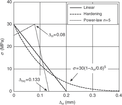
Commonly used in the simulation of mode I and/or combined fracture modes, the CZM describes a material level constitutive relation for the idealized damage process zone which applies only to the fracture surface, while the undamaged bulk material remains elastic. For mode I fracture, the CZM assumes a relation between normal traction and crack opening displacement (COD; Figure 2), while for pure mode II, the relation is between shear traction and sliding displacement. In Figure 2, Δ_n denotes COD, σ denotes the cohesive traction/stress, Δ_nc and σ_c are the critical values of Δ_n and σ, respectively, and σ(Δ_n) describes the traction–separation relation. The CZM may be obtained through experiments, either directly or indirectly.

Figure 2. Crack surface tractions (mode I).

Many approaches have been proposed to obtain the curve σ(Δ_n). Experimentally, the direct tension test may be considered the most fundamental method to determine σ(Δ_n) 17,18. However, this approach is extremely difficult 17,19, which led researchers to seek indirect methods. Another direct method involves relating crack tip opening displacement to energy release rate and then differentiating such relationship to obtain σ(Δ_n). Other methods employ inverse analysis and one common procedure relies on assuming a simple shape of σ(Δ_n) with a few model parameters. Independent investigations by Song et al. 16 and Volokh 20 demonstrate that the assumed CZM shape can significantly affect the results of fracture analysis. Moreover, Shah et al. 19 reviewed various shapes of σ(Δ_n) that have been proposed, which include linear, bilinear, trilinear, exponential and power functions, and concluded that the local fracture behaviour is sensitive to the selection of the shape σ(Δ_n). These models include a few parameters that are either computed directly from experimental measurements or indirectly by inverse analysis.

Some earlier efforts in inverse computing the CZM have been focused on the well-defined two- or three-branch piecewise linear softening models for mode-I fracture 21–25. The two-branch model has actually been recommended by RILEM and it involves four unknown parameters to be identified (the three-branch model involves six unknown parameters). Three-point bending and wedge splitting tests are usually used for the inverse analysis, either numerically or experimentally. Sophisticated algorithms are used to solve the inverse problems, e.g. Kalman filter 21 and non-linear programming approaches 24,25.

van Mier 26 summarized the common procedure of inverse analysis: model parameters are adjusted at each iteration by comparing the difference between the computational and experimental outcomes of global response. This method is not computationally efficient since a complete simulation must be carried out at each iteration. Recently, Elices et al. 27 summarized the main streams of the indirect methods used to determine σ(Δ_n). These indirect methods have common characteristics: they all use the global response of the experimental results, load (P) and displacement (δ) or crack mouth opening displacement (CMOD), from popular notched beams or compact specimens, as the basis of the inverse parametric fitting analysis. This is simply because the global responses are usually the only obtainable outcomes of experiments. Therefore, the limitations are manifested: these methods are semi-empirical in that the CZMs are assumed, a priori, and they cannot be validated confidently at the local level. This also implies less confidence on the uniqueness of the obtained CZM. However, the obtained CZM from these methods still yields satisfactory predictive capability in FE simulation of fracture 13,28,29.

1.1. Motivation: digital image correlation

Fundamentally, stress can only be measured indirectly, while displacement or strain is traditionally measured at limited number of discrete points. Recent developments in experimental stress analysis techniques, such as photoelasticity, laser interferometry and digital image correlation (DIC), enable measurements of whole deformation field 30. The rich experimental data have attracted the attention of researchers who work on inverse identification problems 31,32. Among these techniques, DIC shows great potential in experimental fracture analysis 33–35.

Recent hardware and software developments of DIC techniques enable researchers to obtain submicron measurement of two-dimensional (2-D) whole displacement field on a flat specimen surface. Such accurate measurement of displacement field allows one to take numerical derivatives to obtain strain field, though it may introduce errors in the process of differentiating experimental data. The stress is then obtained using the known elastic properties. In such a way, stress near the crack surface can be obtained to approximate the cohesive stress. By statistically correlating the COD with the cohesive stress, one can obtain the CZM from the local level 35. This scheme correlates cohesive stress with COD in a discrete fashion without considering the possible influence from adjacent materials, which may degrade the accuracy. Also, for stiff, brittle materials, the failure stress of the material is normally very low and the associated strain level in the bulk material is therefore always low. This can lead to extreme difficulty in obtaining derived strain accurately.

More sophisticated methods for the inverse parameter identification problems involve combining FE method and continuous deformation field. Some well-developed methods are: constitutive equation gap method 36, equilibrium gap method 37, finite element model updating (FEMU) method 38,39 and virtual fields method (VFM) 40. These methods have been reviewed and compared recently 32,41. The comparative study between these methods shows that the FEMU and VFM yields consistently the accurate estimation of the target constitutive parameters. The VFM is a non-updating method, which is computationally efficient; however, it requires relatively accurate whole-field displacement measurement. The FEMU method is an updating approach, which begins with an initial guess and iteratively updates the constitutive parameters by minimizing a prescribed cost function. Usually, the cost function for the FEMU is a least-square difference between the measured displacement field and the computed counterparts. A whole-field displacement is not necessarily required for the FEMU approach, but the availability may improve the accuracy of the identification. These methods have been primarily applied to the identification of distribution of elastic moduli, model parameters and imbeded objects, and have not been applied to identify the CZM.

Motivated by the access to the full displacement field obtainable from DIC and by the power of FE simulations of fracture phenomena, the idea of combining DIC with the FEM adopting the robust FEMU method is explained in this investigation. The key idea is to utilize the full displacement field in an FEM frame. Avoiding the computation of the stress from the derived strain field (a potentially significant source of errors) is the major advantage of using FEM. The proposed scheme is described in the next section.

1.2. Proposed procedure

The investigation of the proposed scheme to compute CZM is carried on a 2-D FEM of four-point single edge-notched beam (SENB) specimen for convenience. We assume that there is only mode I fracture with one crack along the symmetry line of the specimen, where the CZM is implemented. As an additional note, the proposed method also applies to other geometries where only mode I fracture is present and the crack path/paths are known a priori, such as the popular three-point bending and the wedge splitting tests.

In the direct problem, we assume a known CZM. An intrinsic CZM implementation is then used to solve the non-linear fracture process, results of which include global load (P) versus CMOD and the displacement field at each loading step. The inverse problem uses the displacement data at the nodal points of the FEM of the SENB specimen (which is a large number of data with refined FE meshes) corresponding to certain post-peak points in the P versus CMOD curve, where the full cohesive zone is formed. The global response curves, either P versus CMOD, or P versus load–line displacement, are not used in the inverse identification.

In the inverse problem, the CZM is the unknown while the displacement data, recorded at every node, from the direct problem is treated as synthetic experimental data. Synthetic errors are added to the displacement data before it is used in the inverse analysis. The inverse problem is formulated as an unconstrained optimization problem in which a flexible CZM shape representation defined by a set of unconstrained parameters is to be optimized.

The remainder of this article is organized as follows. In Section 2, first, the direct problem is briefly presented. Subsequently, we focus on the presentation of the inverse problem: parameterization of the CZM using splines is first presented; the formulation of inverse problem is elaborated; the Nelder–Mead (N–M) solver and the augmented objective functions are then explained; finally, the assistance to optimization is briefly presented. In Section 3, the results of the direct problem are first presented and briefly discussed. The rationale of adding errors is then described in detail. For the results, the focus is on the effect of different levels of errors and the practical way of using experimental data. Then some numerical aspects of the inverse procedure are briefly discussed. Finally, conclusions are made summarizing the contribution of this study.

2. Problem description

2.1. Direct problem: ‘synthetic’ problem

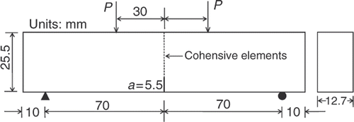
Figure 3 shows the geometry of the SENB specimen. The problem considered currently is in a 2-D plane-stress condition. The bulk material is presumed isotropic and linear elastic. Since the relative accuracy of the DIC measurement also depends on the stiffness of the bulk material, three moduli of elasticity are considered: E = 10, 30 and 100 GPa. The Poisson's ratio is fixed as 0.2.

Figure 3. Geometry of the SENB and the test set-up.

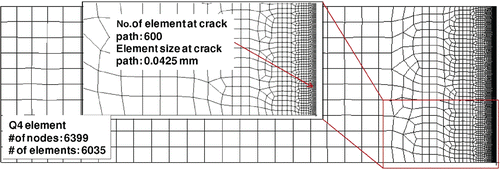
The subsequent analysis uses a 2-D FEM. Fine meshes are used to simulate the level of detail for the displacement field that could be obtained by the DIC technique. Figure 4 shows the mesh used for both the direct and inverse problems, where Q4 elements are utilized for the bulk material and the CZM is implemented for mode I fracture only. The size of the element (bulk material) along the crack surface is 0.0425 mm, which is fine enough to yield accurate crack propagation simulation.

Figure 4. FEM mesh for the half of the geometry (due to symmetry).

2.1.1. Idealized CZMs

Idealized CZMs describing three representative behaviours are used (Figure 5): one with a linear softening behaviour, one with a hardening (HD) then followed by a linear softening behaviour and one with a power-law (PL) softening behaviour. The linear CZM is appropriate for the high explosives 35, the PL CZM is effective to simulate the fracture process of quasi-brittle concrete 42, while the HD CZM may be used for some strong fibre-reinforced composites 18,43.

Figure 5. The mode I CZMs used in this study.

2.1.2. Basic formulation

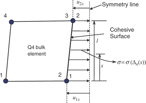
Figure 6 shows one bulk Q4 element aligned to the cohesive surface, where σ denotes the mode I cohesive stress. For this Q4 element (1) where is the bulk element stiffness matrix, u^e is the element nodal displacement and r is the element nodal force. When the cohesive stress is the only stress contributing to r, we have (2) where s is the local natural coordinate shown in Figure 6, l is the size of the Q4 element, t is the beam thickness, k_c = σ/Δ_n, is the shape function in natural coordinate system, and . The vector denotes the nodal displacement in the x direction, and denotes the cohesive element stiffness matrix.

Figure 6. A bulk Q4 element along the cohesive surface interface.

As , , can be simplified: (3) where is the shape function in the isoparametric coordinate system.

Equations (1) and (2) give the contributions of each element to the cohesive and bulk stiffness, and the global system of equations becomes (4) where K_b is the global stiffness matrix of the bulk material, K_c is the global cohesive stiffness matrix, u is the global displacement vector and F^ext is the global external force vector.

The sequence of iterations for the displacement field u at a specified load can be obtained through (5) where n is the nth loading step and m is the mth iteration for the current loading step.

2.2. Inverse problem

2.2.1. Shape representation of CZMs

We aim to extract CZM without making any assumption about its shape. This approach is desirable since we usually have limited knowledge of the cohesive property of new materials or material systems.

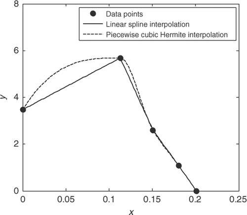
We propose the use of splines to describe the CZM, i.e. the relation of traction–separation. Two common spline interpolations are used (Figure 7): linear spline (LS) interpolation, which is equivalent to linear interpolation, and piecewise cubic Hermite (PCH) interpolation to offer choices on the type of description, e.g. polylinear or smooth. Detailed information of PCH interpolation can be found in 44,45.

Figure 7. Illustration of various interpolation schemes.

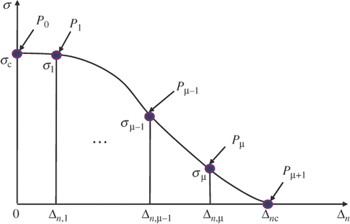
The use of splines allows for a shape representation based on an arbitrary number of control points. Let us define the coordinates of the μ + 2 control points according to Figure 8, i.e. which leads to the unknown physical CZM parameters as (6)

Figure 8. Parameterization for splines.

2.2.2. Optimization approach

Irrespective of the knowledge of the CZM shape, both the direct and the inverse problem can be expressed in the form (7)

In the inverse problem, the unknown to solve for is the set of parameters λ that describes the CZM. Denoting by the displacement vector representing the whole displacement field already available, either from the direct problem, or from experimental measurement, e.g. from DIC, Equation (7) can be rearranged as (8) where the following notation is introduced: (9) Now the cohesive stress is considered as boundary stress and is accounted for in the new global external force vector, . One intuitive way to solve this problem is through minimizing the norm of the residual defined as (10) However, K_b as an operator being applied to discards the rigid-body-motion part of , and K_b also significantly magnifies the errors exiting in . To circumvent such pitfalls, we propose to search for λ as follows: (11) where M is the number of input parameters and Φ(λ) is the objective function, is the Euclidean norm of a vector, c_i(λ) are the constraint functions, L is the number of constraint functions and w_u is the vector of weighting factors and u*(λ) is computed by (12) The external force vector can be computed in the following manner. First, from , the COD vector Δ_n for all nodes at crack surface can be extracted directly. With a known λ, the CZM function is defined. Then the first part of Equation (2) is used to compute the equivalent element nodal force vector of the cohesive stress. By assembling all the element nodal force vectors, can be obtained. Equation (12) can be evaluated efficiently by first factorizing the constant matrix K_b.

The weighting vector shall reflect the physical significance of every single parameter. Displacement field near the crack is more directly influenced by the cohesive properties. Therefore, the corresponding displacement sample points shall be given higher weights. However, it is not easy to determine a threshold boundary for significant cohesive influence region. As a simple start, a vector of uniform weighting factors is used. The numerical results presented in this article have shown the applicability of the uniform weighting factors.

2.2.3. The N–M solver

The N–M optimization method 46–48, an unconstrained and derivative-free optimization method, is utilized to solve Equation (11). An initial guess of the CZM parameters λ is provided to the N–M solver, which carries out the procedure described below. The stop criterion of the N–M algorithm can be set by comparing the best simplex vertex (explained in the next paragraph) or the value of Φ(λ) between adjacent iterations, or be set by when value of Φ(λ) is sufficiently small.

For an objective function to be minimized, a simplex of M + 1 vertices is first formed. A simplex in is a line segment, in is a triangle, in is a tetrahedron, and so on. Let be the initial guess/point, which is also a vertex of the simplex to be formed. The other vertices can be selected by making parallel to the ith M-dimensional unit vector , in which ‘1’ appears as the value of the ith component. The length of the vector can be a typical length scale in ith dimension. This way, , , … ,  are mutually normal to each other, i.e. points λ₀, λ₁, … , λ_M are not coplanar in the Euclidian space.

At any stage, the N–M method aims to remove the vertex with the largest function value and to replace it with a new vertex with a smaller function value. This procedure guarantees that the average objective function value at each step is non-increasing.

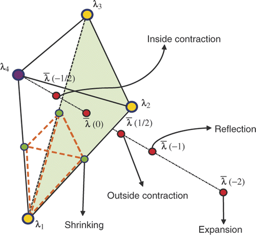
Figure 9 demonstrates the algorithm of N–M method for one step. Vertices λ₁, … , λ₄ are ordered such that . We say point λ_i is better than point λ_j if . The centroid of the best three points is . Any point along the line joining points λ₄ and can be defined by . One commonly used scheme is to replace λ₄ with one of the four points along the line: expansion point , reflection point , outside contraction point or inside contraction point . The details of which point to replace could be found in reference 48. If all those four points are still worse than λ₄, shrinking of points λ₂ to λ₄ towards the best point λ₁ is performed. Either the replacement of the worst point or the shrinking finishes one step in the N–M method.

Figure 9. Schematic demonstration of the N–M method (three unknowns).

The reasons why the N–M method is chosen are: (1) it is a derivative-free optimization method and it eliminates the derivation and computation of the gradient or the Hessian of the objective function; (2) it is easier to implement various constraint functions as part of the objective functions and (3) it is more robust than common Newton-like solvers. One must note that the N–M method is not as computationally efficient as other optimization methods. However, the computational cost of optimization algorithms is beyond the scope of this study.

2.2.4. Constraint functions

The computation of the force vector relies on a valid curve. The base-line requirements are σ_i > 0 and for the control points (Figure 8 and Equation (6)). The former condition requires the cohesive stress to be tensile (positive) stress. The latter condition is to avoid invalid snapback (Figure 10).

Figure 10. Erroneous CZM description: snapback.

There is no direct mechanism in the N–M method to handle constraints, i.e. the constraint functions cannot be directly enforced. If the base-line requirements stated above are broken during the a N–M iteration, we may not even be able to compute , which depends on a valid CZM. Traditionally, barrier functions can be added to enable one to solve a constrained optimization problem using an unconstraint optimization method 49. However, the commonly used barrier functions, while providing the option of applying a penalty as it approaches the infeasible domain, cannot prevent N–M method from selecting a point in the infeasible domain. The barrier function must be extended to the complete infeasible domain. The non-increasing nature and the particular point-selection procedure of the N–M approach provide a possible implementation. To ensure that the computed λ at each N–M iteration satisfies the condition σ_i > 0, consider the barrier function in the form (13) where , and . Apparently, β₁(λ) is negligible when σ_i > θ_b but becomes a sharply increasing barrier when σ_i < θ_b. To satisfy the condition , the barrier function in a similar form to Equation (13) can be used (14) where (15) is the normalized horizontal distance of point i from the midpoint of the adjacent two points i − 1 and i + 1. When ξ_i < 1, condition is satisfied. Again, β₂(λ) is negligible when but becomes a barrier when . Incorporating barrier functions (13) and (14), the original objective function is augmented to be (16) where and are the weighting factors. Now the constraints are embedded in the objective function. Notice that during any N–M iteration, infeasible points may still be evaluated. This is allowed by evaluating only the barrier functions in the objective function for the infeasible points, which will yield a very large objective function value. The parameters θ_b, N_b, and are set so that the following condition is guaranteed If the initial guess of λ is feasible, the non-increasing nature of N–M method will always discard the infeasible points if encountered but select feasible points only.

2.2.5. Additional shape regularization term

Though constrained, the flexible representation of the CZMs may still evolve to some unsuitable shape and lead to difficulty during the optimization process. Assisting the CZM in maintaining a valid shape can prevent the CZM from evolving to a possible local plateau or local minimum that is different from the physical solution. Therefore, it can be effective or efficient when the CZM is not close to the exact solution. When near the exact solution (small objective function value), the assistance can be removed. Such assistance can be implemented through the particular construction method of CZM or through adding additional constraints. For our shape representation method of CZM, only the latter method can be used. Among many possible methods, we use the total curve length of the CZM as a constraint measure. The curve length is computed from the non-dimensional representation after normalizing the coordinates with respect to the critical cohesive stress and the critical CMOD. The shortest curve length therefore is √2. A barrier function similar to (13) is used to prevent the normalized CZM curve length from exceeding 3. The weighting factor for this barrier term is set as 10% of the norm of the displacement error, and becomes zero when the norm of the displacement error becomes small.

2.2.6. Intelligent aid to optimization

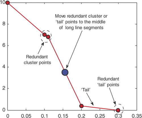
The flexible representation of the CZMs may also lead to clustering of points and the forming of a ‘tail’ (Figure 11). Apparently, in such situations, the control points are not fully utilized to help the evolution of the CZM. Therefore, it is desirable to redistribute the control points while maintaining the CZM shape. The approach we used is to remove the redundant cluster or ‘tail’ points and add additional points in the middle of longer segments as demonstrated also in Figure 11. The examination of possible clustering and a ‘tail’ is carried out for each iteration with little computational effort. Once either a ‘tail’ or a clustering is detected by certain pre-set criteria, the N–M optimization is temporarily terminated, the control points are redistributed, a new initial guess is computed and the N–M optimization is restarted. All these steps are done automatically. Demonstration of such operation and of its effect will be provided in the numerical examples presented in Section 3.3.2.

Figure 11. Illustration of redundant cluster points and ‘tail’ points possibly formed in the spline representation of CZM and the treatment.

3. Numerical examples

3.1. Direct problem

Five cases are simulated (Table 1), each of which is a combination of a particular modulus of elasticity of the bulk material and a CZM (Figure 5). Cases I–III compare the effect of different CZM shapes. Cases I, IV and V compare the effect of the bulk material stiffness.

Table 1. Five direct problem cases, combinations of CZM and modulus of elasticity.

	Case I	Case II	Case III	Case IV	Case V
CZM	Linear	HD	PL	Linear	Linear
E of bulk material (GPa)	30	30	30	10	100

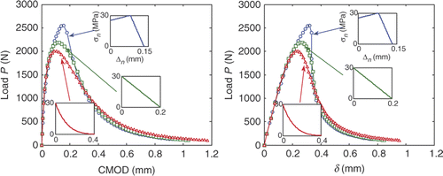
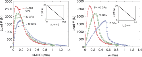
In the simulation, the loading is displacement controlled. The global responses, P versus CMOD and P versus load–line displacement δ, for cases I–III are shown in Figure 12. One can see that the CZM shape affects the global response apparently around the peak load, while for the rest of the softening curves, the curves are similar. An important implication is that numerical simulation to match most of the part of the global response curve does not prove that the right shape of CZM is used.

Figure 12. Load, P, versus load–line displacement, δ, and P versus CMOD curves for different (linear, PL and HD) CZMs, but the same bulk elastic modulus E = 30 GPa.

Figure 13 shows that the global response curves for cases I, IV and V. When E increases, the displacement variation decreases, as can be seen from the increasing deviation of P versus CMOD curve from P versus δ curve. This shows that with a fixed measurement accuracy, the relative measurement errors of displacement field for softer material will be smaller; thus the inversely computed CZM may be more accurate.

Figure 13. Load, P, versus load–line displacement, δ, and P versus CMOD curves for different bulk elastic moduli (E = 10, 30 and 100 GPa), but the same linear CZM.

The areas under the P versus δ curves divided by the area of crack surface are used to estimate the fracture energy G_f, i.e. the area under the σ versus Δ_n curve. A value comparable to the measured CMOD (0.95 CMOD in our case) is used as an estimate of Δ_nc. The target CZM to be computed is first assumed to have linear softening curve; the critical stress is then given by An initial guess of CZM, equivalently the unknown set of parameters λ, is thereby obtained.

3.2. Errors for the displacement field

Apparently, measuring CZM properties requires high precision measurement for at least the complete profile of COD, which can be part of the whole displacement field obtained by, e.g. DIC technique. However, noisy data are the real outcome of any experimental measurement. Therefore, we need to take into account the possible measurement errors in the inverse procedure to compute CZM. The nature of the errors, e.g. random or systematic, and the magnitude of the errors can be estimated from their sources. For this study, it is assumed that the displacement field is measured by DIC technique and the primary sources of errors are from the digital image resolution and the DIC algorithm. Actually, DIC is an optical technique and its resolving power depends both on the correlation algorithm and the image acquisition device. Usually, the quality of a digital image can be guaranteed with modern CCD (charge-coupled device) or CMOS (complementary metal-oxide-semiconductor) cameras. High CCD or CMOS sensor resolution, together with high magnification lenses, is able to achieve a resolution in the scale of 10⁰–10² microns pixel⁻¹. This is the base-line resolution, or maximum error, if displacement is directly obtained from the image. Resolution of DIC software is measured as a fraction of pixel. It has been reported 50 that DIC can obtain a sub-pixel precision of 0.005 pixel or even higher 51. The combined resolving power of high image resolution and high precision DIC algorithm can reach 10⁻²–10⁰ microns pixel⁻¹. The most popular DIC algorithm is based on sub-set cross-correlation; the displacements measured at all points are independent of each other. The errors can be assumed to be randomly and normally distributed.

For the inverse procedure used in this study, we introduce errors by only considering the DIC resolution since the displacement error from digital image itself never exceeds 1 pixel. Assume a moderate image resolution of 1000 pixels along the specimen height, which corresponds to 0.0255 mm pixel⁻¹. We then introduce three levels of errors by specifying different maximum error magnitudes (Table 2).

Table 2. Different levels of errors added to the synthetic displacement field.

Image resolution (mm pixel^−1)		DIC resolution (pixel)		Maximum absolute error (mm)	Estimated standard deviation or errors (mm)	Comments on the errors
0.0255	×	No error	=	0	0	Ideal
0.0255	×	0.005	=	1.28 × 10^−4	7.2–7.4 × 10^−5	Accurate
0.0255	×	0.05	=	1.28 × 10^−3	7.2–7.4 × 10^−4	Moderate
0.0255	×	0.2	=	5.1 × 10^−3	2.9–3.0 × 10^−3	Coarse

In Table 2, the case with no error serves as the control case. The standard deviation of the introduced errors is estimated based on a population of 5000 random data. The errors added are all between the interval of negative and positive maximum errors. The mean value of the errors is zero. The comments on the errors are our subjective judgement based on reported accuracy of DIC. The moderate error level is reasonable and can be easily achieved for well-control experiments.

3.3. Results of inverse analysis

The specified errors in Table 2 are added to the displacement field taken at 60% of the peak load for all five cases listed in Table 1. The weights in Equation (16), and , are taken as unit for all the examples. Due to the random nature of the errors, each case with a specified level of noise has been repeated two more times to see the variance. In all cases, four control points are used to construct the CZM. Correspondingly, there are six unknown parameters to determine in the optimization procedure. Four control points are sufficient for ‘imaginable’ CZM shape. The initial guess of the CZM is estimated from the method described in Section 3.1. LS interpolation is used for the CZM.

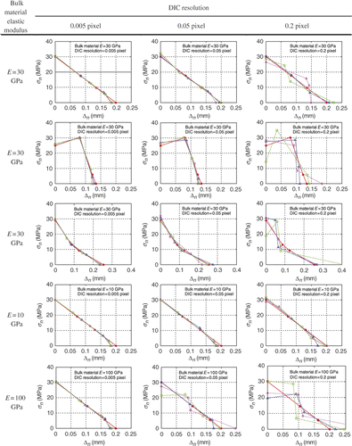
Figure 14 shows the computed CZMs for all cases with different error levels applied. The effects of the bulk material stiffness, the different CZMs and the different error levels to the computed CZMs can all be compared. The computed CZM for the case with no error added is identified in all subfigures as the solid line with solid circular markers. For the case of bulk material E = 30 GPa, the computed CZMs of all three types (linear, HD and PL) are satisfactory up to an error level = 0.05 pixel. At error level = 0.2 pixel, the computed CZMs are significantly off the exact solution. When the bulk material is E = 10 GPa, the computed CZMs are acceptable up to 0.2 pixel error level. In fact, the relative error level with respect to the absolute displacement measurement for the case of E = 10 GPa with error level = 0.2 pixel is similar to that obtained for the case of E = 30 GPa with error level = 0.05 pixel. For bulk material E = 100 GPa, apparently, the relative error is about 3.3 times that for E = 30 GPa for the same absolute error. Therefore, the bulk material with E = 100 GPa is much less tolerable to errors, as can be seen for the significant deviation of computed CZMs from the exact one when error level = 0.05 pixel.

Figure 14. Computed CZMs for all cases (Table 1) with different error levels (Table 2) applied. Each case is repeated three times. The solid circle with solid line is the computed CZM for the ideal case (without errors).

Table 3 shows the initial and final values of objective functions and the number of iterations. For cases with errors, the data are the averages of three repetitions. The table shows that as the error level increases, both the initial and the final values of objective function increase. The final objective function value does not indicate whether the computed CZM converges to the correct solution or not. For example, for the case of bulk material E = 10 GPa at error level = 0.2 pixel, the average final objective function value is 297.3, which is the largest among all cases; yet it still yields the correct CZM. For the case of bulk material E = 100 GPa at error level = 0.05 pixel, the average final objective function value is 55.6, which is moderate among all cases; but the computed CZMs are not close to the correct solution.

Table 3. Initial and finial values of objective function and number of iterations for all cases. The data for all cases with errors are the averages of three repetitions.

Bulk material elastic modulus (GPa)	Target CZM	Peak error level (DIC resolution)			No. of iterations
30	Linear	0	1562.0	1.0	408
		0.005	1647.4	34.5	307
		0.05	1656.6	55.2	342
		0.2	1732.8	149.0	250
30	HD	0	1139.4	1.6	826
		0.005	1245.3	42.1	590
		0.05	1288.2	70.1	435
		0.2	1331.2	147.3	390
30	PL	0	2413.9	5.5	522
		0.005	2535.1	31.1	349
		0.05	2546.6	47.1	293
		0.2	2601.8	154.0	242
10	Linear	0	2340.8	0.8	261
		0.005	2425.1	82.7	365
		0.05	2461.5	99.5	364
		0.2	2685.4	297.3	240
100	Linear	0	926.4	0.7	422
		0.005	988.9	19.8	346
		0.05	1054.1	55.6	283
		0.2	1009.2	170.3	214
Note: λ^(0) is initial guess and λ^(^n^) is the converged result. The convergent criterion is set as .

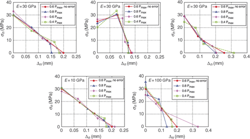
3.3.1. Displacement data at different load levels

At high error levels, each individual inverse analysis converges to an inaccurate CZM. Using a few data sets of the same case enhances the estimation of the computed CZM. For example, one would naturally choose to estimate the CZM using all three repetitions for cases of bulk material E = 30 GPa at error level = 0.2 pixel or bulk material E = 100 GPa at error level > 0.05 pixel shown in Figure 14. In practice, this can be done by taking several DIC measurements at the same loading and using the average of the computed CZM from each measurement. Another way, which may be more preferable and may give more confidence, is to use the DIC measurement at several loadings. As a demonstration, we use the displacement field taken at 40%, 60% and 80% of the peak load at post-peak regime. All five cases (Table 1) are applied at an error level = 0.1 pixel. Figure 15 shows the final result. As shown in Figure 15, the exact CZM is close to the average of the computed CZMs from displacement data with errors, even for the case of bulk material E = 100 GPa.

Figure 15. CZMs computed using displacement field taken at different post-peak loadings. An error level = 0.1 pixel is applied to all cases.

3.3.2. Other numerical aspects

Some other features of the proposed optimization scheme are: (1) the initial guess of CZM for the optimization; (2) the number of control points defining the CZM; (3) the interpolation used for constructing the CZM and (4) the aid to optimization. In previous sections, the presented results are all determined using four control points and LSs as interpolant; the initial guesses of the CZM are all estimated by using P versus δ curve, which is not far from the exact solution. For a further demonstration of the effectiveness of the proposed inverse procedure, four cases are presented (corresponding to different initial guesses) as outlined in Table 4. For these four cases, we use six control points to illustrate the more flexible shape representation, although this is more than enough for the current need. There are only three relative relations of CZM curves between the initial guess and the exact solution: (1) intersecting, which is the case for all previously presented cases; (2) below (Figure 16a) and (3) above (Figure 16b). The initial guesses and the computed converged CZMs for these four cases are shown in Figure 16.

Figure 16. Illustration of optimization effectiveness for (1) different initial guesses: below and above the solution; (2) higher number of control points: six here; and (3) different interpolations: linear and cubic spline interpolations. Left: for HD CZM. Right: for PL CZM.

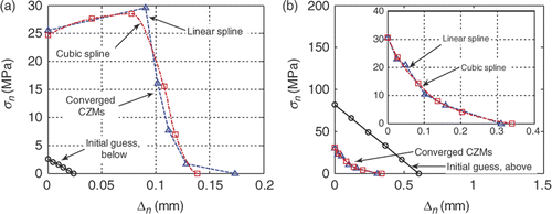
Table 4. Effect of the initial guess (six control points), and use of different interpolants.

Cases	Target CZM	Bulk material, E (GPa)	Number of control points	Initial guess	Interpolant
I	HD	30	6	Below	LS
II	HD	30	6	Below	Cubic spline
III	PL	30	6	Above	LS
IV	PL	30	6	Above	Cubic spline

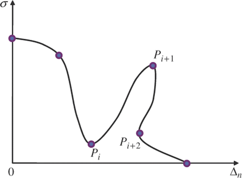
Notice that in Figure 16a, the computed HD CZM using LS interpolations is not exact due to a small ‘tail’ present in the solution, which is not removed during optimization. However, as can be seen, the computed HD CZMs using both interpolants are fairly accurate. For the PL CZM, both interpolants yield accurate CZMs. A close examination of the curve confirms the expectation that the cubic spline interpolations provide smoother and more accurate results. The evolution of the objective function value for these four cases is presented in Figure 17. In each plot shown in Figure 17, the locations where clustering or ‘tail’ forms, as described in Section 2.2.6, are marked in one of the two curves. The initial objective function values for these four cases are much larger than those shown in Table 3. Also, the number of iterations to convergence is much larger. The objective function values steadily decrease except at ‘tail’ points when the CZM parameters are recalculated. Although the cohesive stress contributed by the ‘tail’ is small, it is located away from the beam neutral axis. With a long moment arm, the influence of the ‘tail’ to the deformation of the specimen is apparent. The treatment of the clustered points may only influence the objective function negligibly, as seen closely at point ‘C’ on the right plot of Figure 17.

Figure 17. The evolution of the objective function value for the four cases shown in Figure 16. Upper plot: for HD CZM. Lower plot: for PL CZM.

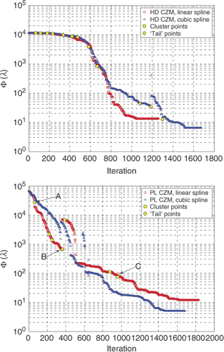
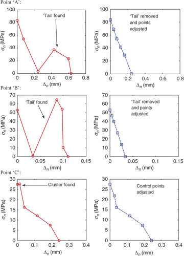
Figure 18 shows the adjustment of control points for the two ‘tails’ found at points ‘A’ and ‘B’ and for the clustering found at point ‘C’ in Figure 17. The removal of the ‘tail’ at point ‘A’ does not affect the objective function value as the ‘tail’ corresponds to crack opening larger than the actual case. At point ‘B’, the cohesive stress within the tail acts on the specimen thus affecting the deformation and the value of the objective function. The treatment of the clustering, as illustrated, does not change the CZM curve significantly, and therefore does not influence the objective function value much. A comparison between cases with and without cluster removal shows that the cluster treatment reduces the number of iterations significantly.

Figure 18. Demonstration of the removal of ‘tail’ or cluster formed in the CZM representation. Points ‘A’–‘C’ correspond to the points shown in Figure 17.

3.3.3. Remarks on the uniqueness of the inverse solutions

In general, inverse problems may not have unique solutions in a feasible domain. In optimization description, this means there may exist a finite or infinite number of local minimums in the feasible domain. The solution is usually one of these local minimums and may not be the global minimum. Therefore, it is important to clearly identify the local minimum that is physically representative. In this application, it seems that the unwanted local minimums are mostly induced by the CZM ‘tail’. Point ‘B’ in Figure 18 in fact leads to a local minimum if the tail is not removed, as removal of the ‘tail’ causes an increase of the objective function value (Figure 17). As one can imagine, if the ‘tail’ is totally to the right of the actual maximum COD, the cohesive stress due to the ‘tail’ will not contribute to the deformation of the specimen, i.e. the existence of the ‘tail’ will not affect the objective function value. Apparently, one does not expect a CZM to have a ‘tail’ like the ones shown in Figure 18. In practice, this probably is not an issue as the CZM will be computed from different sets of experimental data, e.g. at different load levels (Figure 15), or from specimens with different geometries (either numerical or actual experimental specimens).

4. Conclusions

In this article, a method is proposed to compute the CZM from whole-field displacement data. The major differences between this method and previous methods are: (1) a whole displacement field is used rather than curve fitting using global response, (2) no specific shape is assumed for CZM during inverse computation and (3) no derivatives of a synthetic (or experimental) displacement field are needed.

Linear and cubic splines are used to represent the shape of the CZM. The advantage brought by splines is the flexibility of using an arbitrary number of control points for representing an arbitrary shape. The non-linear inverse problem is solved using the unconstrained, derivative-free optimization method, the N–M method. The objective function is taken to be the difference between the measured displacement field and the computed displacement field from FEM, but augmented by adding continuous barrier functions to suppress the non-physical compressive cohesive stress and snapback of the CZM curve during optimization. The barrier functions enforce the requirement of using the unconstrained unknown parameters in the N–M method as long as the initial guess for the optimization problem is within the feasible domain.

The numerical examples investigate cases with different moduli of elasticity of the bulk material, different CZMs and different levels of errors (corresponding to potential noise in the experimental data). The numerical examples have shown that the proposed scheme is quite tolerant to experimental errors but the accuracy of the computed CZM heavily depends on the elastic modulus of the bulk material. The robustness and effectiveness of the proposed scheme are also demonstrated using different initial guesses and a different number of control points.

Acknowledgement

This study was supported by the National Science Foundation under the Partnership for Advancing Technology in Housing program (NSF-PATH Award no. 0333576).

Appendix

Nomenclature

u	=	displacement field, also global displacement vector;
	=	known displacement field from direct problem or from experimental measurement;
u*	=	computed displacement field during inverse procedure;
λ	=	CZM parameters;
σ	=	cohesive stress/traction;
σc	=	critical cohesive stress;
Δn	=	COD;
Δnc	=	critical COD;
γ	=	PL softening index;
	=	bulk element stiffness matrix;
	=	element cohesive stiffness matrix;
Kb	=	global stiffness matrix of the bulk material;
Kc	=	global cohesive stiffness matrix;
ue	=	element nodal displacement;
r	=	element nodal force;
l	=	size of Q4 element along crack surface;
s	=	local natural coordinate;
t	=	beam thickness;
kc	=	defined as σ/Δn;
Ns	=	shape function in natural coordinate system;
N	=	shape function in isoparametric coordinate system;
ux	=	element nodal displacement in x direction;
Fext,	=	global external force;
Δn, σ	=	coordinates of the control points;
R	=	residual of the FE system of equations;
θb, Nb, ξi	=	parameters that define the barrier functions;
wu	=	vector of weighting factors;
μ	=	number of internal control points;
M	=	number of unknown parameters of the CZM;
Φ(λ)	=	objective function;
Gf	=	fracture energy;
β1, β2	=	barrier functions;
	=	weighting factors for the barrier functions.

References

- Barenblatt, GI, 1959. The formation of equilibrium cracks during brittle fracture: General ideas and hypotheses. Axially-symmetric cracks, J. Appl. Math. Mech. 23 (1959), pp. 622–636.
- Dugdale, DS, 1960. Yielding of steel sheets containing slits, J. Mech. Phys. Solids 8 (1960), pp. 100–104.
- Hillerborg, A, Modéer, M, and Petersson, PE, 1976. Analysis of crack formation and crack growth in concrete by means of fracture mechanics and finite elements, Cem. Concr. Res. 6 (1976), pp. 773–781.
- Xu, XP, and Needleman, A, 1994. Numerical simulations of fast crack growth in brittle solids, J. Mech. Phys. Solids 42 (1994), pp. 1397–1434.
- Zhang, Z, and Paulino, GH, 2005. Cohesive zone modeling of dynamic failure in homogeneous and functionally graded materials, Int. J. Plast. 21 (2005), pp. 1195–1254.
- Camacho, GT, and Ortiz, M, 1996. Computational modeling of impact damage in brittle materials, Int. J. Solids Struct. 33 (1996), pp. 2899–2938.
- Ortiz, M, and Pandolfi, A, 1999. Finite-deformation irreversible cohesive elements for three-dimensional crack-propagation analysis, Int. J. Numer. Methods Eng. 44 (1999), pp. 1267–1282.
- Zhang, Z, and Paulino, GH, 2007. Wave propagation and dynamic analysis of smoothly graded heterogeneous continua using graded finite elements, Int. J. Solids Struct. 44 (2007), pp. 3601–3626.
- Moes, N, and Belytschko, T, 2002. Extended finite element method for cohesive crack growth, Eng. Fract. Mech. 69 (2002), pp. 813–833.
- Wells, GN, and Sluys, LJ, 2001. A new method for modeling cohesive cracks using finite elements, Int. J. Numer. Methods Eng. 50 (2001), pp. 2667–2682.
- Rahulkumar, P, 2000. Cohesive element modeling of viscoelastic fracture: Application to peel testing of polymers, Int. J. Solids Struct. 37 (2000), pp. 1873–1897.
- Zhang, Z, Paulino, GH, and Celes, W, 2007. Extrinsic cohesive modeling of dynamic fracture and microbranching instability in brittle materials, Int. J. Numer. Methods Eng. 72 (2007), pp. 893–923.
- Roesler, J, Paulino, GH, Park, K, and Gaedicke, C, 2007. Concrete fracture prediction using bilinear softening, Cem. Concr. Compos. 29 (2007), pp. 300–312.
- Shim, D-J, Paulino, GH, and Dodds, RH, 2006. J resistance behavior in functionally graded materials using cohesive zone and modified boundary layer models, Int. J. Fract. 139 (2006), pp. 91–117.
- Song, SH, Paulino, GH, and Buttlar, WG, 2006. Simulation of crack propagation in asphalt concrete using an intrinsic cohesive zone model, ASCE J. Eng. Mech. 132 (2006), pp. 1215–1223.
- Song, SH, Paulino, GH, and Buttlar, WG, 2008. "Influence of the cohesive zone model shape parameter on asphalt concrete fracture behavior". In: Paulino, GH, Pindera, M-J, Dodds, RH, Rochinha, FA, Dave, EV, and Chen, L, eds. Multiscale and Functionally Graded Materials, AIP Conference Proceedings 973. 2008. pp. 730–735.
- van Mier, JGM, and van Vliet, MRA, 2002. Uniaxial tension test for the determination of fracture parameters of concrete: State of the art, Fract. Concrete Rock 69 (2002), pp. 235–247.
- Yang, J, and Fischer, G, 2006. "Simulation of the tensile stress-strain behavior of strain hardening cementitious composites". In: Konsta-Gdoutos, MS, ed. Measuring, Monitoring and Modeling Concrete Properties. Springer: Dordrecht; 2006. pp. 25–31.
- Shah, SP, Ouyang, C, and Swartz, SE, 1995. Fracture Mechanics of Concrete: Applications of Fracture Mechanics to Concrete, Rock and other Quasi-brittle Materials. New York: Wiley; 1995.
- Volokh, KY, 2004. Comparison between cohesive zone models, Commun. Numer. Methods Eng. 20 (2004), pp. 845–856.
- Bolzon, G, Fedele, R, and Maier, G, 2002. Parameter identification of a cohesive crack model by Kalman filter, Comput. Methods Appl. Mech. Eng. 191 (2002), pp. 2847–2871.
- Maier, G, Bocciarelli, M, Bolzon, G, and Fedele, R, 2006. Inverse analyses in fracture mechanics, Int. J. Fract. 138 (2006), pp. 47–73.
- Que, NS, and Tin-Loi, F, 2002. Numerical evaluation of cohesive fracture parameters from a wedge splitting test, Eng. Fract. Mech. 69 (2002), pp. 1269–1286.
- Que, NS, and Tin-Loi, F, 2002. An optimization approach for indirect identification of cohesive crack properties, Comput. Struct. 80 (2002), pp. 1383–1392.
- Tin-Loi, F, and Que, NS, 2002. Nonlinear programming approaches for an inverse problem in quasibrittle fracture, Int. J. Mech. Sci. 44 (2002), pp. 843–858.
- van Mier, JGM, 1997. Fracture Processes of Concrete: Assessment of Material Parameters for Fracture Models. Boca Raton: CRC Press; 1997.
- Elices, M, 2002. The cohesive zone model: Advantages, limitations and challenges, Eng. Fract. Mech. 69 (2002), pp. 137–163.
- Seong Hyeok, S, Paulino, GH, and Buttlar, WG, 2006. A bilinear cohesive zone model tailored for fracture of asphalt concrete considering viscoelastic bulk material, Eng. Fract. Mech. 73 (2006), pp. 2829–2848.
- Song, SH, Paulino, GH, and Buttlar, WG, 2005. Cohesive zone simulation of mode I and mixed-mode crack propagation in asphalt concrete. Geo-Frontiers 2005. Reston, VA, Austin, TX, USA: ASCE; 2005. pp. 189–198.
- Dally, JW, and Riley, WF, 2005. Experimental Stress Analysis. Knoxville, Tenn: College House Enterprises; 2005.
- Bonnet, M, and Constantinescu, A, 2005. Inverse problems in elasticity, Inverse Prob. 21 (2005), pp. 1–50.
- Avril, S, Bonnet, M, Bretelle, A-S, Grediac, M, Hild, F, Ienny, P, Latourte, F, Lemosse, D, Pagano, S, Pagnacco, E, and Pierron, F, 2008. Overview of identification methods of mechanical parameters based on full-field measurements, Exp. Mech. 48 (2008), pp. 381–402.
- Abanto-Bueno, J, and Lambros, J, 2002. Investigation of crack growth in functionally graded materials using digital image correlation, Eng. Fract. Mech. 69 (2002), pp. 1695–1711.
- Abanto-Bueno, J, and Lambros, J, 2005. Experimental determination of cohesive failure properties of a photodegradable copolymer, Exp. Mech. 45 (2005), pp. 144–152.
- Tan, H, Liu, C, Huang, Y, and Geubelle, PH, 2005. The cohesive law for the particle/matrix interfaces in high explosives, J. Mech. Phys. Solids 53 (2005), pp. 1892–1917.
- Geymonat, G, and Pagano, S, 2003. Identification of mechanical properties by displacement field measurement: A variational approach, Meccanica 38 (2003), pp. 535–545.
- Roux, S, and Hild, F, 2008. Digital image mechanical identification (DIMI), Exp. Mech. 48 (2008), pp. 495–508.
- Genovese, K, Lamberti, L, and Pappalettere, C, 2005. Improved global-local simulated annealing formulation for solving non-smooth engineering optimization problems, Int. J. Solids Struct. 42 (2005), pp. 203–237.
- Molimard, J, Le Riche, R, Vautrin, A, and Lee, JR, 2005. Identification of the four orthotropic plate stiffnesses using a single open-hole tensile test, Exp. Mech. 45 (2005), pp. 404–411.
- Grediac, M, Pierron, F, Avril, S, and Toussaint, E, 2006. The virtual fields method for extracting constitutive parameters from full-field measurements: A review, Strain 42 (2006), pp. 233–253.
- Avril, S, and Pierron, F, 2007. General framework for the identification of constitutive parameters from full-field measurements in linear elasticity, Int. J. Solids Struct. 44 (2007), pp. 4978–5002.
- Song, SH, Paulino, GH, and Buttlar, WG, 2006. Simulation of crack propagation in asphalt concrete using an intrinsic cohesive zone model, J. Eng. Mech. 132 (2006), pp. 1215–1223.
- Dick-Nielsen, L, Stang, H, and Poulsen, PN, 2006. "Condition for strain-hardening in ECC uniaxial test specimen". In: Konsta-Gdoutos, MS, ed. Measuring, Monitoring and Modeling Concrete Properties. Springer: Dordrecht; 2006. pp. 41–47.
- De Boor, C, 2001. A Practical Guide to Splines. New York: Springer; 2001.
- Deuflhard, P, and Hohmann, A, 2003. Numerical Analysis in Modern Scientific Computing: An Introduction. New York: Springer; 2003.
- Fletcher, R, 1987. Practical Methods of Optimization. Chichester; New York: Wiley; 1987.
- Nelder, JA, and Mead, R, 1965. Simplex method for function minimization, Comput. J. 7 (1965), pp. 308–313.
- Nocedal, J, and Wright, SJ, 2006. Numerical Optimization. New York: Springer; 2006.
- Bezerra, LM, and Saigal, S, 1993. A boundary element formulation for the inverse elastostatics problem (IESP) of flaw detection, Int. J. Numer. Methods Eng. 36 (1993), pp. 2189–2202.
- Lu, H, and Cary, PD, 2000. Deformation measurements by digital image correlation: Implementation of a second-order displacement gradient, Exp. Mech. 40 (2000), pp. 393–400.
- Cheng, P, Sutton, MA, Schreier, HW, and McNeill, SR, 2002. Full-field speckle pattern image correlation with B-spline deformation function, Exp. Mech. 42 (2002), pp. 344–352.