Application of transient experimental techniques for developing a heat transfer correlation for mixed convection in porous medium

Abstract

An approach based on transient heat transfer experiments combined with numerical optimization procedures is studied to develop a heat transfer correlation for mixed convection heat transfer in a vertical duct filled with metallic porous structures. The heat source of the vertical duct is a near isothermal plate which during cooling is treated as a lumped heat capacity model. The temperature–time history, during the cooling of the plate, is measured using K-type (36AWG) thermocouples connected to a PC-based data acquisition system. A numerically computed temperature–time history of the plate is then compared with the experimentally known temperature–time history to estimate the residual. The minimization of sum of the squares of the residual is done using a hybrid numerical optimization technique, i.e. a combination of Genetic Algorithm and the Levenberg–Marquardt method, in order to obtain the coefficient and the exponents of the pertinent non-dimensional parameters in the Nusselt number correlation. The consistency of the present approach is further substantiated by comparing the Nusselt number values predicted using the proposed correlation and that evaluated from the steady-state experiments.

Keywords:

• transient experiment
• lumped heat capacity model
• parameter estimation
• hybrid optimization
• steady-state experiment

Nomenclature

As	=	surface area of the hot wall (m2)
a	=	coefficient (parameter) in the Nusselt number correlation to be estimated
b	=	exponent (parameter) of modified Grashof number, in the Nusselt number correlation, to be estimated
Cp	=	specific heat of the material of the hot plate (J kg−1 K−1)
c	=	exponent (parameter) of Peclet number, in the Nusselt number correlation, to be estimated
Da	=	Darcy number
Dh	=	hydraulic diameter of the channel (m)
F	=	difference between the measured and numerically computed data
GrD	=	Grashof number based on hydraulic diameter,
	=	modified Grashof number, defined in Equation (6)
g	=	gravitational acceleration, 9.81 (m s−2)
h	=	average heat transfer coefficient (W m−2 K−1)
I	=	Identity matrix
J	=	Jacobian matrix
K	=	permeability of the porous medium (m2)
kf	=	thermal conductivity of fluid (air) (W m−1 K−1)
km	=	effective thermal conductivity of the porous medium (W m−1 K−1)
ks	=	thermal conductivity of solid (brass) (W m−1 K−1)
m	=	mass of the hot plate (kg)
	=	average convective Nusselt number
Pe	=	Peclet number
Q	=	dependent variable in the uncertainty analysis
QL	=	unaccountable heat losses (W)
qw	=	heat flux at the wall (W m−2)
R	=	sum of the squares of the error between the measured and computed temperature–time data
ReD	=	Reynolds number based on the hydraulic diameter
T	=	temperature (K)
Tf	=	film temperature (K)
ΔTavg	=	average wall temperature excess with respect to fluid-free stream temperature (K)
t	=	time (s)
U	=	fluid free steam velocity (ms−1)
X	=	transpose of the vector of unknown parameters ‘a, b and c’
x	=	Cartesian co-ordinate (m)
	=	Greek symbols
α	=	thermal diffusivity of fluid (m2 s−1)
αm	=	effective thermal diffusivity of porous medium (m2 s−1)
β	=	isobaric cubic expansivity of fluid (K−1)
∞	=	free stream
λ	=	damping parameter
μ	=	dynamic viscosity of fluid (N s m−2)
ν	=	kinematic viscosity of fluid (m2 s−1)
ω	=	random number
ϕ	=	porosity of porous material
ρ	=	density of fluid (kg m−3)
σ	=	standard deviation (SD) of random errors
	=	Subscripts
f	=	fluid
h	=	hot
in	=	inlet
int	=	initial
w	=	wall/plate
	=	Superscripts
exp	=	experimental
meas	=	measured
num	=	numerical

1. Introduction

Parameter estimation problems are invariably posed as optimization problems, wherein a residual is usually minimized. In inverse thermal problems, parameter estimation is done by minimizing an objective function which is usually defined as the sum of the squares of error (residual) between known/measured and estimated/simulated data. The estimated data or the simulated data are obtained by solving the mathematical model representing the heat transfer problem. In this study the parameters of interest, i.e. the coefficient and the exponents of non-dimensional parameters in the Nusselt number correlation, need to be estimated from the measured temperature–time history of a lumped capacity heat transfer model during cooling. The mathematical model of transient cooling of a lumped heat capacity model is solved for assumed values of the parameters of interest to obtain the simulated temperature–time history. The objective function is then defined as the sum of the squares of the error (residual) between measured and simulated temperature–time history. In this study, the minimization of the sum of the squares of the residual is done using a hybrid numerical optimization technique, i.e. a combination of genetic algorithm (GA) and the Levenberg–Marquardt method, in order to obtain the coefficient and the exponents of the pertinent non-dimensional parameters in the Nusselt number correlation.

Near-porous medium models prepared from different kinds of solid matrices have been considered as a promising option for heat transfer enhancement application from thermally loaded surfaces. Because of random structures of porous media, they are different in geometry and physical and thermal properties. Consequently, the flow and heat transfer characteristics in these media also differ significantly. Megerlin et al. 1 experimentally demonstrated the use of mesh and brush inserts to enhance heat transfer in electrically heated circular tube test sections. The authors reported that the use of mesh inserts in tubes increases the heat transfer coefficient about nine times in comparison with empty tubes for the same mass velocities and for the case with brush inserts the improvement in the heat transfer coefficient was about five times. Renken and Poulikakos 2 investigated, experimentally and numerically, forced convective heat transport in a packed bed of spheres occupying a parallel plate channel whose walls are maintained at constant temperatures. Calmidi and Mahajan 3 carried out experimental and numerical studies to investigate forced convection in horizontal channel embedded with high-porosity metal foams with due attention given to understanding the thermal dispersion and thermal non-equilibrium effects in metal foams. Pavel and Mohamad 4 investigated, experimentally, the potential of metallic porous materials, manufactured from aluminium screens, in enhancing forced convective heat transfer from a pipe subjected to a constant and uniform heat flux. The results showed that higher heat transfer rates using porous inserts can be achieved at the expense of a reasonable pressure drop. Raju and Narasimhan 5, using a numerical study, presented a novel approach of treating near-compact heat exchangers (in-line tube-to-tube arrangement) as global porous media for estimating the global thermo-hydraulic characteristics. The authors presented correlations for non-dimensional pressure drop and Nusselt number for characterizing the thermo-hydraulic performance of the chosen near-compact heat exchanger configurations.

Studies on heat transfer in porous media filled in vertical channel/annulus are limited. Pu et al. 6 experimentally investigated mixed convection in a vertical channel packed with chrome steel spheres and heated asymmetrically. From the experimental observations, the transition regime from natural to forced convection limits was proposed for the geometry considered in their study. Reda 7 studied, experimentally and numerically, mixed convection in a vertical annulus packed with glass spheres and obtained the radial temperature profiles in the bed. Choi and Kulacki 8 performed both experimental and numerical investigations on mixed convection through vertical porous annuli locally heated from the inner cylinder. Based on numerical results, the Nusselt numbers were correlated by the parameter groups and , and the regressed form of Nusselt number was then compared with the experimentally measured Nusselt number.

The review of literature reveals that most of the previous studies have restricted their attention to metallic porous materials inserted in horizontal channels and studies with metallic porous structures inserted in vertical rectangular channels are scarce. Also, the porous media that have been employed in the vertical channel/annuli were made of conventional granular beads. Furthermore, the heat transfer correlations reported in earlier studies for estimating the heat transfer rates are the outcome of steady state analysis only. This study, however, reports the applicability of transient experimental technique to evolve a Nusselt number correlation for mixed convection heat transfer in a vertical duct filled with metallic porous structures made from a stack of metallic perforated sheets.

2. Experimental setup

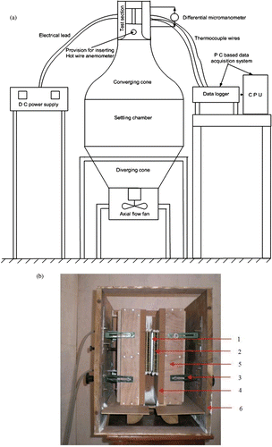
The experiment setup composed of a vertical duct, porous media and a plate-heater assembly is built inside the test section of a vertical wind tunnel. The vertical duct of dimensions 390 mm× 250 mm × 62 mm is made of 25 mm thick non-rubberized cork supported by wooden boxes made of 12 mm plywood panel. The wooden boxes are fixed to the side walls of the test section of the wind tunnel using ‘L’-shaped mild steel brackets, two on each side of the wooden boxes. The grooves made on the brackets facilitate movement of the walls of the duct along the three coordinate directions and therefore allow the wooden boxes to be fixed at any desired position by means of locking nuts. A nut-and-screw arrangement, one at the bottom and the other at the top, on the back side of each wooden box permits the walls of the duct to move away from or closer to both vertical centre axes of the test section. Such an arrangement helps in keeping and aligning the porous media and the heater-plate assembly in position thereby maintaining the dimensional accuracy of the test section. Furthermore, the non-rubberized cork used for constructing the walls of the duct, due to its cushioning effect, ensures an air-tight test section after all locking nuts are tightened properly. A bell mouth is constructed at the entrance to the vertical duct to minimize the entry losses, thereby ensuring a uniform flow at the inlet of the test section. A schematic diagram of the experimental setup and a photograph of the test section are shown in Figure 1(a) and (b), respectively.

Figure 1. (a) Schematic representation of the experimental setup used for the mixed convection study in a channel filled with porous medium (b) Photograph of the experimental setup (one end wall is in removed position). 1. Plate heater assembly. 2. Porous medium. 3. L-clamp. 4. Non-rubberized cork. 5. Wooden box. 6. Side walls of test section of wind tunnel.

The plate-heater assembly essentially consists of two aluminium plates of dimensions 150 × 250 × 3 mm with a flat heater sandwiched between them. The flat heater is formed by winding a Nichrome wire over a mica sheet and the heater is electrically insulated from the unexposed side of the aluminium plates by using thin mica foils. Ten ‘K-type’ (36AWG) stainless steel sheathed thermocouples, five on each aluminium plate, are used for the measurement of temperatures at several locations of the heated plate. They are fixed to the plates using copper cement that has a high thermal conductivity. All thermocouples are calibrated before fixing them into the grooves machined in the plates and the maximum measurement error is within ±0.2°C. The thermocouples are connected to a PC-based data acquisition system (Model No. 34970A, Agilent Technologies Ltd.) through compensating wires. The power input to the heater is supplied from a regulated DC power source which has a range of 30–600 V and 0–1.5 A.

The metallic porous structures used for the experiments are prepared from the commercially available 1.5 mm thick perforated brass sheets having stamped holes of 3 mm diameter. Initially, a large number of perforated sheets with slightly larger dimensions than 250 mm × 27 mm are cut from large perforated ones and a group of such cut-sheets are then given a soft grinding operation to achieve the desired dimensions, i.e., 250 × 27 × 1.5 mm. After the grinding operation, the edges of each sheet are rubbed with emery paper to remove any burr that would occur during the grinding operation. The perforated sheets are then assembled together by means of washers (1 mm thick) arranged between the perforated sheets and threaded copper rods (3 mm ϕ) with fastening nuts positioned at the four corners of the perforated sheets. The perforated plates are assembled in such a way that the holes in the consecutive plates are in staggered fashion so that more residence time and thorough mixing of the fluid as it flows through the porous structure are assured. The space between the perforated sheets can be adjusted by adding or removing the washers between them and in this way porous samples of different porosities are obtained. It is worth mentioning that equal numbers of washers are used between successive perforated sheets to obtain a porous sample of desired porosity. Three different porous samples of porosity (ϕ = 0.85, 0.89 and 0.92) are prepared for which the numbers of perforated sheets used are 55, 37 and 23, respectively. The test section inside the vertical duct is made by fixing two identical porous samples, one on either side of the plate-heater assembly. The resulting physical dimensions of the vertical rectangular duct embedded with porous samples are 150 × 250 × 27 mm³, with one of the vertical walls heated and the others being adiabatic.

The commercially available perforated brass plates, used for the preparation of metallic porous structures, are examined for their metallurgical composition using a Scanning Electron Microscope (Make: FEI-Czech Republic, Model-QUANTA 200). The results of micro analysis show that the metallurgical composition of the tested specimens are Cu-K (57.34 wt%), Zn-K (31.49 wt%), C-K (8.80 wt%) and O-K (2.37 wt%). Since the metallurgical composition of the tested specimens is close to a copper-based alloy with Cu (60%) and Zn (40%), for the present experimental investigations the thermal conductivity of the solid material of the porous samples, k_s is chosen as 123 Wm⁻¹ K⁻¹ which corresponds to the thermal conductivity of brass with Cu (60%) and Zn (40%) 9. The effective thermal conductivity of the porous structures is then calculated as the weighted geometric mean of k_f and k_s, defined as in 10 (1)

The velocity and temperature of the air at the inlet of the test section are measured using a thermal anemometer (Airflow^™ TA5) and are referred to as free-steam velocity and free-stream temperature, respectively. The fluid temperature at the downstream of the test section is recorded by three K-type stainless steel sheathed thermocouples located just above the test section. Among the three thermocouples, two are located just above the porous sample placed on one side of the plate-heater assembly and the third thermocouple is located above the porous sample placed on the other side of the plate-heater assembly. It is observed that the maximum temperature variation among the three thermocouples is within ±0.6°C and this indicates that symmetry prevails about the vertical axis of the test section. A comparison of fluid enthalpy rise with the electric power input shows that the maximum heat loss from the test section is less than 6% for the power input ranging from 10 to 105 W.

2.1. Experimental procedure

The axial flow fan is switched on and its speed is adjusted using an electronic control panel to obtain the desired flow velocity at the inlet of the test section. After the flow is stabilized, the velocity and temperature of the air at the inlet of the test section are measured. The electrical energy is then allowed to flow into the plate-heater assembly at an appropriately chosen rate to heat the test section and the electrical power is switched off after steady-state conditions are reached. Steady state is deemed to be reached when the temperature of the heated wall is observed to vary within ±0.1°C in 10 min. The transient response of the wall during its cooling is recorded using the PC-based data acquisition system and this is done at regular intervals of 30 s till the wall reaches a temperature 4°C above the free stream temperature. The thermocouple that indicates the temperature close to the average temperature of the wall is chosen for recording the transient response of the system. Using an arrangement for traversing the anemometer, the velocity measurement is done at 10 different locations upstream of the test section and the mean value of the velocities is used for calculations. The experiments are repeated for several initial temperatures of the wall and different flow velocities at the inlet of the test section. The air velocity is varied by varying the speed of the axial flow fan mounted appropriately below the diffuser entry. The thermophysical property values for air are estimated at the film temperature, T_f, defined as (2)

3. Mathematical modelling

The mathematical model of transient cooling of a heat transfer model, which is idealized as a lumped heat capacity system, is given by (3)

The term, Q_L, which stands for unaccountable heat losses including heat loss by radiation, is not taken into consideration in the analysis as it is expected to be small when compared to heat loss by convection. The average convective heat transfer coefficient is replaced with the average Nusselt number correlation of the form (4)

With this, Equation (3) takes the form (5)

In Equation (5), the modified Grashof number is calculated using the following relation (6) where Darcy number, Da is defined as (7) and the Peclet number is computed as (8) where α_m denotes the effective thermal diffusivity of the porous medium and this is given by (9)

The objective now is to retrieve the parameters ‘a’, ‘b’ and ‘c’ shown in the Equation (4) from the measured temperature–time data obtained while cooling the plate.

3.1. Forward problem

Equation (5) can be rewritten as (10)

Equation (10) is the mathematical model representing the forward problem. This first order initial value problem is solved by sixth order Runge–Kutta method for the numerical computation of the temperature–time data for all known values of the system parameters and guess values of the parameters ‘a’, ‘b’ and ‘c’, subject to the initial condition T_h = T_int at t = 0.

3.2. Inverse problem

The inverse problem is posed as a parameter estimation problem wherein the sum of the squares of the error between the measured temperature–time data, () and numerically computed temperature–time data, () is minimized. The sum of the squared error is then defined as (11) where R(X) is the objective function in the optimization procedure and is minimized with respect to the elements of the unknown vector, using a hybrid optimization technique, i.e. a combination of GA and the Levenberg–Marquardt algorithm (LMA).

3.3. Solution of inverse problem by hybridization of GA with LMA

Numerical optimization algorithms based on gradient and stochastic methods are invariably used to minimize the errors between measured and estimated data. As the gradient-based methods use the information about the behaviour of a function by searching along the gradient direction, they are usually faster in their convergence and ensure high level of accuracy in the estimated values at the optimum point. In this way, gradient-based techniques are attractive from a computational point of view. However, when local type inversion algorithms are adopted, accurate and reliable results can be obtained only if the starting trial solution is close enough to the actual solutions. Convergence of global optimization techniques in general is not dependent on the guess values. However, stochastic methods generally present a low convergence rate and require a large number of cost function evaluations to achieve a satisfactory convergence threshold. Consequently, they are computationally expensive especially when compared to gradient-based optimization techniques. An effective way of improving the convergence rate and reducing the computational time simultaneously is the hybridization of stochastic methods with gradient-based technique, aiming at fully utilizing the complementary advantages of gradient-based and stochastic techniques. The simplest way to implement a hybridized version of a stochastic method is that of considering a two-stage optimization 11. In such a hybrid approach, the stochastic method is run for a small number of generations or iterations, requiring therefore a much smaller number of function evaluations. The solution obtained from the stochastic method is then used as the initial guess for the gradient-based methods. In this study, the hybridization of a GA with LMA is implemented to estimate the optimum values of the parameters pertinent to the problem considered here. Initially, a GA is used to perform a preliminary search in the solution space and to locate the neighbourhood of the solution. Then, using the best solution found with the GA as the initial guess, the Levenberg–Marquardt method is implemented to refine and improve the current solution and quickly converge towards the optimum.

3.3.1. Genetic algorithms

GAs are procedures based on mechanics of genetics and natural selection that were originally developed by Holland 12 and were popularized by Goldberg 13. GAs mimic genetic recombination and evolution in nature to solve optimization problems. They operate on a randomly generated population in the search space simultaneously and perform a global optimization by the three genetic operations, i.e. selection, crossover and mutation. According to the evolutionary theory, only the most suited elements of a population can survive and generate offsprings, thereby transmitting their biological heredity to new generations. The evolution starts from an initial population of completely random individuals represented in binary strings of 0's and 1's and involved in the generation process. The binary representation allows the implementation of binary operations such as crossover, mutation and inversion. In each generation, the fitness of the whole population is evaluated, the best or fittest models (individuals) are stochastically selected from the current population and then operations such as crossover and mutation are applied in order to combine the most successful characteristics of each model to produce a new population. The new population is then used in the next iteration of the algorithm. The suitability or the selection of each model to produce new population, according to the problem under consideration, is evaluated via a fitness value directly derived from the objective function. As GAs are derivative-free algorithms, they are capable of finding the global optimum even in the presence of local optima, noise and discontinuities. Moreover, GAs can handle both discrete and continuous variables. These generic features of GAs make them well-suited to locate the global minimum of non-linear inverse problems in engineering. The GA begins, like any other optimization algorithm, by defining the objective function, optimization variables and the search space for the variables. It ends like other optimization algorithms too, by testing for convergence. Detailed discussions of GAs can be seen in several references (see, e.g. 13–15). Since the traditional GA works with only maximization problems, for the optimization problem considered in this study, the objective function is modified as (12)

In executing the GA, the following values of input parameters are used.

	Population size = 12 (4n, where ‘n’ is the number of parameters to be estimated)
	Total string length = 60 (20 for each design variable)
	Probability of crossover = 0.5
	Probability of mutation = 0.02.

3.3.2. Levenberg–Marquardt algorithm

The LMA is a stable and efficient iterative procedure for solving linear and non-linear parameter estimation problems. The least square problem, in this study, consists of finding the parameter vector X = {a, b, c}^T for which the objective function defined in Equation (11) becomes a minimum. The parameters which minimize the objective function, R(X), are obtained by differentiating Equation (11) with respect to each element of the unknown vector, X, and setting these derivatives equal to zero. (13)

In Equation (13), the vector F(X) is the difference between the measured and simulated/numerically computed values. The vector F is expanded with a Taylor series expansion and only the first-order terms are retained. The resulting linear system of algebraic equations is then represented by (14) where J is the Jacobian matrix, also called sensitivity matrix. The elements of the sensitivity matrix are called sensitivity coefficients and they are given by (15)

The sensitivity coefficient is a measure of the change in the simulated/estimated temperature, with respect to the changes in the parameters defined in the vector X. The linear set of equations represented by Equation (14) are solved to compute the correction ‘ΔX ’ for current iteration, denoted by , with respect to the current estimates for the unknown parameters, X^k. The estimates for the unknown parameters for the next iteration are computed as , and this gives (16)

In order to improve the convergence of the solution of the resulting system of equations, a non-negative damping parameter λ is added to yield the LMA 16. (17)

In the LMA, by setting a large value of the damping parameter, the steepest descent method is initially followed. Thereafter, with the use of a small value of damping parameter, Newton's method is adopted. For a fuller discussion on the algorithm, see 14,17.

4. Transient experimental technique for developing the Nusselt number correlation

In using the transient cooling experiments for developing a heat transfer correlation, the heated plate is idealized as a lumped heat capacity system for which the temperature distribution at any instant of time is expected to be uniform throughout the system. For many practical engineering applications, the lumped capacity model is a proven approximation, certainly, if the spatial variation of temperature is negligible. Under such conditions, the heat transfer model can be treated as a near isothermal body. In this study, the average convective heat transfer coefficient is estimated, based on the hydraulic diameter of the duct, as 30.64 W m⁻² K⁻¹ (corresponding to a maximum value of estimated convective Nusselt number, Nu_D = 65.43). Using this value of the heat transfer coefficient, for a characteristic length 2.82 mm (volume to surface area ratio of the plate) and a thermal conductivity of 240 W m⁻¹ K⁻¹ of the plate material, the Biot number calculated for the present transient problem turns out to be 3.6 × 10⁻⁴ and hence the validity of lumped capacity formulation is justified.

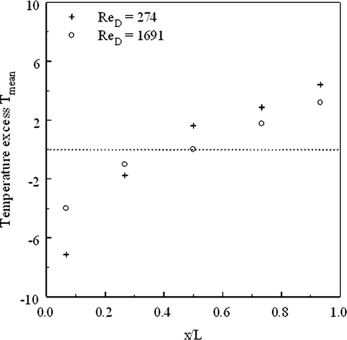
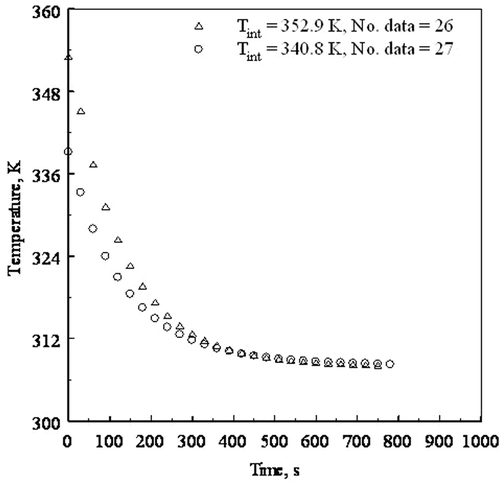
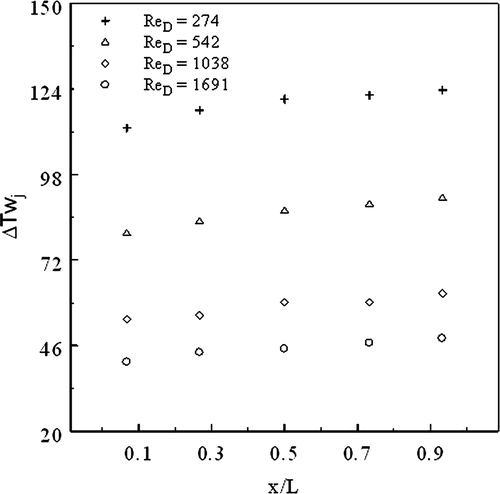
Though the heated plate is made intentionally as a lumped heat capacity system, it is noticed that the plate temperature is not uniform throughout. This is because the temperature distribution in the heated plate/wall is influenced by the porous medium that is in contact with the heated plate. Figure 2 shows the measured local temperatures (above ambient) of the plate at steady state for different Reynolds numbers corresponding to a given maximum value of heat input 104.6 W. It is evident from the figure that the temperature distribution is more uniform at higher Reynolds number. Figure 3 presents the temperature excess from the mean value of plate temperature estimated at various dimensionless distances of the heated wall at low and high Reynolds number cases. As seen from this figure, the maximum deviation from the mean value of plate temperature is 7°C at Reynolds number, Re_D = 274 and at Reynolds number Re_D = 1691, the maximum deviation is only less than 4°C. This shows that for higher flow rates, the spatial temperature variation is only marginal and more importantly the temperature recorded by a thermocouple located at the non-dimensional distance, x/L = 0.5 is very close to the mean value of plate temperature. It is, therefore, inferred that when the local temperature variation is marginal, the thermocouple which records the temperature closest to the average plate temperature is the right choice to represent the gross behaviour of the system. In view of this, the isothermal assumption of the heated wall is considered to be valid only if the spatial variation of temperature with respect to the mean value is less than ±4°C. In fact, this conclusion is arrived at from the observation that when the initial local temperature variation of the heated wall is less than ±4°C, with respect to the mean value of plate temperature, the values of the parameters (i.e. a, b and c) in the Nusselt number correlation retrieved through solving the inverse problem agree consistently. Moreover, the interferometer studies performed in our laboratory 18 on the heated aluminium plate under natural convection show that the local Nusselt number agrees well with the Ostrach 19 solution which is an accepted benchmark solution for a vertical isothermal flat plate. The foregoing analysis reveals that if the local temperature variation along the length of the plate is marginal, the heated wall can be considered to be isothermal and in view of this the temperature recorded by a thermocouple that shows temperature close to the average plate temperature is used for the estimation of the average heat transfer rate from the plate during cooling. However, even though the heated plate is thermally lumped, the isothermal assumption of the heated wall becomes invalid at high heat flux values and under such conditions the parameter estimation using the transient experimental data of the plate, which is idealized as a lumped heat capacity model, often leads to unrealistic results. Hence, it is worth mentioning that among the transient experiments conducted, the temperature–time data of experiments for which the initial local temperature variation is less than 4°C, with respect to the mean of plate temperatures, are only considered for the parameter estimation using the transient experimental technique proposed here. The key point in the transient technique employed in this study is the assumption that the thermal equilibration of the plate, as it loses heat, is almost instantaneous. Such an assumption is truly valid for plate materials of high thermal conductivity that are at the same time not very thick. Characteristic transient temperature data of the plate while it cools from two different initial conditions are shown in Figure 4, together with the number of data points used in the inverse of analysis of each experiment.

Figure 2. Measured local temperature (above ambient) of the heated plate for different Reynolds numbers at a given power input = 104.62 W.

Figure 3. Temperature excess from the mean of plate temperature estimated at various dimensionless distances.

Figure 4. Measured transient temperature of the plate for two different initial conditions. (experiment numbers 4 and 1). Also shown is the number of temperature–time data of each experiment.

5. Results and discussion

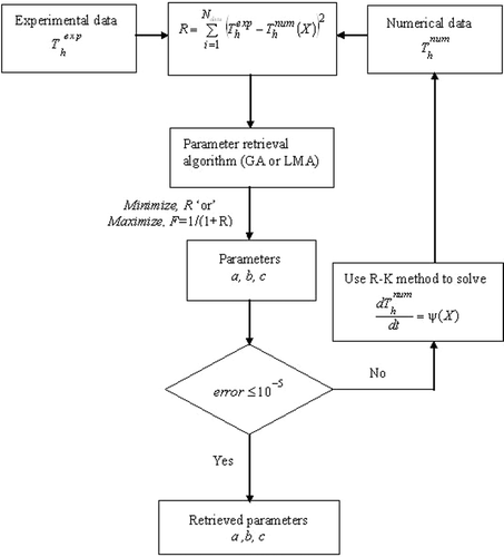
Figure 5 shows the route map for solving the parameter retrieval problem considered in this study. The search space used for the design variables, for the present problem is, . This provides maximum flexibility in probing global optima for each design variable. In fact, the bounds are a priori chosen for each design variable based on earlier studies conducted on channels filled with porous inserts reported in the literature. An in-house code is developed for LMA and the GA code originally developed by Carroll 20 is modified for solving the inverse heat transfer model. The programs are executed on a Pentium 4 machine with a 3 GHz processor and 2 GB RAM. Temperature data from nine transient cooling experiments, three for each porous sample (i.e. ϕ = 0.85, 0.89 and 0.92), with different initial temperatures were used for the parameter estimation. The temperature dependency of specific heat of wall material (aluminium) and the thermal conductivity of solid matrix (Cu alloy) are adequately addressed by a linear variation defined, respectively, as 21 and 9

Figure 5. Route map for solving the parameter retrieval problem.

Initially, the LMA is executed by assigning values of lower and upper bounds of the parameters as the initial guess. For a randomly chosen transient experimental data, when lower bounds of the parameters are used as the initial guess values for executing the LMA, the parameters are estimated as; a = 1.5, b = 0.1 and c = 0.47854. On the other hand, when upper bounds of the parameters are used as the initial guess values the solution yields, a = 0.70, b = 0.03 and c = 0.64385. When this exercise is repeated for another set of experimental data, the estimated parameters are, a = 1.5, b = 0.1, c = 0.46622, and a = 0.70, b = 0.03, c = 0.63555, respectively, when lower and upper bounds of the parameters are used for executing the program. Instead, when using GA, the initial population is randomly generated in the search space assigned for the design variables and even for a low number of generations (80) the algorithm predicts the values a = 1.07748, b = 0.03071, c = 0.55294, and a = 1.11877, b = 0.05928, c = 0.52682, respectively, for the respective experiments considered in LMA. It can be seen that the values of the parameters predicted by GA using the temperature time data of two transient cooling experiments are close to each other. Furthermore, the proximity of the values of retrieved parameters from all experimental trials indicates the global optimum of the parameters. This analysis once again establishes the observation made in previously reported studies that in probing global optima for multimodal problems using gradient-based methods with arbitrary chosen guess values from a large search space of the design variables, the solution may get trapped into a local extreme or even diverge. The foregoing analysis, therefore, establishes the need for hybridization of a stochastic method with a gradient-based optimization technique for the problem under consideration in order to blend the search ability of GA to locate the neighbourhood of the solution and, faster convergence and high level of accuracy in the estimated values at the optimum point provided by LMA.

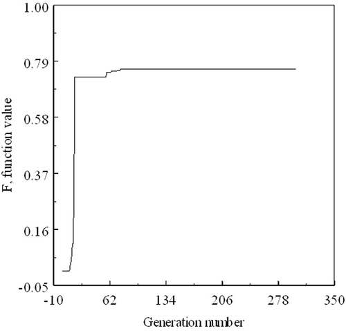
Table 1 indicates the values of parameters retrieved using GA from nine transient experiments, together with the time taken for carrying out a certain number of generations (iterations so to speak). As can be seen from the table, no appreciable change is observed between the values of parameters retrieved after 200 and 300 generations and therefore it can be inferred that after 200 generations, the estimated parameters have reached the optimum values. An inherent feature of GAs is that as they mimic mechanics of natural evolution; better and better values will be generated as the generations proceed. However, the improvement may often not be substantial from a mathematical viewpoint. In view of this, a subsequent implementation of a gradient-based method after some iterations with the GA may be appropriate for the refinement of the solution vector. It is clear from Figure 6 that the function value changes abruptly below 80 generations of GA which means the parameters are far away from their optimum values. No substantial change in the fitness function value ‘F’ after 150 generations is a clear indication of near-global optimum of the parameters. The convergence history curve also conveys a message to switch over to a gradient-based optimization algorithm immediately when GA locates a solution in the neighbourhood of the global optimum. Accordingly, with a view to reduce the computational time and to refine and improve the solution, the LMA is implemented with initial guess values taken from GA output after 80 generations. Table 2 shows the results of parameter estimation after 80 generations of GA, LMA implemented after 80 generations of GA and after 300 generations of GA, respectively, for each experiment. It is seen from the Table 2 (experiment number 1) that GA took 34.22 s to complete 80 generations, so as to arrive at a value close to optimum whereas LMA took just 1.81 s to converge the solution to the accurate values. A two-stage optimization that combines the complementary advantages of a stochastic and a gradient-based algorithm ensures accurate results with a reduction in computational time. This is more advantageous when a large number of parameters are to be estimated while handling more complex inverse problems. Figure 7 shows the estimated error between measured and simulated temperatures for a transient experiment (experiment number 5) when GA alone is used and GA combined with LMA are used. The proximity of experimental and simulated temperature is an indication that the parameter estimation is robust. A maximum error of 0.83 K that is observed during the initial phase of cooling process may be due to larger uncertainty in heat loss estimation induced by rapid cooling rate. The mean and standard deviation (SD) of the values of the retrieved parameters are estimated and are shown in Table 2. The rapid decrease in the value of the residual as the parameters ‘a’, ‘b’ and ‘c’ approach their optimum values is illustrated in Figure 8(a)–(c), respectively. The mean value of the parameters are then used to propose a Nusselt number correlation of the required form which is (18)

Figure 6. Convergence history of genetic algorithm.

Figure 7. Error between measured and simulated temperatures (corresponding to experiment number 5), GA* – output after 80 generations.

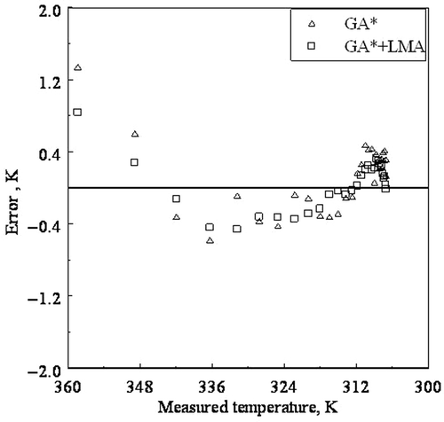
Figure 8. (a) Decrease of residual as the parameter, a approaches the optimum value; (b) Decrease of residual as the parameter, b approaches the optimum value; (c) Decrease of residual as the parameter, c approaches the optimum value.

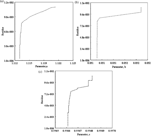
Table 1. Values of the parameters retrieved using GA.

			Retrieved parameters
Porosity	Initial temperature (K)	Number of generations	a	b	c	CPU time (s)
0.85	340.8	80	1.07749	0.03071	0.55294	34.22
		200	1.07748	0.03011	0.55312	65.97
		300	1.07774	0.03000	0.55312	105.55
0.85	350.9	80	1.08125	0.04403	0.56493	36.88
		200	1.08125	0.04406	0.56492	73.84
		300	1.08125	0.04406	0.56492	107.55
0.85	364.1	80	1.04410	0.05595	0.52522	37.20
		200	1.03753	0.05928	0.52500	75.39
		300	1.03750	0.05929	0.52500	125.23
0.89	352.9	80	1.11877	0.05928	0.526820	41.21
		200	1.05465	0.05999	.54609	82.17
		300	1.05465	0.05999	0.54610	126.22
0.89	358.8	80	1.06277	0.05998	0.54612	36.53
		200	1.06285	0.06000	0.54605	72.47
		300	1.06289	0.06000	0.54609	109.83
0.89	371.0	80	1.08785	0.05622	0.53556	44.08
		200	1.08758	0.05624	0.53556	88.11
		300	1.08796	0.05810	0.53454	133.59
0.92	387.7	80	1.06584	0.05997	0.55527	43.84
		200	1.21591	0.05988	0.53152	89.02
		300	1.25315	0.05998	0.52642	132.92
0.92	377.5	80	0.99581	0.05624	0.54738	37.05
		200	0.99375	0.05999	0.54494	71.54
		300	0.99376	0.05999	0.54492	107.51
0.92	369.8	80	1.10261	0.05988	0.53746	38.06
		200	1.11459	0.05999	0.53559	79.05
		300	1.11436	0.05999	0.53563	118.28

Table 2. Parameters retrieved using GA and hybridization of GA with LMA.

			Retrieved parameters
Porosity	Initial temp (K)	Algorithm	a	b	c	CPU time, s
0.85	340.8	GA*	1.07749	0.03071	0.55294	34.22
		GA* + LMA	1.01758	0.03524	0.54828	36.03
		GA**	1.07774	0.03000	0.55312	105.55
0.85	350.9	GA*	1.08125	0.04403	0.56493	36.88
		GA* + LMA	1.08161	0.04454	0.56417	38.82
		GA**	1.08125	0.04406	0.56492	107.55
0.85	364.1	GA*	1.04410	0.05595	0.52522	37.20
		GA* +LMA	1.03620	0.06042	0.52410	40.46
		GA**	1.03750	0.05929	0.52500	125.23
0.89	352.9	GA*	1.11877	0.05928	0.526820	41.21
		GA* + LMA	1.08436	0.05533	.54642	45.23
		GA**	1.05465	0.05999	0.54610	126.22
0.89	358.8	GA*	1.06277	0.05998	0.54612	36.53
		GA* + LMA	1.11346	0.06017	0.54486	41.76
		GA**	1.06289	0.06000	0.54609	109.83
0.89	371.0	GA*	1.08785	0.05622	0.53556	44.08
		GA* + LMA	1.09116	0.05741	0.53573	47.88
		GA**	1.08796	0.05810	0.53454	133.59
0.92	387.7	GA*	1.06584	0.05997	0.55527	43.84
		GA* + LMA	1.05986	0.05876	0.54971	47.90
		GA**	1.25315	0.05998	0.52642	132.92
0.92	377.5	GA*	0.99581	0.05624	0.54738	37.05
		GA* + LMA	1.05990	0.05744	0.55063	39.66
		GA**	0.99376	0.05999	0.54492	107.51
0.92	369.8	GA*	1.10261	0.05988	0.53746	38.06
		GA* + LMA	1.10882	0.05954	0.53934	40.92
		GA**	1.11436	0.05999	0.53563	118.28
Mean (GA* + LMA)	1.073	0.054	0.545
SD (GA* + LMA)	0.032	0.009	0.011
Notes: GA*, output after 80 generations; GA**, output after 300 generations.

Equation (18) is applicable for the range of non-dimensional parameters shown below.

The Peclet number exponent is close to 0.5, normally seen in laminar flows. The retrieved parameters have an SD of error, a = 1.073 ± 0.032, b = 0.054 ± 0.009 and c = 0.545 ± 0.011. A look at the range of non-dimensional parameters indicates that the proposed Nusselt number correlation is applicable for a narrow range of non-dimensional parameters and this is as opposed to a Nusselt number correlation developed using steady state experiments. This is because the temperature range encountered during a transient cooling experiment is limited, whereas an experimentalist generally has the freedom to choose wide range of temperatures in doing steady-state experiments. Additionally, at higher temperatures, the deviation from the isothermal nature of the plate and Boussinesq approximation becomes error prone and under such situations the mathematical formulation of the direct problem would not be adequate to represent physics of the problem. However, this approach has the advantageous feature that a large range of conditions can be covered in a single transient run, thereby giving a wealth of information from a large number of data points. This unique feature of the transient experiment demands that only a few transient experiments are required for estimating the unknown parameters in a heat transfer correlation.

5.1. Sensitivity study

A sensitivity study is carried out to test the robustness of parameter estimation supposing that measured temperature can be corrupted due to expected measurement errors that would occur randomly. This is done by imposing random measurement errors artificially to the measured temperatures defined as, , where is the corrected temperature, is the measured temperature, ‘σ’is the SD of the measurement error and ‘ω’ is a random number. Three cases with random noise level σ = 0.1, 0.2 and 0.3 were considered. The value of ω is randomly generated and chosen over the range −2.576 < ω < 2.576, which represents the 99% confidence bound for the temperature measurement. Table 3 shows the values of the parameters re-estimated after perturbing the measured temperatures with Gaussian noise for different values of σ. The values reported in Table 3 are the result of error analysis done for experiment 2. The results show that for small values of ‘σ’, the values of the retrieved parameters are consistent. However, for ‘σ’ = 0.3, the retrieved values of the parameters indicate that the measurement errors amplify the error in the estimated values. Moreover, the analysis indicates that the proposed method provides accurate and stable values of the parameters when a realistic error level is used. In general, from the results of the sensitivity study, it can be concluded that an increase in the measurement errors causes a decrease in the accuracy of the inverse solution, as expected.

Table 3. Values of the retrieved parameters using GA + LMA for different SD values of the measurement errors (i.e. σ = 0.0, 0.1, 0.2 and 0.3).

			Retrieved parameters
Case no	Initial temperature (K)	SD (σ)	a	b	c
2	350.9	0.0	1.08161	0.04454	0.56417
		0.1	1.03076	0.04359	0.57231
		0.2	1.08114	0.03002	0.56895
		0.3	1.17789	0.04765	0.54928

5.2. Comparison of inverse solution with direct result

The authenticity of the proposed correlation is tested by comparing the Nusselt number values predicted by the correlation with Nusselt number estimated directly from steady-state experiments. The average Nusselt number is estimated using the measured power dissipation at the wall and average wall temperature with respect to the fluid inlet temperature. The average Nusselt number is then estimated as (19) where the average wall temperature excess, with respect to fluid-free stream temperature is defined as (20)

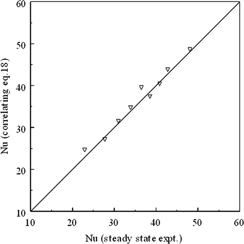
A comparison of the Nusselt number values estimated using the proposed correlation (Equation 18) and those evaluated from steady-state data is shown in the form of a parity plot in Figure 9. The comparison shows that the predicted values of Nusselt number using the correlation agree well with steady-state results. The validation exercise confirms the authenticity of the proposed approach for developing a heat transfer correlation by inverse method that consists of utilizing the transient data of a near isothermal plate integrated with numerical optimization procedures.

Figure 9. Comparison of Nusselt number estimated using the correlation, Equation (17) with steady state results.

6. Uncertainty analysis for steady experiments

The uncertainty_, ‘σ_Q’ in the dependent variable ‘Q’ is estimated according to the procedure outlined in [22], and this is given by (21) where ‘x’ stands for the independent variable and σ_x is the uncertainty associated with ‘x’. Following this procedure, the uncertainty in the estimation of heat flux is 2%, hydraulic diameter is 0.19%, effective thermal conductivity is 0.5%, average wall temperature with respect to fluid inlet temperature is 0.64% and the resulting uncertainty in the convective Nusselt number is estimated as 3.65%.

7. Conclusions

An inverse procedure based on transient heat transfer experiments combined with numerical optimization procedures is explored to develop a heat transfer correlation. The present approach works well on a system, having low thermal inertia for which quasi-thermal equilibration is almost established. A transient mixed convection experiment imparts a wealth of information by covering a wide range of conditions; therefore, only a fewer number of transient experiments are required for estimating the unknown parameters in the heat transfer correlation. The hybridization of a stochastic optimization method with a gradient-based method guarantees quick convergence to the optimum values of the parameters. A good agreement of Nusselt number values of steady-state experimental results with those estimated using the proposed correlation from the transient experimental technique reinforces the efficacy of the present approach. A Nusselt number correlation developed using transient experiments is applicable to a small range of non-dimensional parameters when compared to a Nusselt number correlation developed using steady-state experiments.

References

- Megerlin, FE, Murphy, RW, and Bergles, AE, 1974. Augmentation of heat transfer in tubes by use of mesh and brush inserts, ASME J. Heat Transfer 96 (1974), pp. 145–151.
- Renken, KJ, and Poulikakos, D, 1988. Experiment and analysis of forced convective heat transport in a packed bed of spheres, Int. J. Heat and Mass Transfer 31 (1988), pp. 1399–1408.
- Calmidi, VV, and Mahajan, RL, 2000. Forced convection in high porosity metal foams, ASME J. Heat Transfer 122 (2000), pp. 557–565.
- Pavel, BI, and Mohamad, AA, 2004. Experimental investigation of the potential of metallic porous inserts in enhancing forced convective heat transfer, ASME J. Heat Transfer 126 (2004), pp. 540–545.
- Raju, SK, and Narasimhan, A, 2007. Porous medium inter connector effects on the thermo hydraulics of near compact heat exchangers treated as porous media, ASME J. Heat Transfer 129 (2007), pp. 273–281.
- Pu, WL, Cheng, P, and Zhao, TS, 1999. An experimental study of mixed convection heat transfer in vertical packed channels, J. Thermophys. Heat Transfer 13 (1999), pp. 517–521.
- Reda, DC, 1988. Mixed convection in a liquid saturated porous medium, ASME J. Heat Transfer 110 (1988), pp. 147–154.
- Choi, CY, and Kulacki, FA, 1992. Mixed convection through vertical porous annuli locally heated from the inner cylinder, ASME J. Heat Transfer 114 (1992), pp. 143–151.
- Robinson, P, 1990. "Properties and Selection of Non Ferrous Alloys and Special Purpose Materials". In: ASM Metals Handbook, .. Vol. 2. Ohio, USA: ASM International Hand Book Committee; 1990. pp. 265–345.
- Nield, DA, 1991. Estimation of the stagnant thermal conductivity of saturated porous media, Int. J. Heat Mass Transfer 34 (1991), pp. 1575–1576.
- Massa, A, Franceschini, D, Franceschini, G, Pastorino, M, Raffetto, M, and Donelli, M, 2005. Parallel GA based approach for microwave imaging applications, IEEE Trans. Antennas and Propagations 53 (2005), pp. 3118–3127.
- Holland, J, 1975. Adaptation in Natural and Artificial Systems. Cambridge, MA: MIT Press; 1975.
- Goldberg, DE, 1989. Genetic Algorithms in Search, Optimization and Machine Learning. New York: Addison-Wesley; 1989.
- Deiveegan, M, Balaji, C, and Venkateshan, SP, 2006. Comparison of various methods for simultaneous retrieval of surface emissivities and gas properties in gray participating media, ASME J. Heat Transfer 128 (2006), pp. 829–837.
- Swaminathan, V, Gairola, RM, Balaji, C, Agarwal, VK, and Venkateshan, SP, 2008. Inverse radiation problem to retrieve hydrometeors from satellite microwave radiances, Int. J. Heat Mass Transfer 51 (2008), pp. 1933–1945.
- Marquardt, DW, 1963. An algorithm for least-squares estimation of nonlinear parameters, J. Soc. Indust. Appl. Math 11 (1963), pp. 431–441.
- Ozisik, MN, and Orlande, RB, 2000. Inverse Heat Transfer: Fundamentals and Applications. New York: Taylor & Francis; 2000.
- Krishna Sabareesh, R, Prasanna, S, and Venkateshan, SP, 2010. Investigations on multi-mode heat transfer from a heated vertical plate, ASME J. Heat Transfer 132 (2010), pp. 032501–032508.
- Ostrach, S, 1952. An analysis of laminar free convection flow and heat transfer about a flat plate parallel to the direction of the generating body force. NACA-TN-2635: Tech. rep.; 1952, Lewis Flight Propulsion Laboratory, NACA.
- Carroll, DL, 1996. "Genetic Algorithms and optimizing chemical oxygen-iodine lasers, developments". In: Wilson, HB, Batra, RC, Bert, CW, Davis, AM, Schapery, RA, Stewart, DS, and Swinson, FF, eds. Theoretical and Applied Mechanics. Vol. 18. F.F. Swinson School of Engineering, The University of Alabama; 1996. pp. 411–442.
- Venugopal, G, Deiveegan, M, Balaji, C, and Venkateshan, SP, 2008. Simultaneous retrieval of total hemispherical emissivity and specific heat from transient multimode heat transfer experiments, ASME J. Heat Transfer 130 (2008), pp. 061601-1–061601-8.
- Venkateshan, SP, 2008. About Measurement and Errors in Measurement – Mechanical Measurements. New Delhi: Ane Books India; 2008. pp. 5–25.