A semi-coupled solution algorithm in aerodynamic inverse shape design

Abstract

The numerical solution of an inverse airfoil design problem requires computational tools for grid generation, flow solution and the geometry update to provide the desirable shape corresponding to a given surface target pressure. Un-coupled as well as fully and semi-coupled shape design strategies have already been developed and employed. The target pressure is directly imposed in the fully coupled approach in contrast to un-coupled methods. Available semi-coupled methods use additional computational tools to couple the flow solver and the shape updater to directly impose the target pressure. In this article, a semi-coupled numerical shape design strategy is introduced, in the context of an ideal flow model, in which the target tangential velocity is directly imposed while no additional computational tool is employed. Numerical test cases, implemented on both structured and unstructured grids, are carried out to compare the performance of the proposed method with an adjoint-based optimization technique. Results show that the semi-coupled method has a two to three times faster convergence rate as compared to the adjoint approach. However, the semi-coupled solution convergence rate usually stalls after three orders of magnitude reduction of the objective function, while the un-coupled optimization method provides a more accurate solution. Therefore, a hybrid solution methodology is also advised, which provides faster convergence as well as lower computational errors as compared to both semi and un-coupled methods.

Keywords:

• aerodynamic inverse shape design
• direct design method
• adjoint-based optimization
• coupling strategies

1. Introduction

A thermo-fluid engineering problem in a prescribed shape of physical domain is described by governing equations, initial and boundary conditions and the relevant properties of the fluid. When all of this information is given and the objective is to find the field variables, such as pressure and velocity, the problem is referred to an analysis problem. When any of this information is unknown and the objective is to find the field variables as well as the missing information, the problem is referred to as an inverse problem 1.

Additional constraints are needed to render an inverse problem as a mathematically well-posed model. In an inverse shape design problem, the shape of part of the boundary of the domain is unknown and target values for some field variables are prescribed instead. For example, airfoils can be designed to achieve a prescribed surface pressure distribution in an aerodynamic inverse shape design problem 2,3 or ducts can be designed to prevent pressure over-shoot and under-shoot and to minimize the head loss due to the flow separation in viscous flows 4,5.

It is important to note that the aerodynamic inverse shape design problem is not well-posed in general and both the target pressure and the flow slip condition cannot be simultaneously satisfied on a given geometry. Shape design algorithms provide a means to find an appropriate geometry and to overcome the difficulties associated with the above-mentioned ill-posedness of inverse shape design problems.

A mathematical model associated with an inverse shape design problem can rarely be solved via analytical methods. Numerical techniques, on the other hand, are nearly always applicable. These numerical techniques are in general iterative due to the non-linearity of the flow model or the nature of the design algorithm. There are now powerful numerical schemes and simulation tools available that can be used to solve an aerodynamic inverse shape design problem via iterative procedures.

At least, three distinct computational tools are needed to develop a numerical algorithm for the solution of an aerodynamic inverse shape design problem. First, a grid generator/updater is needed to discretize the solution domain. Second, a flow solver/updater is needed to compute the flow variables at the nodal points and third, a shape generator/updater needs to be employed to change the existing shape to another one closer to the desirable geometry.

Numerical solution strategies in aerodynamic inverse shape design can be categorized based on the sequence of steps which are carried out to employ the above-mentioned computational tools. In an un-coupled solution strategy, the iterative design algorithm includes sequential calls to the grid generator, the flow solver and the shape updater. On the other hand, all three computational tools are employed simultaneously in a fully coupled design procedure. In semi-coupled numerical shape design methods, partial coupling strategies are used in the design iterations. It is worthwhile to mention that the shape optimization methods fall in the category of un-coupled shape design methods and the inverse methods correspond to the fully coupled methods.

Un-coupled solution methods date back to the primitive try and error solutions which are also the oldest and most widely used aerodynamic shape design methods. To respond to the need for the lower cost and faster design turn around, automated iterative design procedures, i.e. optimization techniques, have been developed. Advances in grid generation, computational fluid dynamics (CFD) and numerical optimization have been employed in sophisticated shape optimization algorithms. Examples of traditional gradient-based optimization methods can be found in 6–10. Evolutionary design algorithms, which are gradient-free global optimization techniques, have also been used in aerodynamic inverse shape design 11–14.

In an attempt to reduce the cost of the computation of the gradient of the objective function, which is the most expensive part of a gradient-based optimization loop, adjoint-based methods have been developed 15–17. Adjoint equation-based optimization methods are considerably faster than classical optimization techniques and are the preferred approach when the number of design variables is high. However, reduction of the computational cost comes with more mathematical complexity in the derivation of adjoint equations. The computational cost as well as the mathematical complexity of an adjoint-based optimization algorithm depends on the flow model.

In spite of the great achievements, the computational cost and complexity are still the major concerns in all un-coupled methods. The difficulties associated with the un-coupled inverse shape design methods are ultimately related to the fact that the target pressure is not directly imposed in such inherently iterative solution techniques. It is the search in a design space with an unknown topology that results in many shape corrections and the associated high computational cost.

Fully coupled solution strategies, in which the target pressure is directly imposed, have been developed as early as 1952 as reported in 18. However, in contrast to the un-coupled solution strategies, which are applicable with all flow models and two- or three-dimensional problems, early fully coupled methods could only be used in the context of simple flow models. For example, in the well-known Stanitzs’ method 18 the shape design problem is formulated using stream function and scalar potential as independent variables and, therefore, Stanitzs’ method is limited to the inviscid irrotational flow model. Borges 19 proposes a fully coupled shape design method limited to ideal flow fields as well. Borges’ method seems to be easier than Stanitzs’ method from the implementation point of view; however, there are convergence difficulties associated with the highly non-linear boundary conditions in Borges’ method. Ashrafizadeh et al. 2,5,20 developed a fully coupled shape design method which employs primitive flow variables and can be used, in principle, with all flow models in two- and three-dimensional solution domains. This fully coupled shape design method was called the direct design method. Taeibi-Rahni et al. 21 have employed the direct design approach to design ducts in the context of the Euler flow model. The direct design approach has not been applied in viscous flow shape design problems yet. However, successful implementation of the direct design of shape using the Navier–Stokes equations seems promising since the underlying concepts of the direct design approach were originally developed by Xu et al. 22 in the context of free surface viscous turbulent flows. Xu et al. 22 have shown that by imposing the calculated pressure on the surface of an oscillating body of water, the shape of the free surface can be recovered. The development of a viscous direct shape design algorithm is an ongoing research topic at the present time.

Fully coupled methods have their own pros and cons. The ultimate goal in any fully coupled shape design method is to solve the design problem with a computational cost comparable to the cost of one flow solution. Iterations in fully coupled methods, if necessary, are only due to the non-linearity in the equations which has to be dealt with in most of the practical flow problems anyway. This is in contrast to un-coupled methods in which many flow solutions are inherently needed in the solution algorithm. Therefore, in spite of the fact that, in practice, one fully coupled design solution is more expensive than one flow solution, the total computational cost of a fully coupled approach is often considerably less than the solution cost in an un-coupled method. This, as already mentioned, is due to the fact that the target pressure is directly imposed in fully coupled methods and effectively drives the shape evolution. The method proposed by Ashrafizadeh et al. 2,5,20 has the remarkable feature that the target pressure is imposed in a natural way by enforcing a conservation constraint, often the mass conservation, at the boundary cells in the context of finite volume method. In other words, no additional computational tools are needed to update the shape. The down side is that the coefficient matrix in a fully coupled algebraic model of an inverse shape design problem may become ill-conditioned in some applications. In such cases, regularization, or other treatments 2, may be necessary to obtain a solution.

The fully coupled strategy, mentioned above, is not the only option for directly imposing the target pressure. Semi-coupled methods can also be devised to update the shape by directly imposing the pressure. Van Den Braembussche 23 employs singularities on the surface of the body to impose the pressure and, therefore, distort the flow field around the body. The superposition of the induced flow and the free stream, results in new stream lines including the streamline corresponding to the body surface. Demeulenaere and Van Den Braembussche 24 relax the slip condition and allow the unknown boundary to be permeable to impose the target pressure. The imposed target pressure is applied to adjust the boundary location and to annihilate the transpiration velocity in an iterative procedure. Both strategies employ additional computational tools to couple the flow solver and the shape updater such that the target pressure is directly imposed. In the moving streamline approach of Van Den Braembussche 23, an induced velocity calculator is used to provide the required information for the shape update. Likewise, in the permeable wall strategy of Demeulenaere and Van Den Braembussche 24, an inverse Euler solver and the mass balance on evolving boundary cells need to be employed to update the shape. The computational cost for these semi-coupled methods is considerably less than for the optimization methods and is comparable to the fully coupled methods.

In this article, a semi-coupled shape design method is introduced which directly imposes the target pressure and does not need any additional computational tool. Therefore, it may be considered as an extension to the fully coupled method of Ashrafizadeh et al. 2,5,20. The proposed method is used to solve an inverse airfoil design problem. For the sake of simplicity and clarity, and to focus on the algorithmic issues, the ideal flow model is used. Regarding the computational mesh, an unstructured grid generator is employed and re-meshing is used to update the grid. To provide an overview on the coupling strategies and to compare the proposed method with some other alternative methods, the shape update procedures in an un-coupled adjoint-based optimization method, as well as fully coupled and semi-coupled solution strategies, are discussed in the context of the ideal flow model. Using the ideal flow assumption, the pressure and velocity are related through Bernoulli's equation and target pressure and (tangential) velocity can be used interchangeably. It is shown that the proposed semi-coupled shape design algorithm is easy to implement and converges faster than an adjoint-based optimization method. It is also shown that the proposed method can be used in a hybrid algorithm to boost the convergence rate of an un-coupled solution method.

The computational tools, needed in inverse shape design algorithms, are discussed first and design examples are presented afterwards.

2. The grid generator

Figures 1 and 2 show two discrete solution domains around two similar airfoils. The grid in Figure 1 is structured with quadrilateral elements and the grid in Figure 2 is unstructured with triangular elements. Each computational grid consists of a finite element background mesh and the corresponding set of non-overlapping finite volumes. The control volume around an arbitrary node is obtained by joining the midpoints of edges originating from that node. Integration points are defined at the middles of control surfaces (panels) as shown in Figures 1 and 2. Figure 3 shows a quadrilateral as well as a triangular element and the local coordinates of corresponding nodal points. Using the element shape functions N_j, any scalar φ with the local coordinates (s, t) in the element can be related to the nodal values of φ as follows: (1)

Figure 1. Domain discretization using structured grid.

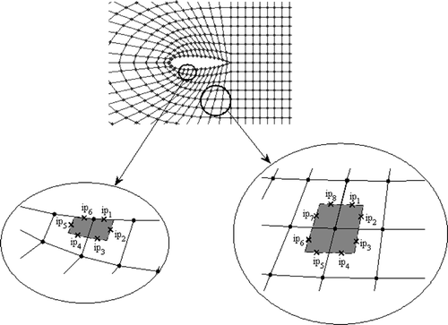
Figure 2. Domain discretization using unstructured grid.

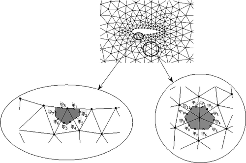
Figure 3. Local coordinates in (a) a quadrilateral element and (b) a triangular element.

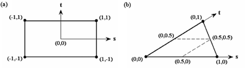
The summation index j takes values 1, 2 and 3 in a triangular element and 1, 2, 3 and 4 in a quadrilateral element. The grid generator provides the coordinates of nodal points as well as any mesh connectivity and other geometrical data required in the numerical solution. Here, the method of spines 2 is used to generate the required structured grids. Spines are basically coordinate lines provided by the user which render a two-dimensional grid generation problem into a one-dimensional grid generation problem. Regarding the unstructured grid, the standard Delaunay triangulation is used with a point insertion strategy borrowed from the advancing front method.

In a numerical inverse shape design procedure, the solution domain is not fixed and re-meshing or grid movement is necessary to comply with the evolving boundary. The grid updater takes care of this task during the shape evolution. In this study, re-meshing is used whenever a grid update is necessary.

3. The flow solver

The equations governing the fluid flow need to be discretized and solved on the discrete solution domain. Here an element-based finite volume method is employed to discretize an ideal flow field.

A two-dimensional ideal flow field can be completely described by the stream function governed by the Laplace equation. Satisfaction of the Laplace equation over a control volume corresponds to the balance of a flow-related variable F across the control surfaces as follows: (2)

It can be shown that 2: (3) and (4) where (5) and (6)

Einstein summation rule is applied to Equations (3)–(5). Points with the local coordinates (s₁, t₁) and (s₂, t₂) in Equation (6) are the end points of the control-volume surface panel containing the integration point ip 2.

A convenient form of F_ip can be developed for internal panels in analysis problems as follows: (7) where (8)

Note that G_m is a pure geometrical quantity. Therefore, the balance equation for an internal control volume can now be written as (9)

Equation (9) provides a constraint on the unknown ψ_p at an internal node.

At the boundary panels, another expression can also be used for F_ip to implement the boundary conditions: (10)

The balance equations for all boundary and internal control volumes are assembled to provide the following algebraic set of equations: (11)

A flow solution corresponds to the solution of the above linear set and provides the stream function values at all nodal points.

4. The un-coupled shape updater

An advanced gradient-based optimization method is discussed here as a representative of un-coupled shape design algorithms. Assuming that the airfoil shape is described by the design or control vector x, the update formula for the nodal coordinates on the airfoil body can be expressed as follows: (12)

In this equation, d is the search direction vector, scalar s is the step size and subscript k is the iteration number.

The design objective, or the cost functional, is defined as follows: (13)

Here, V and are the calculated and target tangential velocity values on the airfoil, respectively, and Γ_b is the surface area of the airfoil.

Starting with a user-specified initial guess for the design variables (x₀), methods are required to calculate the search direction and the step size to update the airfoil shape. The most expensive part of design iteration is the calculation of the search direction d_k which, in general, depends on the sensitivity of the objective function to each design variable. Therefore, the computational cost of one shape update in an un-coupled design solution is proportional to the computational cost of the calculation of the objective function gradient vector ().

The traditional gradient calculation method needs as many flow solutions as the number of design variables plus one. In fact, each design variable is perturbed and the corresponding value of the objective function is calculated. When this procedure is carried out for all design variables, the components of become available. By constraining each boundary node to move along the direction normal to the boundary at that point, there is only one design variable at each boundary node. Therefore, the number of design variables is equal to the number of boundary nodes.

The adjoint-based optimization method provides a clever approach to efficiently compute the required gradient. Instead of the objective function J, used in the original constrained optimization problem, the problem is converted to an unconstrained one and the Lagrangian L is minimized instead. Therefore, the components of the gradient of L are used to calculate the search direction. It can be shown that the ith component of the gradient of L is related to the flow solution ψ, the adjoint variable λ and the target velocity as follows 25: (14)

In Equation (14), V_i is the calculated tangential velocity, is the target tangential velocity, R_i is the local radius of curvature, λ_i is the nodal value of the adjoint variable, ψ_i is the nodal value of the stream function, and n_i is the normal outward direction at the ith nodal point on the airfoil. All the required information at the right-hand side of Equation (14) are obtained when the following two boundary value problems are solved 25. Equations (15) and (16) represent the flow and adjoint governing equations, respectively: (15) (16)

In Equations (15) and (16), Ω represents the solution domain and Γ_b and Γ_f stand for the airfoil boundary and the far field boundary, respectively.

Hence, considering the fact that the computational cost of the solution of an adjoint equation is roughly equal to the cost of a flow solution, the gradient vector in an adjoint-based design iteration becomes available at about the cost of two flow solutions. This is considerably less than the solution cost in classical optimization methods which require flow solutions as many as design variables in each iteration.

In gradient-based optimization methods, the gradient information is employed in the calculation of the search direction d_k. Numerical experiments have been carried out in the course of this study to choose appropriate methods for determining the search direction and also the step size. These experiments have shown that the steepest descent method with an experimentally determined piecewise constant step size function is very robust and converges fast as compared to higher order methods. Therefore, the steepest descent with piecewise constant step size are used in the solution of design examples in this article. With the search direction and step size available, Equation (12) is used to update the shape.

5. The fully coupled shape updater

In the fully coupled set of equations, which describe the shape design problem, both the nodal flow variables and the coordinates of nodal points need to be calculated. Therefore, the flow variable F_ip is linearized and re-written as follows: (17) which results in 2: (18)

Again, the balance equation for the control volume around the internal node P provides a constraint on ψ_p. Two additional required equations for x_p and y_p are obtained by grid generation equations, which can be written as follows 2: (19) (20)

The expression for the balance equation on control volumes around the airfoil is critically important in the fully coupled method. The target tangential velocity is imposed through the boundary control volume balances. A convenient form of the flow variable at a boundary panel, suitable for the conservative implementation of the target tangential velocity, is as follows: (21)

Note that the target pressure, or tangential velocity, is applied via the boundary control volume balance. The stream function value corresponding to the body of the airfoil is constrained by the Kutta condition 2. Two additional constraints are still needed at nodal boundary points. The boundary control volume balance, Equation (20), provides a constraint on one of the boundary nodal coordinates. The remaining coordinate at a boundary nodal point can be constrained through geometrical considerations. Here, each boundary node is constrained to move along the vertical direction (x_p = const) and the boundary control volume balance equation constrains the y-coordinate of the boundary node during the shape evolution. Hence, the number of constraints matches the number of unknowns for the nodal points along the airfoil.

Assembling all boundary and internal control volume balance equations results in the following fully coupled set: (22)

The vector u includes nodal unknowns ψ, x, and y. It is obvious that each solution of Equation (21) effectively corresponds to a simultaneous call to the grid generator, the flow solver and the fully coupled shape updater.

6. The semi-coupled shape updater

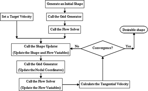
The fully coupled strategy just described requires the grid generation equations, which relate internal nodal coordinates to the boundary shape, to be built into the final algebraic set so that simultaneous upgrade of the shape and grid is possible. When node/cell generating algorithms are employed instead of grid generation equations, which is the case in classical unstructured grid generation methods, the shape and the grid cannot be computed simultaneously. However, it is still possible to solve the direct design equations on a background (lagged) grid. This strategy, therefore, separates the grid update from the update procedure for the flow and the shape and results in a two-stage prediction–correction procedure for each shape design iteration. In the prediction stage, the unknown coordinates of the internal nodes in the fully coupled shape design equations are replaced by the nodal coordinates of the existing grid. By solving the set of equations, the coordinates of the nodal boundary points are obtained. Therefore, the shape is updated in the prediction stage. The flow solution at this stage is a computational by-product that is discarded. With the new boundary available, the grid generator and the flow solver are then called in the correction stage to update the grid and the flow information, respectively. The semi-coupled shape design flow chart is shown in Figure 4.

Figure 4. The semi-coupled shape design algorithm.

7. A discussion on the coupling strategies

Now that a number of numerical shape design algorithms have been introduced, it is instructive to briefly review and compare the coupling strategies and to discuss a few important points.

In an un-coupled numerical shape design iteration, a grid generator, a flow solver and an un-coupled shape updater, e.g. an optimizer, are sequentially employed. This three-step design algorithm is inherently iterative.

In a fully coupled numerical shape design iteration, only a fully coupled shape updater needs to be called. Iterations in this one-step, or one-shot, algorithm are only required to resolve the non-linearities or to iteratively solve the set of linearized algebraic equations.

In a semi-coupled numerical shape design iteration, a fully coupled shape updater is employed followed by calls to the grid generator and to the flow solver. Iterations in this three-step design algorithm are inherently required to correct the errors due to the use of lagged grid information in the fully coupled shape updater. Therefore, the algorithm may be well-described as a two-stage prediction–correction algorithm as already explained.

While the semi-coupled strategy is often preferred when the unstructured grid generation is used, it has to be emphasized that all the above-mentioned coupling strategies are applicable with both structured and unstructured grid generators. For example, a semi-coupled strategy can be implemented in a code which uses a structured grid generator. Likewise, a fully coupled method can be used with an unstructured mesh which is updated by grid-governing equations. One scenario in the latter case is to model the initially generated unstructured grid with a net of linear springs. Consequently, the spring equilibrium equations are used for the unstructured grid update in a fully coupled manner.

The flexibility provided by the semi-coupled shape design strategy is important for the direct imposition of the target pressure in some aerodynamic inverse shape design problems. There are occasions in which the fully coupled shape design approach is not applicable. For example, numerical solution of shape design problems via mesh-less computational methods can be easily carried out using the semi-coupling methodology while, apparently, there is no way for fully coupled solution of such problems 26. Therefore, the semi-coupled numerical shape design approach may be the only, or the most convenient, algorithmic alternative for the direct imposition of the target pressure in some applications.

8. Results

8.1. Shape design example 1

The evolution of an initial circular shape to a symmetrical airfoil is considered here to examine and compare the un-coupled adjoint-based design method with the proposed semi-coupled approach.

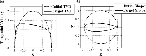
Figure 5 shows the target tangential velocity distribution corresponding to a symmetrical airfoil as well as the calculated tangential velocity distribution around the initial circular shape. Note that due to the symmetry, only half of the velocity diagrams are shown. Both the initial and final shapes are also shown in this figure. The boundary shape in this example is generated using 80 nodal points connected by straight line segments.

Figure 5. (a) The target tangential velocity distribution corresponding to a symmetrical airfoil and the tangential velocity distribution corresponding to the initial circular shape and (b) target airfoil as well as the initially guessed circular shape.

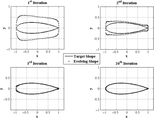
An adjoint-based optimizer using the structured grid shown in Figure 1 is used to update the shape starting from the circular section. A number of intermediate shapes during the design iterations are shown in Figure 6. The optimizer allows both x- and y-coordinates of boundary nodes to change during the iterations. Note that the shape is getting very close to the final shape after just three iterations.

Figure 6. The evolution of the shape during un-coupled design iterations.

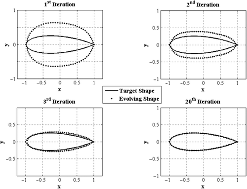
The proposed semi-coupled design method using the unstructured grid shown in Figure 2 is also used to update the shape starting from the same circular section. A number of intermediate shapes during the semi-coupled design iterations are shown in Figure 7. The x-coordinates of boundary nodes are fixed and the nodal points are only allowed to move in the y direction in this case. Again, the shape is getting very close to the final shape only after three iterations.

Figure 7. The evolution of the shape during semi-coupled design iterations.

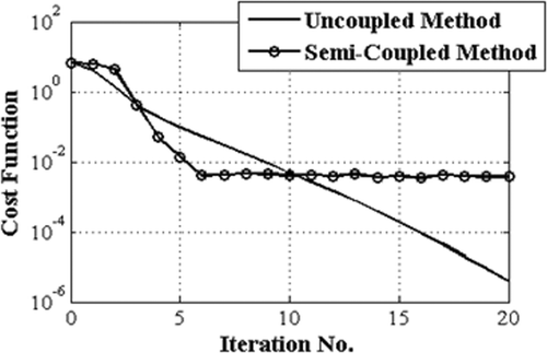
The convergence histories of the un-coupled and semi-coupled algorithms are shown in Figure 8. It is seen that the semi-coupled method converges faster initially but fails to make any further improvement after six iterations. The un-coupled method, on the other hand, provides a solution similar to the converged solution of the semi-coupled approach after 10 iterations, but continues to decrease the objective function and to obtain more accurate solutions after the 10th iteration.

Figure 8. Convergence histories of the un-coupled and semi-coupled design algorithms.

8.2. Shape design example 2

The evolution of a flat plate to an ellipse is considered as the second shape design example. Here again, 80 nodes are used to define the boundary geometry.

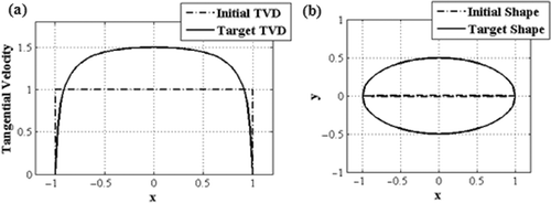
Figure 9 shows the target tangential velocity distribution corresponding to an ellipse and the uniform tangential velocity distribution along the flat plate. Once again, half of the velocity diagrams are shown due to the symmetry. Both the initial and final shapes are also shown in this figure.

Figure 9. (a) The target tangential velocity distribution corresponding to an ellipse and the tangential velocity distribution corresponding to the initial flat shape and (b) the target ellipse as well as the initially guessed flat shape.

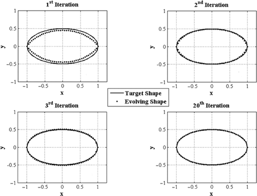
Figure 10 shows the convergence histories of the un-coupled and the semi-coupled algorithms. It is clear that the semi-coupled method has a higher initial convergence rate, but the un-coupled method provides a more accurate solution after a larger number of iterations. Therefore, to provide a better initial guess to the shape optimizer, a hybrid method is implemented in which a semi-coupled method is called first to rapidly improve the initially guessed shape. The performance of the hybrid algorithm is also shown in Figure 10, which clearly shows the convergence improvement of the un-coupled method. Figure 11 shows the evolution of the shape when the hybrid algorithm is used.

Figure 10. Convergence rates of the algorithms used in the design example 2.

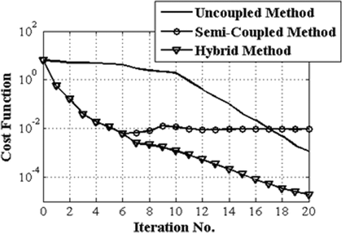
Figure 11. The evolution of the shape in the hybrid design algorithm.

8.3. Shape design example 3

The evolution of a flat plate to a cambered airfoil, using the proposed semi-coupled approach, is discussed here as the third shape design example. In this example, the boundary is described by 98 nodal points.

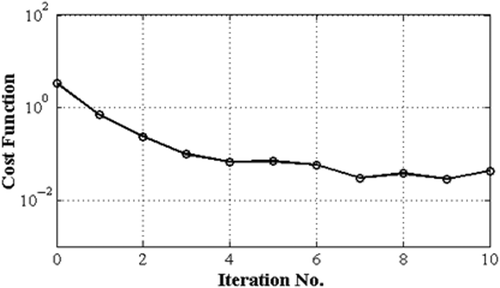
Figure 12(a) shows the tangential velocity distributions corresponding to the flat plate and the cambered airfoil shown in Figure 12(b). Note that in the case of the cambered airfoil, the flow field is not symmetrical and therefore the boundary velocity distributions are shown on both upper and lower surfaces. The evolution of the shape is shown in Figure 13. As we have already seen, the convergence rate of the semi-coupled method is initially very high and the initial guess gets close to the desired shape even after one design iteration. Figure 14 shows the convergence of the design iterations in this case. The semi-coupled solver reduces the cost function by nearly three orders of magnitude and stalls after seven iterations.

Figure 12. (a) The target tangential velocity distribution corresponding to a cambered airfoil and the tangential velocity distribution corresponding to the initial flat plate and (b) the target cambered airfoil as well as the initially guessed flat shape.

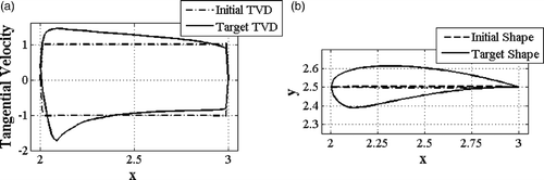
Figure 13. The evolution of the shape in the cambered airfoil design example.

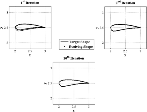
Figure 14. Convergence rate of the semi-coupled algorithm used in the design example 3.

9. A discussion on the computational results

The initial guesses in the design examples were chosen on purpose to be very far from the desired shapes in order to assess the robustness of the proposed semi-coupled method. It is clear that the method is robust in a sense that it does not fail regardless of the difference between the initial guess and the final geometry.

The proposed method, however, suffers from a relatively early convergence stall. In all of the above examples, the inverse solver stalls after nearly three orders of magnitude reduction of the cost function. In contrast, the un-coupled method, which calls for a direct flow solver, has a slower convergence rate but can provide more accurate solutions. These observations need to be rationalized. Here, we try to shed some light on the observed convergence behaviours of the coupled and un-coupled solution strategies and the associated computational expenses.

To compare the accuracy of the methods, we should note that the grids employed in the methods are not the same. Even though the un-coupled method employs a better grid near the boundary of the airfoil in our examples, and this may be partly responsible for the better convergence behaviour of the optimization method, however the grid quality cannot be blamed as the only culprit responsible for the early stall of the coupled design iterations. The authors’ previous experiences with the inverse shape design problems have shown that there are two characteristics associated with the convergence behaviour of fully coupled shape design methods. First, the rate of convergence of the iterations is initially very high and after a number of iterations becomes very low or zero (convergence stall). Second, the convergence level, or the magnitude of the cost function, is always higher than the level obtained in an un-coupled method used to solve a similar problem. The first characteristic seems to be common in all iterative algorithms, but the second observation needs further investigations. To the best of authors’ knowledge, the restriction on the convergence level of the coupled methods has something to do with the relatively high condition number of the coefficient matrices in these inverse formulations. The inverse shape design problem discussed in this article is not as ill-posed as some other inverse problems in science and engineering; however, the condition number of the coefficient matrix in the fully coupled shape design formulation is higher than the condition number of the coefficient matrix in the corresponding analysis problem, used in un-coupled formulations. In other words, the mathematical model of the inverse design problem, employed in the semi-coupled method, is not as well-posed as the mathematical model of the analysis problem employed in the un-coupled method. Therefore, the higher round off errors associated with the numerical computations in the coupled approach might explain the convergence stall at a higher value of the cost function.

Another observation regarding the convergence behaviour is that the driving force for the geometry modification in the semi-coupled method is directly related to the difference between the current boundary values of the tangential velocities and the target values. As the geometry gets closer and closer to the final shape, this driving force gets smaller and smaller and at some point is out-weighted by the numerical errors. This is the point at which the inverse solver stalls. This also happens in the un-coupled iterations; however, the numerical errors are less in this case as explained above. In any case, it is important to note that the solutions obtained by the coupled methods are practically acceptable in spite of the fact that the cost function of the shape design problem cannot be made as small as the machine zero.

The computational cost of one semi-coupled iteration, which includes a call to the inverse solver, the grid generator and the flow solver, is about the same as one un-coupled iteration, in which there is a call to the flow solver, the grid generator and the shape updater. This is due to the fact that the fully coupled (or inverse) solver has a computational cost close to the flow solver 2,5. It is important to note that this comparison is made only for the adjoint-based optimization techniques, for which the computational cost of each shape update is about the cost of a flow solution. If classical optimization techniques were employed, the computational cost of each un-coupled iteration would be much higher than a semi-coupled iteration.

Further studies are underway to better understand and to improve the convergence behaviour of the fully and semi-coupled shape design methods.

10. Conclusion

Three classes of algorithms for the solution of aerodynamic inverse shape design problems in the context of ideal flow model were discussed in this article. The classification was based on the sequence of steps required to update the shape in each design iteration. In an un-coupled method, a three-step procedure was carried out which included sequential calls to the computational tools, i.e. the grid generator, the flow solver and the shape updater. A fully coupled approach was also introduced in which all the computational tools were simultaneously employed in a one-shot algorithm. In the proposed semi-coupled algorithm, a two-stage, prediction–correction, procedure was carried out in each design iteration to improve an initially guessed shape far from the desired shape. It was shown that the proposed semi-coupled algorithm converges faster to an acceptable result and has a lower computational cost as compared to the un-coupled solution algorithm. Numerical shape design test cases were presented to show the applicability of the proposed semi-coupled algorithm as a stand alone shape design algorithm or as a booster to a shape optimizer. Based on the numerical experiments in this study, the semi-coupled approach seems to have to be two to three times faster than the un-coupled method to achieve a practically acceptable convergence level.

References

- G.S. Dulikravich, T.J. Martin, and B.H. Dennis, Multidisciplinary Inverse Problems, 3rd International Conference on Inverse Problems in Engineering, Port Ludlow, WA, USA, 1999..
- Ashrafizadeh, A, Raithby, GD, and Stubley, GD, 2004. Direct design of airfoil shape with prescribed surface pressure, Numer. Heat Transfer 46B (2004), pp. 505–527.
- Giles, MB, and Drela, M, 1987. Two-dimensional transonic aerodynamic design method, AIAA J. 25 (1987), pp. 1199–1206.
- A. Scascighni, A numerical method for the design of internal flow configurations based on the inverse Euler equations, Ph.D. thesis, Swiss Federal Institute of Technology, Zurich, 2001..
- Ashrafizadeh, A, Raithby, GD, and Stubley, GD, 2003. Direct design of ducts, J. Fluids Eng. 125 (2003), pp. 158–165.
- Hicks, RM, and Henne, PA, 1978. Wing design by numerical optimization, J. Aircraft 15 (1978), pp. 407–412.
- Rizk, MH, 1982. A new approach to optimization for aerodynamic application, J. Aircraft 20 (1982), pp. 94–96.
- Drela, M, 1988. Low-Reynolds-number airfoil design for M.I.T Daedalus prototype: A case study, J. Aircraft 25 (1988), pp. 724–732.
- Lee, KD, and Eyi, S, 1992. Aerodynamic design via optimization, J. Aircraft 29 (1992), pp. 1012–1019.
- P. Sturdza, An aerodynamic design method for supersonic natural laminar flow aircraft, Ph.D. diss., Department of Aeronautics and Astronautics, Stanford University, 2003..
- Failer, WE, and Schreck, SJ, 1996. Neural network: Applications and opportunities in aeronautics, Prog. Aerosp. Sci. 32 (1996), pp. 433–456.
- Fainekos, GE, and Giannakoglou, KC, 2003. Inverse design of airfoils based on a novel formulation of the ant colony optimization method, Inverse Probl. Sci. Eng. 11 (2003), pp. 21–38.
- Hacioglu, A, and Ozkol, E, 2003. Transonic airfoil design and optimisation by using vibrational genetic algorithm, Aircraft Eng. Aerosp. Technol. 75 (2003), pp. 350–357.
- Hacioglu, A, and Ozkol, E, 2005. Inverse airfoil design by using an accelerated genetic algorithm via distribution strategies, Inverse Probl. Sci. Eng. 13 (2005), pp. 563–579.
- A. Jameson and T.V. Jones, Optimum transonic wing design using control theory, Report for Air Force Office of Science Research under grant no. AFF49620-98-1-2002, 2002..
- Yiu, KFC, and Mak, KL, 2005. Airfoil design via optimal control theory, J. Ind. Manage. Optim. 1 (2005), pp. 133–148.
- Rajab, SA, 2004. Shape optimization of surface ships in potential flow using an adjoint formulation, AIAA J. 42 (2004), pp. 296–304.
- Stanitz, JD, 1988. A review of certain inverse methods for the design of ducts with 2 or 3-dimensional potential flow, Appl. Mech. Rev. 41 (1988), pp. 217–238.
- Borges, JE, 2007. Computational method for the design of ducts, Comput. Fluids 36 (2007), pp. 480–483.
- Ashrafizadeh, A, Raithby, GD, and Stubley, GD, 2002. Direct design of shape, Numer. Heat Transfer 41B (2002), pp. 501–520.
- Taeibi-Rahni, M, Ghadak, F, and Ashrafizadeh, A, 2008. A direct design approach using the Euler equation, Inverse Probl. Sci. Eng. 16 (2008), pp. 217–231.
- W.X. Xu, G.D. Raithby, and G.D. Stubley, Application of a Novel Algorithm for Moving Surface Flows, 4th Annual Conference of the Computational Fluid Dynamics, Society of Canada, 1996..
- A. Van Den Braembussche, The application of the singularity method to blade-to-blade calculations, in Thermodynamics and Fluid Mechanics of Turbomachinery, A.S. Ucer, P. Stow, and C. Hirsch, eds. (Nato Advanced Sciences Institutes Series, Series E, Applied Sciences, no. 97A), Martinus Nijhoff, Leiden, The Netherlands, 1985, pp. 167–191..
- Demeulenaere, A, and Van Den Braembussche, A, 1999. A new compressor and turbine blade design method based on three-dimensional Euler computations with moving boundaries, Inverse Probl. Sci. Eng. 7 (1999), pp. 235–266.
- O. Gecer, Shape optimization theory and applications in hydrodynamics, M.Sc. thesis, MIT, 2004..
- A. Ashrafizadeh, V. Esfahanian, and H. Bazmara, Direct Design of Shape Using a Meshless Computational Method, 21st Canadian Congress of Applied Mechanics, CANCAM 2007, Ryerson University, Toronto, Ontario, Canada, 2007..