Solution of inverse ODE using Bezier functions

Abstract

The identification of the actual form of the differential equation and the boundary conditions from a set of discrete data points has been a challenging problem for many decades. A unique two-step approach developed in this article can solve this particular inverse boundary value problem. In the first step, the data are fitted using the best Bezier function. Parametric Bezier functions, based on Bernstein polynomials, allow efficient approximation of smooth data and can generate the derivatives. Bezier functions are also good at handling measured data. The Bezier fit is smooth and large orders of the polynomials can be used for approximation without oscillation. In the second step, the known derivatives are introduced in a generic model of the differential equation. This generic form includes two types of unknowns, real numbers and integers. The real numbers are part of the coefficients of the various terms multiplying the derivatives, while the integers are exponents of the derivatives. The unknown exponents and coefficients are identified using an error formulation through discrete programming. This article looks at homogeneous ordinary differential equations (ODEs) and demonstrates it can recover the exact form of both linear and nonlinear differential equations. Two examples are solved. In both cases, the objective is to identify the exact form of the differential equation. The given data are exact, smooth and they represent solutions to known differential equations.

Keywords:

• inverse problem
• ordinary differential equations
• Bezier function
• data approximation
• MATLAB

1. Introduction

Inverse problems, particularly boundary value problems (BVPs), are an important area of research 1. Many problems in heat transfer, electromagnetism, medical imaging, seismology and remote sensing are solved as inverse problems 1–4. Reference 5 recognizes five kinds of inverse problems. The first kind is classified as shape determination inverse problem. It is about discovering the shape in the design domain. A popular application area is aerodynamic shape optimization. Reference 6 uses Bezier functions to obtain airfoil shape corresponding to prescribed aerodynamics coefficients. The second type of inverse problem establishes boundary conditions or initial values, particularly during experiments, at points that are not easily accessible. In many of these problems, there is usually excess information at other points on the boundary 2,7. The third kind of inverse problem establishes unknown field properties on the domain tied through the differential equations 8,9. The fourth kind of inverse problem determines material properties which are used in known form of the differential equations to match the solution 9–11. The last kind, the type addressed in this article, will determine the governing differential equation that yields the known solution to the problem 12,13. Most of the current work in this area is based on discretization methods like the finite element method and the boundary element method. The typical application domain is two dimensional with few papers in three-dimensional domain 14. There are several papers on one-dimensional problem 11,12. Additionally, there are some unique approaches to the inverse problems through probability 15 and neural nets 16.

The forward or the direct BVP is the determination of the solution everywhere if the differential equation is known and the boundary conditions are given. The natural inverse BVP will be to find the differential equation and information on the boundary if the solution is known on the domain. This is the fifth kind of problem mentioned earlier. In this article, the inverse problems determine a single homogeneous ordinary differential equation (ODE) from the data representing the solution. The procedure involves two steps. In the first step, the best Bezier function is fitted to the data. Parametric Bezier functions, based on Bernstein polynomials, allow efficient approximation of the data and the required derivatives for the entire range of the independent variable. The second step is to identify the specific form of the differential equation from a generic representation. This generic form is based on the expected form of the ODE.

Bezier functions can provide explicit solutions to several types of mathematical problems. Here, explicit solutions imply that the solution can be represented as a closed form polynomial with respect to a parameter. This is true even for problems where the known solutions are not polynomials. References 17–19 illustrate that Bezier functions, coupled to standard optimization, can be used to provide explicit solutions to many types of differential equations. These papers have shown that the same procedure can solve linear or nonlinear, single or coupled, ODE or partial differential equation (PDE), with initial and/or boundary values. Reference 20 is the application of Bezier functions to one- and two-dimensional data analysis. It illustrates that Bezier functions provided excellent approximations to smooth and non-smooth data, and that high order polynomials are quite well-behaved in expressing the data.

Bezier functions are parametric curves that are constrained to behave like a function. Bezier 21 defined these curves initially for automotive body definition as they were aesthetically engaging. These curves/functions are also constructed using the Bernstein or binomial basis functions. They are also a special class of the uniform B-splines using an open knot vector 22,23. The use of Bezier function in its parametric representation is an original approach pursued by the author. The matrix representation of these functions allows array processing that can improve the speed of computation.

Two examples are used to illustrate the method developed in this article. In the first example, the given data are generated using a linear differential equation, namely the Bessel equation. In the second example, the data are obtained from solving a nonlinear BVP, the Blasius equation. The solution for the latter problem represents the velocity distribution in the boundary layer. In both examples, the input data are smooth and completely represent the solution over the domain. Comparison is made through statistics and plots.

2. Bezier functions

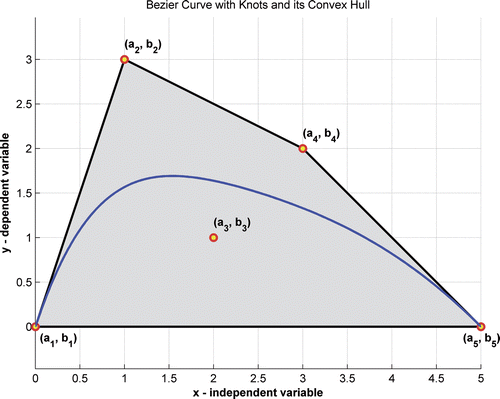
A Bezier function in two dimensions is a Bezier curve constrained to have the properties of function by requiring the independent variable x to monotonically increase as the parameter ranges from 0 to 1. In the parametric form of this Bezier function, instead of the explicit dependence of y with x, expressed as y(x), the pair of values (x, y) implicitly corresponds to the same value of the parameter p. The Bezier function described by the Bernstein or binomial basis can be expressed as 22 (1) (2) where represents the Bernstein basis and B_i's are the vertices or knots of the polygon (a pair of values a_i and b_i) that determine the function in two-dimensional space. Figure 1 illustrates the Bezier function. The polygon vertices are shown as circles and identified by a pair of values for a and b. The curve and all its derivatives can be obtained through simple arithmetic operations using these vertices. The order of the curve is n, one less than the number of vertices, which is the highest order of the polynomial in the basis. The Bezier curves are very smooth and can simulate all functions over an appropriate interval. Several properties of the Bezier functions make them very useful for approximating other functions.

Figure 1. Bezier curve/function definition.

Bezier functions can be defined through matrices. This makes computing the curves and derivatives easy. The curve in Equations (1) and (2) can be generated through the matrix multiplication of three terms 22 (3) where [P] is the parameter vector, a placeholder for parameter values between 0 and 1. [N] is the matrix of coefficients that depends only on the order of the curve, and [B] is the matrix of the vertices of the curve, [a b]. For the fourth-order function in Figure 1, the various matrices are:

2.1. Data decoupling

Equation (3), for two-dimensional Bezier function, can be recognized as leading to the decoupling of x and y data (4)

2.2. Data fitting with Bezier functions

The Bezier function corresponding to a given set of data points can be identified through the sum of the least-squared error (LSE) between the original data and the approximation. The application of this measure to either vector or array data yields a non-iterative algebraic relation that establishes the vertices of the Bezier function.

The LSE problem is framed as: given a set of n data points y_a,i, (or vector Y), and the order for the Bezier function m, find the coefficient vector, [B_y] so that the squared error generated by the approximate data y_b,i, (or vector Y_B) is the smallest. (5) where P_A is the complete parameter matrix for all of the points. [B_y] is found using standard calculus as (6)

Equation (6) establishes the best coefficient matrix [B_y] for a given order of the Bezier function. This non-iterative approach allows us to add additional processing to choose the best order for a given set of data. In this article, the best order is based on the sum of the absolute error over all of the data points. This sum initially decreases with increasing order and then starts to increase after a certain order has reached. The minimum value of the sum of the absolute error provides the best order for the Bezier function. It is implemented as follows:

1.	Choose a starting order for the Bezier function that will fit the data.
2.	Find the Bezier coefficients using LSE or through (6)
3.	Find the sum of the absolute error.
4.	Increment the order by one and calculate the change in the absolute error.
5.	If the absolute error decreases, then the order is increased by one, and the processing is returned to Step 2. If it increases, then this current order and coefficients will determine the best Bezier function.

The following section illustrates the effectiveness of the Bezier function in approximating the data and the derivatives.

2.3. Data with derivative singularity

The procedure proposed in this article relies on the effective approximation of the data and its derivative content through Bezier functions, particularly for non-polynomial functions. In the first example, the original data lie on the quarter circle (7). There are 31 data points. The maximum best order permitted was 10. Figure 2(a) illustrates that the Bezier function approximates the original data very well. The average absolute error of the approximation was 2.073e–012. (7)

Figure 2. (a) Original data and Bezier representation for quarter circle. (b) Original and Bezier derivatives for quarter circle.

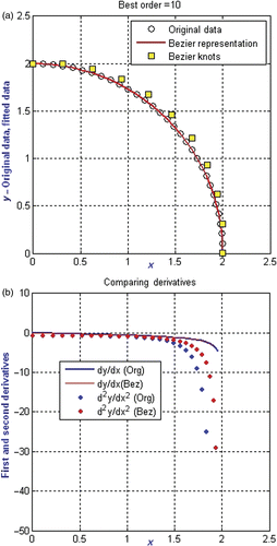
Figure 2(b) is the comparison of the derivatives based on (7) and those based on the Bezier function. The first derivative is singular at (2, 0). The solid lines compare the first derivatives and they match up very well till the point of singularity. The second derivatives match well until x = 1.5, after which it is overestimated by the Bezier function. In this example, the data points are not equidistant.

2.4. Non-polynomial data

The typical solution to linear BVP involves exponential and trigonometric functions. We use the relation in (8) to create the data points. (8)

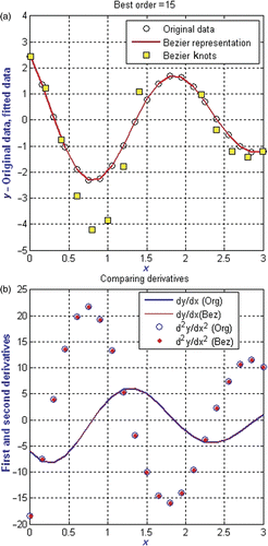
Figure 3(a) is the comparison of the original data and Bezier approximation. The average absolute error over 21 equidistant points is 9.554e−009 ensuring that the quality of the approximation is excellent. The maximum order of the Bezier fit is 15 which correspond to about five orders for each change in the curvature. Figure 3(b) is also impressive. The first and second derivatives generated by the original function in (8) and those by the Bezier approximation are very close. In fact, within the scale of the figure, there appears to be no change in the first derivatives. Both these examples suggest that data and derivative approximation by Bezier functions are justified. For data which are very difficult to approximate, the method proposed by this article will not be useful.

Figure 3. (a) Original data and Bezier representation for Equation (8). (b) Original and Bezier derivatives for Equation (8).

2.5. Measured data

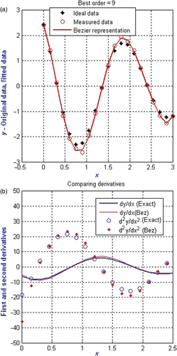
The examples illustrated in previous sections were based on smooth data. For inverse problems, the available data are usually not smooth. A stochastic interpretation of the data is often performed. In this section, we illustrate that the Bezier function can capture the essential information in the data without additional processing. The best Bezier approximation will smooth the data around the data mean. We generate the measured data using the MATLAB rand function as expressed in (9). (9)

Figure 4(a) illustrates the original smooth data, the perturbed data and the Bezier approximation over 21 points. The average absolute error is 2.797e–002. The Bezier approximation appears to pass through most of the perturbed data. Figure 4(b) compares the derivatives of the Bezier approximation with the derivatives of the original smooth data. It can be seen the derivatives are estimated reasonably well even though the Bezier approximation deals with the perturbed data.

Figure 4. (a) Measured data and Bezier function. (b) Comparison of Bezier derivatives.

2.6. Data extrapolation

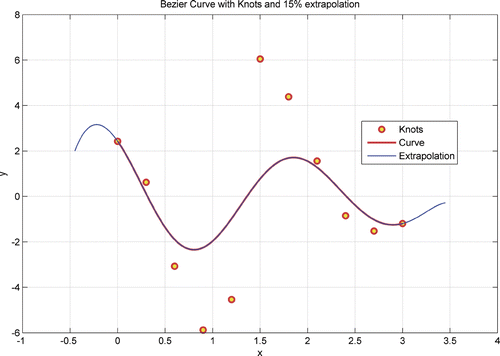
In inverse problems, sometimes the data are available only in a part of the domain. It may be necessary to extend the behaviour by extrapolation. Figure 5 illustrates a 15% extrapolation on either side of the data that was used for the approximation. The range of the original data is indicated by the Bezier knots (or vertices). By definition, the first and the last data points coincide with the end vertices. You can see that the extrapolation captures the content of the original data, including a peak in the left end. Technically, the extrapolation is not a Bezier function by definition, as the parameter is not restricted between 0 and 1.

Figure 5. Extrapolation using Bezier approximation.

2.7. How many data points?

Additional examples can be created to support the contention that the Bezier function approximation is excellent in representing the original data and developing information on its derivative content, essential knowledge for identifying the actual form of the BVP.

An important question for this procedure is the maximum permissible order of the Bezier function. Numerical experiments by the author suggest that for smooth data, the maximum order of 15 be used to avoid round off error in 32-bit architecture machines using double precision. This means the data should have no more than three changes in curvature. For non-smooth data it is recommended to reduce the order below 10 to make derivative computation more stable. The Bezier approximation tries to capture the oscillation of the mean about the data.

The second question is the number of original data points needed for the procedure. For smooth data, this is not a problem as the number of data points can be the same as the number of Bezier vertices. For non-smooth data, the author recommends at least double that of the order of the Bezier function.

One important information not exploited in this study is that the mean of the original data and the best Bezier approximation is very close for both smooth and perturbed data.

3. Solution to the inverse problem

The solution to the inverse problem in this article is to identify the actual form of the differential equation and the boundary conditions, which when integrated should yield the original discrete x, y data. The original data represent the function itself whose form is not known. We split the solution process into two distinct steps.

In the first step, the discrete data are fitted with the best Bezier function according to Section 2.2. We will call it f(x), knowing that it will be handled through the parameter representation [x(p), f (p)] primarily through a set of vertices. The given data are now connected with a function. In addition, a sufficient number of its derivatives can also be evaluated over the range of the function. The function value and the derivatives at the initial and final boundaries provide the necessary boundary conditions for the BVP. The original data and the data fitted using a Bezier function can also be compared using standard data statistics. A good fit in the statistics indicate that the original data can be represented by the corresponding Bezier function.

In the second step, a generic form of the differential equation is chosen. The values for the derivatives to be used in this generic form are obtained from the knowledge of the vertices and are completely known from Step 1. Reference 23 is certain that the Bezier function is excellent at capturing derivative content in the data. If the generic form is broad enough to include most of the popular forms of the differential equation, then this study should have merit. This generic form will contain many coefficients and integers, which once solved, will establish the specific form of the differential equations whose solution is the original data.

Choosing a particular generic form for the differential equation restricts the solution to differential equations of a particular class. Several generic forms of third order, homogeneous, ODE are given below. These generic forms are based on the particular examples investigated in this article. Similar forms for fourth order or second order can be established. A constant coefficient linear ODE will be represented by (10)

A generic form for constant coefficient nonlinear ODE will be (11)

A variable coefficient linear ODE can be represented by (12)

A variable coefficient nonlinear ODE will be represented by (13)

In all the generic forms, there are two types of unknowns: the exponents of the derivatives and the coefficients in the terms multiplying the derivatives. The exponents are expected to be integers. The coefficients multiplying the terms are unrestricted. The function and its derivatives in the generic form are known after Step 1.

3.1. Establishing the unknowns

Several points (N) in the range of the independent variable are used to evaluate the residuals of the generic form. These can be independent of the number of original data points as they are derived from the Bezier approximation. These residuals are then used to set up the LSE problem. For example, using the generic form in (11) we can express the objective function as (14)

All the unknowns are expected to be real. Using a traditional real unconstrained optimizer exposed two problems. First, the exponent values were not integers in spite of tight side constraints on them. This can be overcome by considering the exponent unknowns to be integers and shifting to a mixed integer and real programming problem. This approach did not yield satisfactory results as the optimized solution did not vary much from the initial guess. The second problem was more serious because the numerical techniques kept determining the trivial solution. (15)

A useful solution must avoid this trivial result which will impact the search for the optimum solution.

3.2. Establishing the unknowns – discrete programming

The fact that the exponents are integers with only limited possible values suggests that one can easily cycle through this limited set of integers and arrive at a solution. If the coefficients are real numbers, then continuous value for the coefficients cannot avoid the trivial solution. Even if the trivial solution is penalized, the solution will be closest to the non-penalized value for the coefficients. This implies that the solution is already predetermined. To find a useful solution, we will have to make another assertion. Each coefficient will belong to a set discrete numbers. This changes the problem into a discrete optimization problem. Discouragement of the trivial solution will have to be a part of the technique.

3.3. Solving the discrete programming problem

There are only limited techniques for solving the discrete optimization problem 24. The best solution, being a trivial one, further restricts the techniques. The easiest of the discrete methods is exhaustive enumeration where all the values for the unknowns are considered in combination before the optimum is determined. For the form in (14), allowing three values for the exponents and three values for the discrete coefficients, the amount of time required for computation was around a staggering 1.0 × 10⁵ CPU seconds. This was based on a Linux machine running MATLAB and the simple code comprised only a set of nested loops.

The second approach is to run the discrete optimization problem using heuristic programming. In this article, a simple heuristic exhaustive enumeration over predetermined number of cycles was implemented. About 1 billion cycles were identified to be reasonable from using exhaustive enumeration. This will only work for a limited choice of discrete variables.

A third approach is to use global search techniques. This permits a larger set of discrete choices for the coefficients. The genetic algorithm (GA) from the MATLAB toolbox is used to solve Example 2 in this article.

3.4. Computational resource

The software used to implement the examples and create the plots is MATLAB®. The computation involving enumeration was mostly performed on a symmetric multi-processor (SMP) machine with two dual core AMD Opteron processors rated at 2.8 GHz, 32 GB of main memory. Many different strategies were explored to keep the time of computation small. The primary one was to limit the discrete data set for the variables. The computations involved are quite simple and can be programmed in any software and executed on any platform.

4. Examples

There are two examples in this section. Both of them are based smooth data. Examples with perturbed data are under investigation. It is possible to obtain a solution with the perturbed data; however, there are some fundamental issues that are not yet clear to the author. One of them is the justification for expecting the differential equation identified by the perturbed data to match the differential equation identified by the smooth data which generated the perturbed data. The boundary conditions are no longer the same for both problems. Results so far do not support this hypothesis. The first example involves the identification of the linear ODE based on a set of smooth x–y data. The second example discovers the form of a nonlinear ODE from a set of smooth x–y data. Initially, specific generic forms were used to control the time of computation. The more liberal generic form in Equation (13) can determine both the linear and nonlinear ODEs. The general approach followed here can be extended to include specific non-polynomial varying coefficients, but additional unknowns will see significant increase in processing times.

4.1. Example 1: discovering the Bessel differential equation

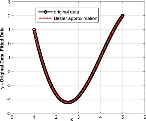
A second-order Bessel differential equation was solved using known boundary conditions. The data were created at 200 points using MATLAB Bessel functions of the first kind. Figure 6 represents the data at 200 points. In all the figures, the original discrete data are represented by the round symbol ‘o’ to suggest discreteness. Since the initial data are smooth, the number of data points is excessive but was done to increase the LSE.

Figure 6. Example 1: data approximation using Bezier function.

Figure 6 also provides the comparison of the original data and the data approximated by a Bezier function. The order of the best Bezier function is 14. The data statistics included minimum, maximum, mean, quartiles, median, variance, standard deviation, skew and kurtosis. The statistics for both the x and y data matched at least to the fifth place after the decimal and is not reported here. The average absolute error per point for the y data was 3.63608e–007. The figure indicates that the original data and the Bezier approximation match up very well visually. The order of the fit was independent of the number of data points. The average error was of the similar magnitude. It was checked by varying the number of points between 20 and 200. It is necessary that the data points include features over the entire domain.

4.1.1. Bezier coefficients

The x and y Bezier coefficients for Example 1 are

Once the coefficients are known, the various derivatives can be obtained through the application of chain rule.

4.1.2. Boundary conditions

The information about the boundary conditions is an important feature of technique. The boundary conditions for the original data and the Bezier approximation is compared in Table 1. Only conditions on x and y were required to generate the data. The derivative information was not required and therefore is marked as not given. The table indicates that additional derivative information can be obtained if needed.

Table 1. Example 1: comparison of the boundary conditions.

Type	Original data	Bezier data
x (initial)	1	1
x (final)	5	5
y (initial)	1	1
y (final)	2	2
dy/dx (initial)	Not given	−7.2728
dy/dx (final)	Not given	2.1184
d^2y/dx^2 (initial)	Not given	6.5163

The next step is to identify the specific form of the differential equation.

4.1.3. First generic form of the differential equation

A variable coefficient linear ODE form in (12) was assumed.

In all the generic forms, there is an expectation that if the exponent (or the highest exponent) is 0, then the entire term is dropped from residual computation. In this linear form, the exponents are chosen from the set of two values, 0 or 1. The coefficients e₁, e₂, e₃, f₁, f₂, f₃, g₁, g₂, g₃, h₂, h₃ belong to the set [−1 0 1]. The coefficient h₁ will belong to the set [−1 −0.75 −0.5 −0.25 0 0.25 0.5 0.75 1]. These choices are governed by two factors. The first is to keep the computation time small. The second is based on the known form of the solution. Note that the derivatives in the expression are the derivatives of the Bezier function, which is evaluated prior to this phase of calculations. Array programming is used for the computations.

4.1.3.1. Solution by exhaustive enumeration

An LSE formulation of the type in (14) is constructed for the generic form in (12). In all the solutions presented, the appropriate LSE was less than 1.0e–08. The number of loops executed was 22,497,279 and the time required was 871 s of CPU time.

The solutions for the exponents are: a₁ = 0, b₁ = 1, c₁ = 1, d₁ = 1.

The polynomial coefficients are: e₁ = 1, e₂ = 1, e₃ = 1, f₁ = 0, f₂ = 0, f₃ = 1, g₁ = 0, g₂ = 1, g₃ = 0, h₁ = −0.25, h₂ = 0, h₃ = 1. Substituting in the generic form (12), the differential equation can be assembled as (16)

This exactly matches the differential equation that was used to create the data in Figure 6. The procedure in this article has identified the exact form of the equation and also matched the boundary conditions (Table 1).

4.1.4. Second generic form of a differential equation

Here, the variable coefficient nonlinear generic form of ODE (13) is used

The exponents can be 0, 1 or 2. The unknowns in the coefficient terms are mostly selected from three discrete values [−1, 0, 1], while only the coefficient h₁ will belong to the set [−1, −0.75, −0.5, −0.25, 0, 0.25, 0.5, 0.75, 1]. The set of discrete variables was limited by consideration of computational time.

4.1.4.1. Solution by exhaustive enumeration

An LSE equation similar to (14) is constructed for this generic form and used to drive the optimization.

The solution for the exponents is a₁ = 0, a₂ = 1, a₃ = 1, a₄ = 1, b₁ = 1, b₂ = 0, b₃ = 0, c₁ = 1, c₂ = 0, d₁ = 1.

The coefficients are e₁ = 1, e₂ = 1, e₃ = 1, f₁ = 0, f₂ = 0, f₃ = 1, g₁ = 0, g₂ = 1, g₃ = 0, h₁ = −0.25, h₂ = 0, h₃ = 1.

Substituting this information in the generic form and dropping the entire term if the exponent of the highest derivative is 0, the enumeration yields the correct form of the differential equation (16).

This is the ODE used to establish the discrete data. The linear differential equation is identified even though the generic form is built to capture nonlinearity. The time for computation was around 3.06e04 CPU seconds, which is about 8.5 h on the SMP machine.

4.1.4.2. Solution through heuristic enumeration

The heuristic enumeration allows us to increase the set of discrete variables for all of the coefficients. The generic form in (13) was once again chosen. All coefficient unknowns could belong to one of nine discrete values that were associated with h₁. The exhaustive enumeration would take several weeks. The heuristic enumeration was run for a robust 1 billion cycles. It also identified the correct form of the ODE. It required 28.3 h of CPU time on the SMP machine.

4.2. Example 2: discovering the Blasius equation

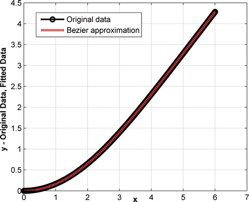
The Blasius equation, a nonlinear ODE, describing laminar flow over a flat plate, is numerically solved to create the data for this example. The actual equation describes a two-point BVP. The integration is over a finite limit as the solution becomes quickly asymptotic. Figure 7 shows the plot of the discrete data for Example 2.

Figure 7. Example 2: data approximation by Bezier function.

Figure 7 also shows the comparison of the original data and the Bezier approximation. It visually indicates that the quality of approximation is excellent. This conclusion is also backed by two-dimensional data statistics for both the x and y data. They agree to at least the fifth decimal place and are not reported here. The best order of the Bezier function is 12. There were 101 data points. The number of data points did not affect the order. The average absolute error per point was 8.81512e–007.

4.2.1. Bezier coefficients

The Bezier function coefficients are:

Once the coefficients are known, the various derivatives required for the generic differential equation can be easily obtained by the application of chain rule. They were calculated prior to the Step 2 of the procedure to identify the exact form of the ODE.

4.2.2. Boundary conditions

The boundary conditions for the original data and the Bezier approximation are compared in Table 2. For this example, the derivative information at the boundaries is required to generate the original data. The Bezier approximation is unaware of the derivative information. The derivative information in the table is extracted after the Bezier function has been identified. There is close match of the first derivatives at the boundaries. The second derivative information provided in the table is often used to solve the Blasius equation as an initial value problem instead of a BVP. It indicates that the Bezier function is also able to match the second derivatives at the starting boundary. This table suggests that we have realized one of the requirements in the problem statement – discover the boundary conditions for the differential equation.

Table 2. Example 2: comparison of the boundary conditions.

Type	Original data	Bezier data
x (initial)	0	1.3234e–013
x (final)	6	6.0000
y (initial)	0	1.9390e–007
dy/dx (initial)	0	−1.3919e–005
dy/dx (final)	1	1.0001
d^2y/dx^2 (initial)	0.3326	0.3329

The next step is to identify the specific form of the ODE.

4.2.3. Solution by exhaustive enumeration

Like Example 1, this example was also successively solved using the constant coefficient (11) and the variable coefficient (13) nonlinear generic forms of the ODE, though only the former is included below. It was also solved through heuristic enumeration. The major difference was the time of computation. The ODE is rewritten with different coefficient symbols in (17). The exponents are all integers. They can be one of three values 0, 1 or 2. The unknowns in the coefficient terms are mostly selected from two discrete values [0.5, 1]. Once more, the particular set of discrete variables was chosen to limit computational time. (17)

The LSE equation (14) was used to recognize the specific form of the ODE.

The solutions for the exponents are a₁ = 1, a₂ = 1, a₃ = 2, a₄ = 0, b₁ = 2, b₂ = 2, b₃ = 1, c₁ = 0, c₂ = 0, d₁ = 0.

The solutions for the coefficients are: e₁ = 1, e₂ = 0.5, e₃ = 0.5, e₄ = 0.5.

Substituting this information in the generic form and dropping the entire term if the exponent of the highest derivative is 0, the enumeration yields the differential equation:

This is the Blasius equation used to generate the data. The CPU time for this investigation was 1.24e05 s or 34 h on a P4 machine. The number of evaluation cycles was 944,784.

4.2.4. Solution using global search

The GA from the Genetic Algorithm and Direct Search Toolbox from MATLAB was used to successfully identify the form of the ODE and the boundary conditions. This is still a two-step approach and Step 1 is still the same as in the previous implementation. For Step 2, the ODE was represented by the constant nonlinear generic form (17). Two error equations were also tested. The first is the LSE error in (14). The second is a new error criteria based on the sum of the absolute value of the residuals. The absolute error was equally effective in identifying the specific form of the ODE.

The genome was a vector of real numbers of the exponents followed by the coefficients. The implementation required custom functions for the creation of the genome, the fitness function, the mutation of the genome and the crossover function. The fitness function was the sum of the absolute value of the residuals over several points on the trajectory. The fitness function was penalized by adding a large constant if the trivial solution was detected. The mutation was a simple change in one of the variables selected randomly. The crossover function exchanged a random length of contiguous variables between two parents. Twenty per cent of the crossover genomes were generated as immigrants. The unknown exponents and coefficients were generated from the following relations: (18) (19) where cvalue represents a vector of 16 values and ceil, int8, rand are MATLAB functions. The coefficients can be one of 16 values between –2 and 2. (20)

This is a larger set than that used in exhaustive enumeration.

The solutions for the genome are [1, 1, 2, 0, 2, 2, 1, 0, 2, 0, −0.5, −0.25, 0.25, 0].

The solutions for the exponents are a₁ = 1, a₂ = 1, a₃ = 2, a₄ = 0, b₁ = 2, b₂ = 2, b₃ = 1, c₁ = 0, c₂ = 2, d₁ = 0.

The solutions for the coefficients are e₁ = −0.5, e₂ = −0.25, e₃ = 0.25, e₄ = 0.

The population size was 500. The number of generations was 1000. The mutation and crossover parameters were set to default values. The execution time was 210 s for 1000 generations on a P4 machine. The sum of absolute residuals was 2.4985e–04. The solution had stalled at this value. The form of the ODE was (21)

This is the exact form of the differential equation in Example 2. The global optimization approach ensures a better alternative to enumeration. It allows a larger set of discrete values with a modest time of computation. It should be remembered that the global solution is the trivial solution and is not acceptable. A simple penalization of the global solution will move it to neighbouring non-trivial solution. There are multiple solutions that yield the same exact form of the ODE in Equation (20).

5. Conclusions and future work

The inverse BVP dealing with homogeneous ODE is solved in two steps. In the first step, a Bezier function approximates the data. This step identifies the boundary conditions as well as the derivatives of the function over the range of the independent variable. In the second step, an error formulation based on a generic form of the differential equation is used to identify the unknown exponents and coefficients that will determine the specific form of the ODE.

The nature of the computations involved is very simple but the traditional error formulation will lead to trivial solution for the variables that identify the actual form of the ODE. This article makes the case for discrete computation. The global solution is the unacceptable trivial solution and must be penalized. This article solves the problem using direct and heuristic enumeration where the time for computation for even a small set of discrete values for the variables is immense and unacceptable.

To permit a larger set of discrete values and reduce the time for computation, it is necessary to explore discrete global search methods. In this article, a solution using the GA from MATLAB toolbox is also presented. This requires modest time for solution with a larger set of discrete values. This time is orders of magnitude less than enumeration and maybe the way forward to solve coupled ODE and PDE. The formulation is also very convenient for parallel computation.

While the Bezier function lies within the convex hull determined by the vertices and is also invariant under an affine transformation, the procedure in this article is based on smooth exact data. Data from experiments are not very smooth. Can these data identify a differential equation? Is preprocessing necessary to smooth the data before the technique in this article can be applied? These are important questions that have to be investigated. The uniqueness of the differential form obtained, the quality of the discrete data, the extent of the original data and the guaranteed success of this approach are important issues that needs to be examined in the future. If the global search can accommodate more variables as well as more values for variables, then it is important to identify a universal generic form that can be useful for practical problems.

References

- Cheney, M, 1997. Inverse boundary-value problems, Am. Sci. 85 (1997), pp. 448–455.
- Martin, TJ, and Dulikravich, GS, 1996. Inverse determination of boundary conditions and sources in steady heat conduction with heat generation, J. Heat Transfer 118 (1996), pp. 546–554.
- Shih-Yu, S, 1999. A numerical study of inverse heat conduction problems, Comput. Math. Appl. 38 (1999), pp. 173–188.
- Kurt, B, and Caudill, LF, 1996. An inverse problem in thermal imaging, SIAM J. Appl. Math. 56 (1996), pp. 715–735.
- G.S. Dulikravich, J.M. Thomas, and B.H. Dennis, Multidisciplinary Inverse Problems, Proceedings of the Inverse Problems in Engineering, Theory and Practice, 3rd International Conference on Inverse Problem in Engineering, WA, USA, June 13–18, 1999..
- P. Venkataraman, Inverse Airfoil Design using Design Optimization, Paper no. 96-2503, 14th AIAA Applied Aerodynamics Conference, New Orleans, LA, June 1996..
- B.H. Dennis, A Least-Squares Finite Element Formulation for Inverse Detection of Unknown Boundary Conditions in Steady Heat Conduction, DETC2008-49653, ASME 28th Computers and Information in Engineering Conference, Brooklyn, NY, 2008..
- Tadi, M, 2000. Evaluation of a two-dimensional conductivity function based on boundary measurements, J. Heat Transfer 122 (2000), pp. 367–371.
- Martin, TJ, and Dulikravich, GS, 1998. Inverse determination of steady heat convection coefficient distributions, ASME J. Heat Transfer 120 (1998), pp. 328–334.
- Loulou, T, 2007. Combined parameter and function estimation with applications to thermal conductivity, J. Heat Transfer 129 (2007), pp. 1309–1320.
- Monde, M, and Mitsutake, Y, 2001. A new estimate of thermal diffusivity using analytical inverse solution for one-dimensional heat conduction, Int. J. Heat Mass Transfer 44 (2001), pp. 3169–3177.
- A.M. Hernandez, G.S. Dulikravich, S. Blower, M.J. Colaco, and R.J. Moral, Identification of Parameters in a System of Differential Equations Modeling Evolution of Infectious Diseases, DETC2008-49595, 28th ASME Computers and Information in Engineering Conference, Brooklyn, NY, 2008..
- Woodfield, PL, Monde, M, and Mitsutake, Y, 2006. Improved analytical solution for inverse heat conduction problems on thermally thick and semi-infinite solids, Int. J. Heat Mass Transfer 49 (2006), pp. 2864–2876.
- Dennis, BH, Dulikravich, GS, and Yoshimura, S, 2004. A finite element formulation for the determination of unknown boundary conditions for 3D steady thermoelastic problems, ASME J. Heat Transfer 126 (2004), pp. 110–118.
- Wang, J, and Zabaras, N, 2004. A Bayesian inference approach to the inverse heat conduction problem, Int. J. Heat Mass Transfer 47 (2004), pp. 3927–3941.
- Deng, S, and Hwang, Y, 2006. Applying neural networks to the solution of forward and inverse heat conduction problems, Int. J. Heat Mass Transfer 49 (2006), pp. 4732–4750.
- P. Venkataraman, Explicit solutions for differential equation, Available at http://people.rit.edu/pnveme/ExplictSolutions2/index.html.
- P. Venkataraman, A New Class of Analytical Solutions to Nonlinear Boundary Value Problems, DETC2005-84604, 25th Computers and Information in Engineering (CIE) Conference, Long Beach, CA, September, 2005..
- P. Venkataraman and J.G. Michopoulos, Explicit Solutions for Nonlinear Partial Differential Equations using Bezier Functions, DETC2007-35439, 27th Computers and Information in Engineering (CIE) Conference, Las Vegas, NA, September, 2007..
- P. Venkataraman, One and Two Dimensional Data Handling using Bezier Functions, DETC2008-49101, 28th Computers and Information in Engineering (CIE) Conference, Brooklyn, NY, August, 2008..
- P. Bezier, How Renault uses numerical control for car body design and tooling, SAE Paper no. 680010, Society of Automotive Engineers’ Congress, Detroit, MI, 1968..
- Rogers, DF, and Adams, JA, 1990. Mathematical Elements for Computer Graphics, . London: McGraw-Hill; 1990.
- Gordon, WJ, and Riesenfeld, RF, 1974. Bernstein-Bezier methods for the computer-aided design of free form curves and surfaces, J. ACM 21 (2) (1974), pp. 293–310.
- Venkataraman, P, 2009. Applied Optimization with MATLAB Programming, . New York: John Wiley; 2009.