Identification of electromagnetic field parameters assuring the cancer destruction during hyperthermia treatment

Abstract

Electromagnetic field induced by two external electrodes and temperature field resulting from electrode action in the domain of biological tissue being a composition of healthy region and a tumour is considered. To warrant the optimum conditions of tumour destruction, the magnetic nanoparticles are embedded in this region. It is assumed that the temperature which assures an effect of destruction should be higher than 42°C. In this article, the problems relating to the electrodes’ electric potential identification and the simultaneous identification of potential and number of nanoparticles introduced to the tumour region are discussed. Additional information necessary to solve the task results from the postulated temperature inside the tumour region assuring its destruction. The problem has been solved using both the gradient method and evolutionary algorithm. The boundary element method is applied to solve the coupled problem connected with the heating of biological tissues.

Keywords:

• bioheat transfer
• electromagnetic field
• hyperthermia
• boundary element method

1. Introduction

Hyperthermia (42–46°C) is a condition which occurs when the body produces or absorbs more heat than it can dissipate. It is usually due to excessive exposure to heat. Hyperthermia can also be created artificially by medical devices and it may be used as a therapeutic method to obtain an artificial increase in temperature of certain types of cancer tissue, such as skin cancer 1. It has been well established that temperature above 42°C will cause necrosis of living cells. A very important problem is applying the heat directly to the tumour region in order to avoid the damage of healthy tissue surrounding this domain. Great efforts have recently been made to use magnetic nanoparticles for the concentrated heat deposition at the tumour region located inside the human body. The particles should be made from the material assuring the appropriate magnetic properties and biological compatibility. Here, the iron oxides magnetite (Fe₃O₄) and maghemite (γ-Fe₂O₃) can be applied 2. It should be pointed out that the injection of nanoparticles to the human body belongs, most certainly, to the group of invasive interventions, but on the other hand, the effectiveness and precision of heating operation are essentially better than in the case of a procedure neglecting the particle injection.

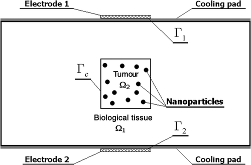
In this article, a simplified 2-D electromagnetic and temperature fields induced by two external electrodes in the biological tissue containing a tumour with magnetic nanoparticles (Figure 1) are considered. The aim of our investigations is to determine the electric potential of the electrodes relative to the ground assuring the temperature at the nodes located in the tumour region greater than the border temperature. The more complex task concerns the simultaneous identification of electric potential and the number of particles introduced to a tumour region. To solve the problems formulated, the evolutionary algorithm and gradient method coupled with the boundary element method 3 have been applied. In the final part of this article, the examples of computations are presented.

Figure 1. Hyperthermia system.

2. Electromagnetic field

Because the wavelength of the radio frequency (RF) current in tissues is much greater that depth of a human body, the quasistatic electric field approximation can be applied. The quasistatic electric field is irrotational, so the electric potential can be introduced. The potential inside the healthy tissue (e = 1) and tumour region (e = 2) is described by the system of Laplace equations (1) where ε_e (C² N⁻¹ m⁻²) is the dielectric permittivity of sub-domains Ω_e. At the interface Γ_c of the tumour and healthy tissue (Figure 1) the ideal electric contact is assumed to be (2)

On the external surface of tissue coming in contact with the electrodes, the following condition is given: (3) where U [V] is the electric potential of the electrode relative to the ground. On the remaining external boundary of tissue, the ideal electric isolation is assumed to be

The electric field inside the tissue is determined by equation (4)

Heat generation Q₁ (W m⁻³) due to the electromagnetic dissipated power in healthy tissue depends on the conductivity σ₁ (S m⁻¹) and the electric field E₁ 2 (5)

The tumour region with embedded magnetic particles is treated as a composite and due to the assumed homogeneity of Ω₂, the mean value of electrical conductivity σ₂ of this sub-domain can be approximated as , where are the electrical conductivities of the tumour and the particles, respectively, and is the concentration of particles (n is the number of particles, r is the radius of particle, and P_t is the tumour area – 2-D problem is considered here).

The amplitude of the magnetic field intensity can be expressed as 2 (6) where μ₀ = 4π × 10⁻⁷ Tm A⁻¹ is the dielectric constant permeability of free space, f (Hz) is the frequency of electromagnetic field, R (m) is the radius of the magnetic induction loop, N(χ) is the demagnetizing factor (N(χ) = 1/3 for a spherical composite), and χ (here: χ = χ′ + iχ″ 1) is the susceptibility of the magnetic nanoparticles.

Heat generation by superparamagnetism (SPM) is given by 2 (7) and then for one has (8)

3. Temperature field

The temperature field in the healthy tissue and the tumour region with embedded magnetic nanoparticles is described with the system of Pennes equations 2–4 (9) where e = 1 and e = 2 correspond to the healthy tissue and tumour regions, respectively, T_e is the temperature, λ_e W mK⁻¹ is the thermal conductivity, k_e = G_Bec_B (where G_Be (1 s⁻¹) is the perfusion rate, c_B J m⁻³ K is the volumetric specific heat of blood), T_B is the supplying arterial blood temperature, Q_met e (W m⁻³) is the metabolic heat source and Q_e(x, y) (W m⁻³) is the heat source connected with the electromagnetic field action. It should be noted that thermal conductivity λ₂ of tumour region with nanoparticles can be calculated as follows: , where are the thermal conductivities of tumour and nanoparticles, respectively.

At the interface Γ_c between the tumour and healthy tissue, the ideal contact is assumed to be (10)

On the upper and lower surfaces of the healthy tissue domain (skin surface), the convection condition is taken into account: (11) where α_w W m⁻² K is the heat transfer coefficient between the skin surface and the cooling water and T_w is the cooling water temperature. On the remaining boundaries, the adiabatic condition can be taken into account. This condition results from the consideration that at the positions far from the centre of the domain, the temperature field is almost not affected by the external heating 2.

4. Inverse problem

The first inverse problem which will be discussed consists of the identification of electric potential U of the electrodes under the assumption that the mean temperature in the tumour region is equal to T_h and the temperature field in the sub-domain considered is an uniform one. The final temperature field inside the tumour corresponding to the optimum value of identified parameter is heterogeneous, of course. The following criterion is considered: (12) where T_i is the nodal temperature located inside the tumour and resulting from numerical solution of direct boundary problem for assumed value of potential U.

In the case of gradient method application 5, the function is expanded in a Taylor series about known value of parameter U (13) where is the calculated temperature under the assumption that U = U^k. It should be pointed out that U⁰ is an arbitrary assumed value of variable U (for k > 0 it results from the previous iteration).

Substituting (13) into (12) and using the necessary condition of minimum, one obtains the following formula which allows one to determine in an iterative way the new value of identified parameter (14) where is the sensitivity coefficient, while k is the number of iteration. The sensitivity model has been constructed here using the direct approach 5,6 consisting of differentiation of governing equations with respect to parameter U. The iteration process is stopped when k = K, where K is the assumed number of iterations or when the predefined value of the criterion (12) is achieved.

The same criterion (12) is used in the case of simultaneous identification of electric potential U and number of nanoparticles n. The formula corresponding to Equation (13) takes the form (15) where is the sensitivity coefficient with respect to n.

Substituting (15) into (12) and using the necessary condition of minimum, one obtains the following system of equations which allows for an iterative way to determine the new values of identified parameters: (16)

To identify the electric potential U and number of nanoparticles n, the evolutionary algorithm has been also applied 7,8. As in the case of gradient method application, the functional (12) should be minimized with respect to the unknown parameters. A chromosome (vector) characterizes the solution (17) where U and n are the genes containing information about the electric potential and number of nanoparticles, respectively.

The genes are the real numbers on which constrains are imposed in the form (18)

The evolutionary algorithm starts with an initial population. This population consists of S chromosomes p^s, s = 1, 2, … , S, generated in a random way. Every gene is taken from the feasible domain. For the assumed values of p^s, s = 1, 2, … , S, the direct problems described by Equations (1)–(3) and (9)–(11) are solved by means of the boundary element method. The next stage is an evaluation of the fitness function (12) for every chromosome p^s and the selection is employed. The selection is performed in the form of ranking selection or the tournament selection 8 and the evolutionary operators, mutation, crossover, and cloning are applied. In this way, the next population is created. The process is repeated until the chromosome, for which the value of the fitness function is zero, is found or after the achieving the assumed number of generations.

In evolutionary computations, the following evolutionary operators are applied 7,8:

•	uniform mutation operator – which creates the gene values in chromosome by choosing new ones in random way,
•	nonuniform mutation operator – which creates the gene values in chromosome using the Gauss distribution, the amplitude of such mutation in each generation is equal where pop is the number of generation,
•	arithmetic crossover operator – which creates the new chromosome with genes which are linear combination of two randomly chosen chromosomes, the weight of linear combination is generated randomly,
•	cloning operator – which makes possible the passage of the best chromosome to the next population without necessity of participation in the process of selection.

In Table 1, the parameters of evolutionary algorithm used in computations are collected.

Table 1. Evolutionary algorithm parameters.

Number of generations	Number of chromosomes	Probability of uniform mutation	Probability of nonuniform mutation	Probability of arithmetic crossover	Probability of cloning
100	50	30%	20%	60%	10%

5. Boundary element method

The direct problems and in the case of gradient method the sensitivity problems have been solved by means of the boundary element method 4,9,10. So, the boundary integral equations corresponding to the equations (1) can be expressed as (19) where is the observation point; the coefficient is dependent on the location of source point , . For domain Ω₁, the boundary Γ corresponds to the external and internal boundaries of the healthy tissue; for domain Ω₂, the boundary Γ denotes Γ_c. The fundamental solution of the problem discussed has the following form: (20) where r is the distance between points and (x, y). Differentiating the function with respect to the outward normal , the function is obtained: (21) where (22)

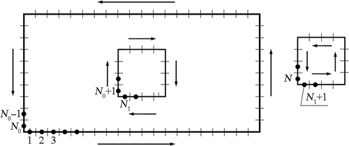
The boundaries of the domains are divided into N₁ and N₂ boundary elements, respectively, as shown in Figure 2.

Figure 2. Boundary elements and nodes.

For constant boundary elements 9,10, one obtains the following approximation of Equation (19):

•	for healthy tissue

(23)

•	for tumour region

(24) where (25) and (26) while .

The boundary condition (2) on the contact surface (healthy tissue – tumour region) written in the form (27) is introduced to the systems of equations (23) and (24). So, one obtains (28) and (29)

Joining together the systems of equations (28) and (29) and using the matrix convention, one has (30)

Next, the remaining boundary conditions (3) and should be introduced to the system of equations (30). This system allows one to determine the ‘missing’ boundary values of functions .

It should be pointed out that in order to determine the electric field inside tissue (Equation (4)), the partial derivatives , must be known. One of the possibilities is utilization of equations (19) for internal nodes and then (31) and (32)

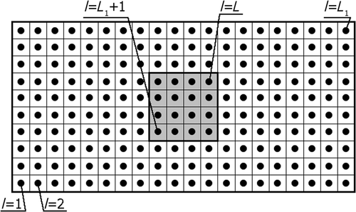
Applying previously presented discretization of the boundaries for the sub-domains, numerical calculations of partial derivatives are not difficult to obtain. These derivatives are determined at the internal nodes as shown in Figure 3.

Figure 3. Discretization of the sub-domains considered.

The Pennes equations (9) can be written in the form (33) where (34)

The boundary integral equations corresponding to the equations (33) can be expressed as follows: (35) where (36) and (37) while . In formulas (36) and (37), are the modified Bessel's functions of the second kind, and zero and first orders, respectively 9.

To solve Equations (35), not only the boundary but also the interior of the domains considered should be discretized, as shown in Figure 3.

For constant boundary elements and constant internal cells, one obtains the following systems of equations:

•	for healthy tissue (38)
•	for tumour region (39) where (40) and (41) while (42)

The systems of equations (38) and (39) are coupled by boundary condition (10), which can be written as (43)

Finally, one obtains (44)

The remaining boundary conditions should be introduced to the system of equations (44). The solution of (44) allows one to calculate the ‘missing’ boundary temperatures and heat fluxes . Next, the temperatures at the internal nodes can be calculated using adequate formulas 9,10.

In this article, the external boundary of the tissue has been divided into 60 constant boundary elements, the interface Γ_c of the tumour and tissue has been divided into 16 boundary elements. To solve the Pennes equation in the interiors of Ω₁ and Ω₂, the L₁ = 184 and L₂ = 16 nodes (internal cells) have been distinguished, respectively.

6. Results of computations

The rectangular domain of dimensions 0.08 m × 0.04 m has been considered. The heating area is described as {0.032 m≤ x ≤ 0.048 m, y = 0}, {0.032 m ≤ x ≤ 0.048 m, y = 0.04 m}, the tumour region corresponds to Ω₂ = {0.032 m ≤ x ≤ 0.048 m, 0.012 m≤ y ≤ 0.028 m} (Figure 1).

At first, the temperature distribution in the tissue with a tumour subjected to electric field action in the case of ‘natural’ situation (the particles are not introduced) has been considered. For healthy tissues, the following parameters have been assumed: thermal conductivity λ₁ = 0.5 Wm⁻¹ K⁻¹, perfusion rate  = 0.0005 1 s⁻¹, metabolic heat source  = 4200 Wm⁻³, blood temperature T_B = 37°C and volumetric specific heat of blood  = 4.2 MJ m⁻³ K⁻¹ 2. It has been revealed that the existence of malignant tumour often leads to a very different blood perfusion and abnormally high capacity of metabolic heat source in the tumour region 2,4. The following parameters are thus given for a highly vascularized tumour situated in the skin tissue:  = 0.002 1 s⁻¹,  = 42,000 Wm⁻³ and λ₂ = 0.6 Wm⁻¹ K⁻¹ 2. On the skin surface, the Robin boundary condition (Equation (11): α_w = 45 W m⁻² K⁻¹, T_w = 20°C) has been accepted.

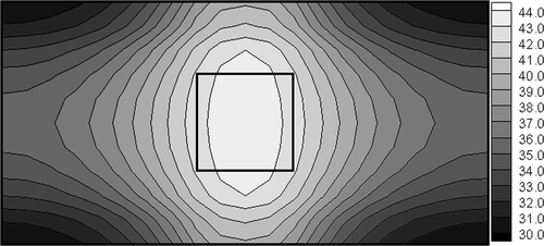
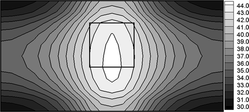
Additionally, it is assumed that the frequency of electromagnetic field is f = 1 MHz and the radius R of magnetic induction loop is 0.01 m. The following values of parameters have been used 2: electric conductivity of the healthy tissue σ₁ = 0.4 S m⁻¹, electric conductivity of the tumour region σ₂ = 0.6 S m⁻¹, dielectric permittivities ε₁ = 2000ε₀, and ε₂ = 2400ε₀ (ε₀ = 8.85 × 10⁻¹² C² Nm⁻²), respectively. The aim of computations is to determine the electric potential of electrodes assuring the minimum value of functional (12) for T_h = 43°C. In other words, the temperature in the domain of the tumour should be close to the postulated value of T_h. The results of computations obtained by gradient method corresponding to optimum value of U (U = 10.9 V, at the same time value of criterion (12) equals S = 1.45), are shown in Figure 4. The temperatures T_i at the nodal points corresponding to the tumour domain are from the scope (42.7, 43.3) and it assures the cancer's destruction.

Figure 4. Temperature distribution corresponding to U = 10.9 V, symmetrical position of tumour.

Unfortunately, the temperatures in the sub-domain of healthy tissue close to the tumour region are also higher than 42°C and this situation leads to the effects of undesirable destruction. The difficulties connected with the correct control of the process discussed increase when the tumour region is located asymmetrically in relation to external boundaries limiting the system. As an example, in Figure 5 the temperature distribution corresponding to the optimum value of U (U = 11.2V, S = 6.62, T_i ∈ (41.8, 43.9)) is shown.

Figure 5. Temperature distribution corresponding to U = 11.2 V, asymmetrical position of tumour.

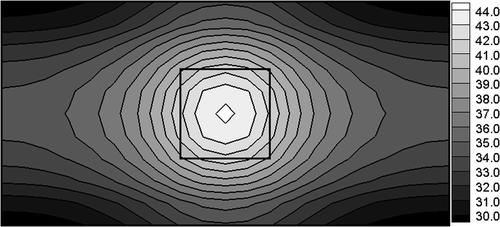
The better situation takes place when the nanoparticles are introduced to the tumour region. Here, we assume that the number of particles equals n = 10⁸, while r = 10 nm (10⁻⁸ m). The nanoparticles are made from iron oxides and maghemite γ-Fe₂O₃ whose electric conductivity equals ε₃ = 25,000 S m⁻¹, thermal conductivity λ₃ = 40 Wm⁻¹ K⁻¹, and χ″ = 18 2. As previously, the electric potential of electrodes U is identified and the remaining input data are the same. For the case considered, one obtains U = 5.24 V (S = 10.87). The temperature field for identified values of U is shown in Figure 6. One can see that the temperatures T_i > 42°C are located only in the tumour domain.

Figure 6. Temperature distribution (domain with nanoparticles) corresponding to U = 5.24 V.

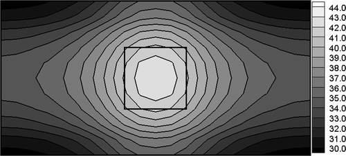
The last example concerns the simultaneous identification of particles number n and electric potential of electrodes U assuring the postulated temperature distribution in the tumour region. The optimum values of U and n (U = 8.017 V, n = 2.47 × 10⁷, which correspond to S = 6.04) have been found using the evolutionary algorithm. The temperature distribution for these values of identified parameters is shown in Figure 7.

Figure 7. Temperature distribution (domain with nanoparticles) corresponding to U = 8.017 V, n = 2.47 × 10⁷.

The same task has been solved again by means of gradient method. The postulate of uniform temperature inside the tumour (as previously) did not give good results (the problems of iterative process convergence). It turned out that assumption of a more realistic postulated temperature distribution in sub-domain (42°C close to the contact surface and 43°C inside ) entailed the essential improvement of algorithm efficiency; in particular, for the wide scope of sensible initial values U⁰, n⁰, the algorithm was convergent to the expected values of U and n; this means U = 9.1 V, n = 8.78 · 10⁸ (S = 1.28).

7. Conclusions

The proposed way of choice of the electric potential and also the nanoparticle number seems to be quite effective and sufficiently exact. It should be pointed out, however, that the method presented can assure the good results under the condition that the size and position of tumour region are exactly known. The optimum location of electrodes is also a priori assumed. Here, one can mention the identification algorithm which allows us to determine the size and position of tumour region on the basis of temperature distribution on the skin surface 11,12. It is well known that the apparition of tumour region leads to the increase of a local perfusion and capacity of metabolic heat source. So, the change of skin surface temperature can provide the essential information about the menace.

The results presented show that the ‘natural’ action of electromagnetic field does not assure the possibilities of heating control and the effect of healthy tissue destruction can appear. Quite a different situation takes place when the additional procedure consisting of the nanoparticle injection to the tumour region is introduced.

The solution of the inverse problem using gradient method seems to be quite satisfactory. The iterative procedure applied to determine the electric potential is convergent in spite of the considerable distance between the start point and the searched final value. In the case of simultaneous identification of electric potential U and number of nanoparticles n by means of the gradient method, the difficulties with the proper choice of initial values U and n appear and the iteration process is not always convergent. Introduction of nonuniform postulated temperature distribution in the domain of the tumour region allows one to avoid such a situation. The evolutionary algorithm is a time-consuming one and the error of identification is greater than in the case of gradient method application, but the solution of inverse problem consisting of the simultaneous identification of U and n can be always obtained.

Acknowledgement

This study was supported by grant no. N N501 3667 34 from the Polish Ministry of Education and Science.

References

- Wang, H, Dai, W, and Bejan, A, 2007. Optimal temperature distribution in a 3D triple-layered skin structure embedded with artery and vein vasculature and induced by electromagnetic radiation, Int. J. Heat Mass Transfer 50 (2007), pp. 1843–1854.
- Lv, YG, Deng, ZS, and Liu, J, 2005. 3D numerical study on the induced heating effects of embedded micro/nanoparticles on human body subject to external medical electromagnetic field, IEEE Trans. Nanobiosci. 4 (2005), pp. 284–294.
- Majchrzak, E, Dziatkiewicz, G, and Paruch, M, 2008. The modelling of heating a tissue subjected to external electromagnetic field, Acta Bioeng. Biomech. 10 (2008), pp. 29–37.
- Majchrzak, E, and Mochnacki, B, 2002. Analysis of thermal processes occurring in tissue with a tumor region using the BEM, J. Theor. Appl. Mech. 1 (2002), pp. 101–112.
- Kurpisz, K, and Nowak, AJ, 1995. Inverse Thermal Problems. Southampton, Boston: Computational Mechanics Publications; 1995.
- Kleiber, M, 1997. Parameter Sensitivity. Chichester: John Wiley & Sons Ltd.; 1997.
- Michalewicz, Z, 1996. Genetic Algorithms + Data Structures = Evolution Programs. Berlin: Springer-Verlag; 1996.
- Arabas, J, 2001. Lectures of Evolutionary Algorithms. Warsaw: WNT; 2001, (in Polish).
- Brebbia, CA, and Dominguez, J, 1992. Boundary Elements, An Introductory Course. London: Computational Mechanics Publications, McGraw-Hill Book Company; 1992.
- Majchrzak, E, 2001. Boundary Element Method in Heat Transfer. Czestochowa: Czestochowa University of Technology; 2001, (in Polish).
- Paruch, M, and Majchrzak, E, 2006. Numerical simulation of tumor region identification on the basis of skin surface temperature, Acta Bioeng. Biomech. 8 (2006), pp. 143–150.
- Paruch, M, and Majchrzak, E, 2007. Identification of tumor region parameters using evolutionary algorithm and multiple reciprocity boundary element method, Eng. Appl. Artif. Intell. 20 (2007), pp. 647–655.