Comparison of global and sequential methods for an inverse heat transfer problem

Abstract

This article presents a comparison between global and sequential methods to solve inverse problem related to the baking process. Both methods aim to reconstruct the wall temperature profile in the baking oven from the temperature of flux sensor (h-Monitor). The global method solves the adjoint and sensitivity equations to compute the gradient conjugate descent direction. This method contains regularization term that modifies the computation of the gradient. The sequential method computes at each time step a quasi-Newton descent direction taking into account a regularization term. This method may consider one-step or some time steps to improve the descent direction. The comparison shows that both methods perform well. However, the global method is better for noisy data and the sequential method provides satisfying results which makes it an interesting approach because of its simplicity.

Keywords:

• inverse methods
• heat transfer
• sequential method
• regularization
• global method

Nomenclature

A	=	differential operator
Ap	=	area of h-monitor
AT	=	linearized operator for T
	=	linearized operator for Tw
Cp	=	specific heat of h-monitor
e	=	h-monitor emissivity
ew	=	wall emissivity
G	=	gradient of the functional
h	=	heat transfer coefficient
i	=	experimental data index
J	=	performance index
k	=	iteration index
L	=	height
m	=	mass of h-monitor
N	=	number of experimental data
qc	=	total heat flux impinging of the solid block surface
s	=	descent search
t	=	time
T	=	h-monitor temperature
	=	measured temperature of h-monitor
Tw	=	wall temperature
Tc	=	solid block temperature

Greek symbols

α	=	regularization parameter
β	=	directional step
ΔT	=	sensitivity function
λ	=	adjoint variable
ε	=	optimization error tolerance
η	=	random variable
ρ	=	specific density
σ	=	variance
σB	=	Stephan–Boltzmann constant

Index

mod	=	model
reg	=	regularization
w	=	wall

1. Introduction

Inverse methods have been applied for the estimation of function or parameter in numerous heat transfer problems involved in thermal processes. For instance, parameters may be physical properties such as conductivity, heat transfer coefficients and emissivity. Functions could be thermal flux on the boundary of the domain or heat source intensity within the domain investigated. Inverse methods consist of a model describing the system and experimental data to identify unknown parameters or functions associated with the system under investigation. Inverse problems are generally ill-posed and the difficulties related to this property increase when the experimental data are noisy.

Industrial baking is a complex process involving heat and mass transfer combined with chemical reactions and product deformation. Typically a baking product is heated by radiation and convection heat transfer. The ceiling and the roof emit radiation flux to the product while convection results from the air stream circulating over the product. The quality of the baking product depends on the temperature profile of the product that is caused by combination of radiation and convection flux. When introducing a new baking product, it is important to evaluate the actual heat flux received by the product. To find the appropriate heat policy for a given baking product, information on the heat flux received by the product can be obtained via data acquisition system such as a h(heat)-monitor. To perform this task, the baking industry will use a pilot oven and a simplified product as h-monitor 1. The h-monitor data acquisition can be fast (up to one measurement per second) but temperature data are generally noisy.

Inverse methods can be applied to steady state or transient problems. For steady-state problems, inverse methods are relatively simple and generally involve minimization of the distance between the simulated results and the experimental data for sensor spatially dispersed. The minimization may be performed with the help of the gradient computation of the performance index (distance between simulation and experiments). The gradient of performance index is computed from the sensitivity function and the adjoint system. Hong et al. 2 have identified the wall temperature in a rectangular enclosure with radiation phenomena and natural convection. They used adjoint variables and took into account the momentum equation. They considered measurement errors with large variance (4 and 8 K), and the solution accuracy was severely deteriorated for some temperature profile. Chen and Yang 3 have identified the fouling layer profile in duct system with convection and conduction. The adjoint variables and sensitivity functions were used to compute the gradient. The fouling layer profile was accurately predicted except at the vicinity of the separation interface. The minimization may also be performed by the solution of the nonlinear system resulting from the discretization of the direct problem; in this case, the unknown variables comprise the unknown state variables and the unknown parameters. Nawrat and Skorek 4 successfully used this method to identify a thermal resistance for metal processing applications.

For transient problems, Gutierez Cabeza et al. 5 divide inverse methods into global methods and sequential methods. The global methods consider all experimental data available during the process while sequential methods consider only the data available at a given time step (and not data for the next time steps). The global methods use a global performance index representing the agreement between simulated results and experimental data for the entire duration of the process. Often, a regularization term is added to the performance index to address noise in the measurements. The global methods involve minimization of the global objective function (index + regularization term) with respect to the unknown parameters or functions. The minimization is performed with the computation of the adjoint system and sensitivity functions 6–8. However, the introduction of the adjoint system increases the complexity of the resolution because the adjoint system has the same dimension as the direct problem and solving the adjoint system requires integration from the final time to the initial time. To simplify the computation of the adjoint and gradient, Alestra et al. 8 consider analytical manual differentiation and automatic differentiation tools. Furthermore when the thermal process is combined with a fluid dynamic process, it is necessary to introduce the momentum equations which again increases the complexity of the mathematical formulation and the resolution method. Zhao et al. 9,10 develop global inverse methods to estimate thermal flux for thermo fluid processes which involves computation of the adjoint and sensitivity functions for the conservation, energy and laminar momentum equations. The thermal flux estimates were improved for flux with single frequency. However, high-frequency measurements noise significantly affect the quality of the results obtained with the inverse method. When the unknown parameters are constant (time and space), the adjoint functions are not necessary and the minimization may be performed with the sensitivity functions which simplifies the method 11–14.

The sequential methods are based on some measurements at each step. The unknown parameters and functions are computed at each step for the present and (some) previous times. These sequential methods have several similarities with on-line control and model predictive control methodology. For instance, Gutierez Cabeza et al. 5 use a sequential truncated singular value decomposition (SVD) approach for an inverse conduction problem to study the influence of two important parameters of this method: the number of future (sequential) measurements (the horizon) and the order of the truncation (model simplification). The truncated SVD method is a simplified version of the direct model and described the link between the input information (boundary conditions) and the output information (temperature). Results obtained by Gutierez Cabeza et al. 5 show that the sequential truncated SVD method is as good as the global SVD method and better in some cases. Girault et al. 15 use the sequential low-order model to solve an inverse heat transfer problem with convective and radiative boundary conditions for the estimation of the heat source; experimental data are used to obtain a low-order model for solving the inverse problem. Their results show how a low-order model was successful in finding accurate inverse solutions.

Recently, Cialkowski and Grysa 16 have combined global and sequential methods for an inverse heat conduction problem but their application was based on an analytical solution for the direct problem, which is only feasible for simple heat transfer problems.

Other studies have compared a variety of methods for solving inverse problems. Braga 17 compares two global methods, Tikhonov regularization and SVD, to solve inverse Fredholm integral and concluded that the SVD method is better than Tikhonov regularization. Chiwiakowski et al. 18 compare three global methods, Alifanov's approach, regularized solution based on entropy principle maximum with the quasi-Newton method and regularized solution with the genetic algorithm method. The numerical results show that the first two methods give better results for noisy measurements problems. Xu et al. 19 compare the direct inverse method, sequential observer-based method and optimization method for inverse heat problem. They conclude that the global optimization method (conjugate gradient method and regularization term) is the most accurate and the most robust but the most computationally intensive.

In this study, the global optimization method and the sequential optimization method will be compared for the identification of transient sources and simplified heat transfer problems encountered in the baking industry. The global method is efficient but complex and computational intensive whereas the sequential method is less complex but may be less accurate. The objective of this study is to compare the performance and the complexity of the global and sequential approaches for inverse problem resolution in order to know if a less complex method can provide satisfying results. The comparison will use criteria that estimate the distance between the model and the experimental data and the regularized form of the solution.

2. Baking problem

2.1. Direct problem

The complex tridimensional model which was investigated in this study was described previously by Boulet et al. 1. This model represents the baking operation of an inert product (h-monitor temperature acquisition system), by heated air recirculated in a pilot oven. The model takes into account conduction inside the inert product convection, and radiation heat transfer as well as turbulence in the oven. It is possible to derive a simplified model that gives acceptable results with respect to the complete model because the difference is less than 10%. The simplified model has the following assumptions:

•	The inert product has high conductivity; consequently, its temperature is assumed to be spatially uniform.
•	Turbulence effects are described by heat transfer coefficients.
•	Radiation flux is computed from the transient temperature of the oven walls.

Under these simplified assumptions, the energy balance of the simplified model corresponds to the following equation: (1) where T is the temperature of the h-monitor; T_w is the temperature of the wall; T_air is the constant temperature of the ambient air; h is the heat transfer coefficient between the h-monitor and the air; m and C_p are the mass and the specific heat of the h-monitor, respectively, e_w and e are the emissivity properties of the wall and the h-monitor and A_p is the area of the h-monitor. As the h-monitor is a cylinder with height L_H, Equation (1a) becomes: (2)

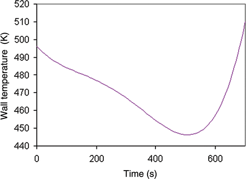
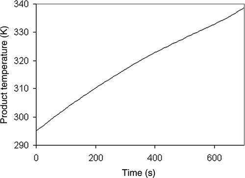
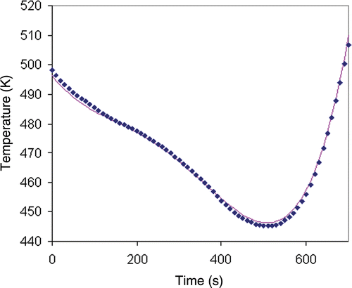
If the transient wall temperature is known, the direct problem computes the temperature of the h-monitor product. The exact values and for T_w and T are obtained from 1 and are shown in Figures 1 and 2.

Figure 1. Wall temperature for the baking of a muffin product.

Figure 2. Inert product temperature representing the baking of a muffin product.

2.2. Global method for the inverse problem

The inverse problem consists of estimating the wall temperature profile T_w(t) from transient temperature data of the h-monitor. The global method computes the wall temperature profile T_w(t) by minimization of the global index corresponding to the following functional: (3) (4) (5)

The first term of Equation (2), J_mod, is related to the quality of the model because it measures the distance between the model prediction and the experimental data. As the measurements are available at discrete times, the discrete norm will be used. The second term, J_reg, is the regularization term. The first-order regularization was selected in this application because previous studies have shown that better regularization was achieved than zero-order regularization 20. The parameter α is the regularization parameter and balances the weight between the model quality index, J_mod, and the regularization term J_reg. For industrial implementation, a smooth function for T_w(t) is required to meet physical constraints. With these assumptions, the functional has the following form: (6)

The variable N is the number of experimental data for different times t_i and with t_f the final time of the baking process.

The solution T_w is obtained by an iterative minimization procedure built on the gradient of the functional. There are several formal methods to obtain the gradient. In this study, the gradient is deduced from the adjoint system.

The state Equation (1) can be written as (7) where A is a differential operator and T and T_w are elements of functional space. The sensitivity equation of the state equation is: (8) where A_T and are the linearized forms of the operator A; ΔT and ΔT_w are the temperature sensitivity and the variation of the wall temperature. ΔT belongs to the same functional space as T and ΔT_w belongs to the same functional space as T_w. ΔT is solution of the linearized version of Equation (1) whereas ΔT_w is the forcing function. The linearization of Equation (1) gives: (9) The operators A_T and are defined by (10) (11) The adjoint system is defined by the following relation: (12) where (·, ·) is an inner product in a functional space, is the adjoint operator and λ is the adjoint variable. With functional spaces, the inner product is an integral and the boundary terms come from integration by parts and Green's theorem. If the state equation has regular initial (and boundary) condition and if the unknown parameters are not present in the initial (or boundary) conditions, the boundary terms of Equation (8) vanish and provide final (and boundary) conditions for the adjoint variable. For this study, the inner product is defined by and the adjoint operator is deduced from Equations (7a) and (7b): (13) Equation (3) can be transformed into an inner product: (14) The first variation of J(T_w) is: (15) If the first term of Equation (11) is identified to the first term of Equation (8), the following equation is obtained: (16) From Equations (9) and (12), the adjoint variable is defined by the following equation: (17) From Equations (5) and (11): (18) From Equation (7b), it follows that .

The gradient G(T_w) of the functional J(T_w) (Equation (3)) is defined from the first variation of the functional: (19)

The first term of Equation (14) has the form of Equation (15) whereas the second term does not explicitly contain the variation . The second term of Equation (14) may be rearranged by integration by parts and becomes: (20) From Equations (7b), (14) and (16), the first variation is expressed as

And consequently from Equation (15), the gradient G is defined by (21)

The stationary conditions give the differential equation for the minimum T_w(t): (22)

Equation (18) has the same form as presented by Akcelik et al. 21 who used Tikhonov regularization to identify diffusive source in convective diffusive transport equation. In the case of the global method, the direct and inverse problems are a two-point boundary value system. The temperature of the h-monitor and the derivative of the wall temperature are known at the initial time (t = 0) whereas the adjoint variable and the derivative of the temperature wall are known at the final time (t = t_f). Solving the two-point boundary values system is difficult. It is easier to solve the inverse problem by an iterative minimization approach. As the gradient of the functional is known, the common approach is the conjugate gradient method where the directional step is performed with the computation of the sensitivity function. The conjugate gradient descent search s^k has the following expression at the iteration k: (23) The new value of T_w is given by the following equation: (24)

The directional step β is obtained by the minimization of the performance index (Equation (3)) in the descent direction s^k. (25)

The minimization of the performance index with respect to directional step λ gives: (26)

The global method resolution approach (algorithm I) contains the following steps:

a.	Initial estimation for the wall temperature .
b.	Integrate the direct system (Equation (1)) from 0 to tf.
c.	Compute the index performance (Equation (3)) and stop if stopping criterion is met.
d.	Integrate the adjoint system (Equation (13)) and compute the gradient G (Equation (19)) from tf to 0.
e.	Compute the conjugate descent search s (Equation (19)).
f.	Integrate the sensitive system (Equation (6)) from 0 to tf and compute the directional step β (Equation (22)).
g.	Update the wall temperature Tw with Equation (20).
h.	Go back to step (b).

The stopping criterion is an important consideration for the inverse problem. As in optimization problems, the stopping criterion can be on the gradient of the functional; the optimization process stops when the norm of gradient is small (e.g. ).

The stopping criteria can also be related to the functional J_mod (Equation (2)) that measures the difference between the simulation and experimental values. For instance, the iterative process may stop when the index J_mod (Equation (2)) is smaller than a specified number (). With noisy product temperature measurements, the minimization stops when the model index J_mod is smaller than Nσ where σ is the variance of experimental data. The discrepancy principle 22 presents the inequality J_mod < Nσ as a condition specifying the allowed degree of proximity to the simulated and the experimental data. According to the principle of discrepancy, the optimization functional comprises only J_mod (no regularization term). With the inequality J_mod < Nσ, the conjugate gradient algorithm performs the regularization objective alleviating the computation of the exact irregular inverse solution. Alifanov et al. 23 use this approach to identify constant lumped parameters in radiative–convective heat transfer inverse problems. In this study, the complete index was minimized and did not involve the discrepancy principle.

If the previous termination tests fail, the minimization stops when two consecutive iterations did not result in sufficient decrease in the performance index or did not result in sufficient change in the successive T_w.

Broadly speaking, the direct and the inverse problems have no analytical solutions. Numerical methods such as finite differences, finite elements or finite volumes are required. In this study, the numerical integration method was Runge-Kutta 4. Furthermore, the computation of the performance index J and the computation of the gradient required the first derivatives and . These derivatives were approximated by the second-order approximation. For global methods, different time steps (1, 0.1, 0.01 s) have been tested and the results are not modified significantly. This behaviour is expected because the differential equations of direct problem and the sensitivity equations are stable with the forward integration and the differential equations of adjoints are stable with backward integration. The time step equal to 0.1 s was used to obtain an adequate discrete approximation of the continuous gradient.

Solving the inverse problem required a first estimate of the wall temperature and the numerical value for the regularization parameter α. The first guess for the wall temperature was available because the range of wall temperature for the baking process is known. In contrast, the appropriate value for the regularization parameter α is difficult to estimate. The solution has significant oscillations if the parameter α is too small and the gap between the model and experimental data increases if the parameter α is too large. The parameter α can be chosen by the L-curve technique 24 but this technique requires additional computation of the model quality index and regularization index. Han et al. 25 relate the regularization parameter to the variance error via the discrepancy principle but this approach requires the knowledge of the discretization error in the numerical schemes. Pereverzyev et al. 26 consider several regularization parameters and select the most appropriate according to quasi-optimality criterion. In this study, different values of regularization parameters were tested.

2.3. Sequential method for the inverse problem

For the investigated baking problem, the sequential approach obtains the unknown variable T_w at each time t, considering only a few measured and estimated temperatures of the h-monitor taken at time t and in the near future. As for the global approach, T_w was obtained by the minimization of functional comprising a term related to the quality of the model and a regularization term.

For sequential approach, the functional is: (27) where i = 1, … , N corresponds to the i experimental points, is the measurement at time t_i+1, T_w,i is the unknown wall temperature between t_i and t_i+1. The unknown T_w,i is assumed constant on the time range [t_i, t_i+1]. In Equation (23), the wall temperature T_w,i−1 is known and has been established at the previous step.

The derivative of the functional is given by (28)

The term is the sensitivity function related to the sensitivity ΔT defined previously in section 2.2. The sensitivity function is given by the following differential equation. (29)

Equation (25) is similar to Equation (6) that defines the differential equation for the sensitivity. The optimal value for T_w,i is the value for which the derivative (Equation (24)) is equal to zero. (30)

Equation (26), an implicit equation of T_w,i, was solved iteratively with the quasi-Newton method and the following iteration: (31)

The quasi-Newton method was used because the complete Newton method would require the second-order sensitivity function that has been neglected in our approach. This approximation is correct if the fit between the model and the experimental data is good. It is the same expression used in the Gauss–Newton method where the second derivatives of the objective function are approximated by the product of the sensitivity functions.

The sequential method resolution approach (algorithm II) has the following steps.

a.	Initial estimation of the wall temperature ; set i = 0.
b.	Set k = 0.
c.	Integrate the direct system (Equation (1)) from ti to ti+1.
d.	Compute the functional (Equation (23)); if termination criterion is respected, go to step (h).
e.	Integrate the sensitivity function system (Equation (25)) from ti to ti+1.
f.	Update the wall temperature with Equation (27).
g.	Set k = k + 1 and go to step (c).
h.	Set i = i + 1 and if i < N go to step (b).
i.	End.

The termination criterion is the same as for the global method. The initial estimate of the wall temperature is obtained from prior baking knowledge. The regularization parameter α has the same characteristics as the regularization parameter for the global approach. The differential equations (Equation (1a) and (9)) are solved numerically with the Runge-Kutta method. For sequential methods, different time steps (1, 0.1, 0.01 s) have been tested and the results are not modified. This behaviour is expected because the differential equations of direct problem and the sensitivity equations are stable with forward integration. The same time step as for the global method was used.

The sequential method can be modified, referred to as the horizon sequential method, considering several horizons to find . If p future temperatures are taken into account, the previous relationships are modified. Equation (23) becomes: (32) and Equation (27) becomes (33)

The value of p is generally small, to keep the method simple and the estimation accurate. In the case of the horizon sequential method, the algorithm is the same as the simple sequential method.

2.4. Direct problem and temperature experimental values

The direct problem considered in this study was investigated previously by Boulet et al. 1. They analysed the temperature profile of a specific baking product (muffin) represented as h-monitor in a pilot oven. The (exact) wall temperature profile and the corresponding h-monitor temperature for a t_f = 700 s baking process are presented in Figures 1 and 2.

The experimental product temperature data are the N points taken from Figure 2 for t_i = iΔt. In this study, the time step Δt was selected as 10 s and the number of experimental temperature data was N = 70. If the h-monitor temperature data (Figure 2) had no noise, the solution of the inverse problem corresponds to T_w profile shown in Figure 1. To evaluate the robustness of the global and sequential methods, noisy product data were tested. The noisy measurements were obtained by adding normal noise to the exact inert product temperature data (Figure 2). (34) where σ is the variance and η, the normal variable with mean equal to 0 and the variance equal to 1. For baking product, the variance σ is equal to 0.1 K.

3. Results

3.1. Inverse problem global method

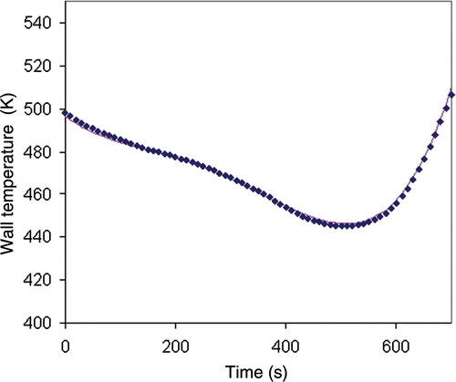
The wall temperature obtained by the global method and the exact h-monitor temperature data (no noise) is shown in Figure 3. The initial T_w estimate was 475 K and the regularization parameter was α = 0. In this case, the active criterion was the model quality index J_mod and the minimization process was stopped when the performance index was less than 10⁻³. The number of iterations was 23.

Figure 3. Wall temperature obtained by the global method (no regularization) for exact temperature data of the inert product solid line: exact solution; blue diamonds: inverse method solution.

The global method provided a wall temperature profile very close to the exact solution (Figure 3). Without regularization term (α = 0), the model index was J_mod = 2.2 × 10⁻⁵. The result shows that it is not necessary to introduce a regularization term when the h-monitor temperature data were without noise. When the regularization term was introduced, the results were also good (Figure 4) with regularization parameter α = 10⁻³. With the addition of a regularization term, the model quality index (J_mod = 0.017) was not as good as for the situation without regularization. The optimization process was stopped with the termination criterion on the gradient norm () corresponding to 64 iterations.

Figure 4. Wall temperature obtained by the global method (regularization) for exact temperature data of the inert product blue diamonds: inverse method solution; pink line: exact solution.

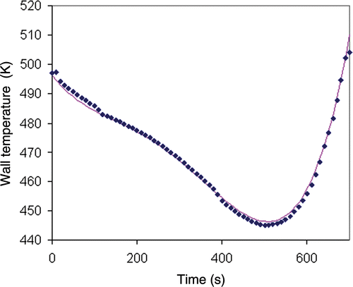
In both cases, most of the decrease in the objective function took place during the first five iterations. The profile of the wall temperature did not change significantly after 10 iterations. Figures 5 (without regularization) and 6 (with regularization) show the result of the global method for noisy inert product temperature data with variance σ = 1. As expected, the solution without regularization was not satisfactory (Figure 5) because the wall temperature profile is irregular. The active criterion termination was on the gradient while the model quality index was J_mod = 0.197. This result was reached after 70 iterations. The poor model quality index indicates that the wall temperature profile was quite different from the experimental wall temperature profile, which is not feasible in industrial implementation.

Figure 5. Wall temperature obtained by the global method (no regularization) for noisy inert product temperature data blue diamonds: inverse method solution; pink line: exact solution.

The estimated wall temperatures obtained with the global method and with regularization term (α = 5.0 × 10⁻³) showed good agreement with the exact solution in spite of the noisy inert product temperature measurements (Figure 6). The wall temperature profile was quite regular but still displayed some small-undesired variations. In this case, the active criterion termination was on the lack of improvement of the functional and the quality model index was J_mod = 0.328 for 32 iterations. Note that the minimization process converged only partially. A plateau was reached at this step where the functional remained stable. Probably, the calculation of the directional step β (Equation (22)) was not sufficient to ensure a decrease in the functional J. Table 1 shows that the global method gives adequate results for higher level of noise (σ = 0.2) as if the prediction are not as accurate as for the case of the lower lever.

Figure 6. Wall temperature obtained by the global method (weak regularization) for noisy inert product temperature data blue diamonds: inverse method solution; solid line: exact solution.

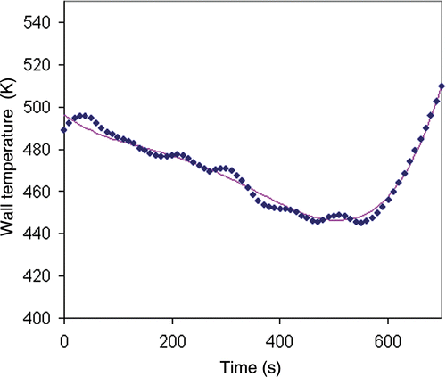
Table 1. Comparison for noisy (σ = 0.2) inert product temperature data.

Inverse method type and properties	Regularization index (Jreg)	Quality model index (Jmod)	Error	CPU times
Global method α = 0; p = 0	0	0.571	11.65	12
Global method α = 2 × 10^−2; p = 0	13.4 × 10^−2	0.848	3.12	5
Global method α = 4 × 10^−2; p = 0	23.3 × 10^−2	0.868	2.97	3.5
Global method α = 8 × 10^−2; p = 0	43.0 × 10^−2	0.879	2.82	3
Global method α = 10 × 10^−2; p = 0	43.3. 10^−2	0.93	3.06	3.5
Sequential method α = 0; p = 1	0	2.6 × 10^−3	47.3	1
Sequential method α = 2 × 10^−3; p = 5	3.2 × 10^−3	0.82	3.76	1
Sequential method α = 4 × 10^−3; p = 5	4.2 × 10^−3	0.99	3.27	1
Sequential method α = 4 × 10^−3; p = 3	4.1 × 10^−3	3.09	7.34	1
Sequential method α = 8 × 10^−3; p = 5	6.2 × 10^−3	1.78	4.62	1

If a very regular solution is desired, a larger value of the regularization parameter will be required. Figure 7 reports the solution for α = 8.0 × 10⁻². The agreement is good for most of the baking process except near the end where the boundary conditions () may distort the solution. However, the solution is uniform which is good for industrial implementation.

Figure 7. Wall temperature obtained by the global method (strong regularization) for noisy inert product temperature data blue diamonds: inverse method solution; pink line: exact solution.

3.2. Sequential method

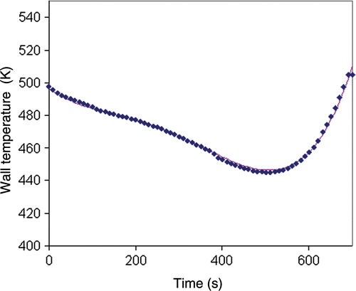
Figure 8 reports the estimates of the sequential method for the inert product temperature measurements with no noise. There is no regularization term (α = 0) and the horizon has one time step (p = 1). The agreement is very good when compared with the exact wall temperature profile. The criterion termination for the sequential optimization process (step d in algorithm II) was on the gradient norm (). The model quality index was J_mod = 10⁻⁸. The same results were obtained when higher horizons (p = 2, p = 3) were used.

Figure 8. Wall temperature obtained by the sequential method (no regularization; horizon p = 1) for exact inert product temperature data; blue diamonds: inverse method solution; solid line: exact solution.

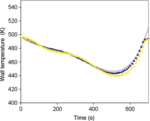
When the regularization term was included, it was important to increase the horizon when the regularization parameter became more significant. Figure 9 shows the effect of the horizon size with α = 10⁻³ as regularization parameter. With this value, the horizon size with p = 3, generated an adequate wall temperature profile whereas the horizon size p = 2 gave unsatisfactory results. The termination criterion was on the gradient norm and the model quality index J_mod was 0.293 (horizon p = 3). As expected, the addition of regularization term when the h-monitor temperature data were exact (no noise) did not improve the estimates.

Figure 9. Wall temperature obtained by the sequential method (regularization; horizon) for exact inert product temperature data; solid line: exact solution; yellow triangles: computed solution (horizon p = 2): blue diamonds: computed solution (horizon p = 3).

When experimental h-monitor temperature data were noisy, the estimates were quite different. Figure 10 reports the estimates of the sequential approach for noisy h-monitor temperature data with no regularization and horizon size, p = 1. If no regularization and horizon are considered (Figure 10), the wall temperature profile was inadequate even if the model quality index was very low (J_mod = 1.8 × 10⁻³). In addition, the estimated wall temperature profile is too irregular for industrial implementation. Figure 11 shows the profile obtained with the sequential method and the effect of the regularization parameter and the horizon size.

Figure 10. Wall temperature obtained by the sequential method (no regularization) for exact inert product temperature data; solid line: exact solution; blue diamonds: computed solution (horizon p = 1).

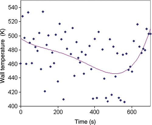
Figure 11. Wall temperature obtained by the sequential method (regularization; horizon) for noisy inert product temperature data; solid line: exact solution; yellow triangle: computed solution (horizon, p = 3 and α = 0.004); blue cross: computed solution (horizon, p = 5 and α = 0.002); blue diamonds: computed solution (horizon, p = 5 and α = 0.004).

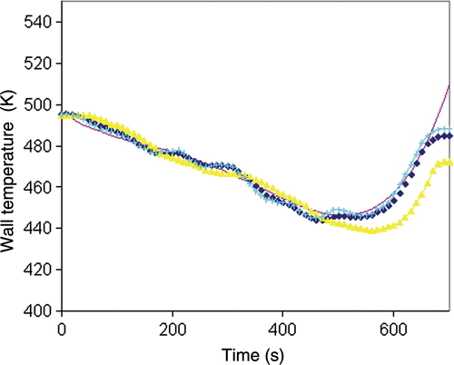
The sequential method generated the adequate wall temperature profile when the regularization term and horizon were included (Figure 11). In addition, the sequential method was more sensitive to the size of the horizon (p = 3 and p = 5, Figure 11) and less sensitive to the magnitude of the regularization parameter (α = 2 × 10⁻⁰³ and 4 × 10⁻⁰³, Figure 11). Table 1 shows that the sequential method gives adequate results for higher level of noise (σ = 0.2) as if the prediction are not as accurate as for the case of lower lever. For all situations investigated in this study, the agreement between the exact solution and the inverse solution was not very good near the end of the baking process. This gap is due to the size of the horizon that becomes smaller near the final time (algorithm II). For the inverse solution with horizon p = 5 and α = 4 × 10⁻⁰²³, the model quality index was J_mod = 1.01.

4. Discussion

Tables 2 and 3 summarize the performance of the global and sequential inverse problem methods when considering the exact and noisy h-monitor temperature data. The deviation of the estimated solution from the exact solution is computed by the function 14: (35)

Table 2. Method comparison for exact inert product temperature data.

Inverse method type and properties	Regularization index (Jreg)	Quality model index (Jmod)	Error	CPU times
Global method α = 0; p = 0	0	2.2 × 10^−5	0.967	6
Global method α = 10^−3; p = 0	5.1 × 10^−5	0.017	0.87	5.5
Global method α = 5 × 10^−3; p = 0	5.2 × 10^−3	0.072	0.98	6
Sequential method α = 0; p = 1	0	1.2 × 10^−8	0.84	1
Sequential method α = 10^−3; p = 2	3.8 × 10^−2	1.96	2.01	1
Sequential method α = 10^−3; p = 3	7.2 × 10^−3	0.293	1.75	1
Sequential method α = 2 × 10^−3; p = 3	27.2 × 10^−3	0.766	3.51	1

Table 3. Method comparison for noisy (σ = 0.1) inert product temperature data.

Inverse method type and properties	Regularization index (Jreg)	Quality model index (Jmod)	Error	CPU times
Global method α = 0; p = 0	0	0.197	6.01	6
Global method α = 5 × 10^−3; p = 0	6.9 × 10^−2	0.328	2.04	4
Global method α = 10 × 10^−3; p = 0	0.18	0.26	1.67	3.5
Global method α = 20 × 10^−3; p = 0	0.16	0.313	2.40	4
Sequential method α = 0; p = 1	0	1.8 × 10^−3	27.00	1
Sequential method α = 2 × 10^−3; p = 5	8.0 × 10^−2	0.55	2.55	1
Sequential method α = 4 × 10^−3; p = 5	4.2 × 10^−2	1.01	2.73	1
Sequential method α = 4 × 10^−3; p = 3	5.0 × 10^−2	5.98	6.57	1

Very accurate oven wall temperature profiles were obtained when the h-monitor temperature data were not noisy. As expected, the regularization term may be omitted. When the regularization term was included, the performance of the sequential method was improved when multiple horizons (p > 1) were introduced. For both methods, the quality index showed that the estimated wall temperature profiles gave the appropriate temperature of the h-monitor.

When considering noisy h-monitor temperature data, the two methods provided accurate estimates but required the addition of a regularization parameter (Table 3). The global method was better, considering the improved accuracy at the end of the baking process. The estimates with the sequential method improved as the horizon size increased.

An important difference between both the methods is their complexity. Algorithm I (global approach) required significant computations and data storage to perform complete iteration since each iteration requires a forward integration, a backward integration and a forward integration. The last integration (sensitivity equation) could be alleviated if the directional step β was not computed at each iteration. Tables 1–3 show that the relative CPU times for the global method are much more important than for the sequential method. If the direct problem is simple (consequently, the adjoint and sensitivity are also), the three integrations are not very computer or time consuming. When the direct problem is complex, powerful computational tools such as computational fluid dynamics (CFD) are required. The derivation of the adjoint system (and the sensitivity function system) can require time and the three integrations (with the associated storage of the variables) become time and computer consuming.

The sequential approach is simpler than the global method. Algorithm II does not require the adjoint system and consequently alleviates the backwards integration and the storage of the variables computed for the direct problem. This point is very important for complex systems, such as the turbulent Navier–Stokes equations. This is an important advantage of the sequential method. However, the sequential method requires the sensitive function system. The sensitivity function has the same complexity as the adjoint system but can be integrated with the direct problem. In addition, the sensitivity function system requires additional work. This additional work could be eliminated if numerical sensitivity functions are used instead of analytical ones. The numerical sensitivity function can be computed during the successive iterations of algorithm II.

The choice of the optimal parameter is an important step in any regularization method. The choice is related to the error criterion defined by Equation (31). This criterion measures the gap between the exact solution and the constructed solution by the inverse method. The optimal value of the regularization parameter corresponds to the minimum value of this criterion. Table 3 shows that the error is not very sensitive to the value of the regularization parameter for the global and sequential methods. Consequently, the range of the regularization parameter is quite large. The error criterion requires the exact solution of the inverse problem, generally unknown for industrial applications. In this case, the regularization term is an important element and can be related to industrial constraints. For an industrial oven, the heating power variation is physically limited. Consequently, the derivative term must be small to respect the technological limitations (0.8 K s⁻¹). The optimal value of the regularization parameter verifies this constraint.

5. Conclusion

The global and sequential inverse methods have been analysed and compared for solving inverse problem related to baking operations. The two methods use regularization term to obtain a smooth solution for the inverse problem. The two methods were successful in reconstructing the wall temperature profile from the exact and noisy h-monitor temperature data. For the situation with noisy inert product temperature data, the estimates with the global method were better than the sequential method because the global method gives a more regularized solution. However, the global method required the development and the computation of the adjoint system, which is a time-consuming computer-intensive task. The sequential approach is simpler and required only the estimation of the sensitivity. The multi-step version of the sequential approach gives a good solution for the inverse problem considered in this study and represents promising alternative to obtain good estimates for the solution of inverse problems of heat transfer baking applications.

Acknowledgements

The authors acknowledge Professor Nicolas Galanis for his valuable comments during this study. This project was carried out as part of the R&D program of the NSERC Chair in Industrial Energy Efficiency (chair holder: N. Galanis) established in 2006 at Université de Sherbrooke with the support of Hydro-Quebec (Energy Technology Laboratory, LTE), Rio Tinto/Alcan International Ltd. and the CANMET Energy Technology Center (CETC-Varennes, Natural Resources Canada).

References

- Boulet, M, Marcos, B, Dostie, M, and Moresoli, C, 2010. CFD modeling of heat transfer and flow field in a bakery pilot oven, J. Food Eng. 97 (2010), pp. 393–402.
- Hong, YK, Baek, SW, and Kim, YM, 2010. Inverse natural convection problem with radiation in rectangular enclosure, Numer. Heat Transfer, Part A 57 (2010), pp. 315–330.
- Chen, WL, and Yang, YC, 2010. Inverse estimation for unknown fouling-layer profiles with arbitrary geometries on the inner wall of a forced-convection duct, Int. J. Therm. Sci. 49 (2010), pp. 86–98.
- Nawrat, AJ, and Skorek, J, 2005. Inverse approach and sensitivity analysis for identification of ingot-mould thermal resistance in continuous casting of metals, Int. J. Comput. Fluid Dyn. 19 (6) (2005), pp. 429–436.
- Gutierez Cabeza, JM, García, JM, and Rodríguez, AC, 2005. A sequential algorithm of inverse heat conduction problems using singular value decomposition, Int. J. Therm. Sci. 44 (2005), pp. 235–244.
- Saker, LF, Orlande, HRB, Huang, C-H, Kanevce, GH, and Kanevce, LP, 2007. Simultaneous estimation of the spacewise and timewise variations of mass and heat transfer coefficients in drying, Inverse Prob. Sci. Eng. 15 (2) (2007), pp. 137–150.
- Yang, Y-C, 2007. Simultaneously estimating the contact heat and mass transfer coefficients in a double-layer hollow cylinder with interface resistance, Appl. Therm. Eng. 27 (2007), pp. 501–508.
- Alestra, S, Colinet, J, and Dubois, J, 2008. An inverse method for non linear ablative thermics with experimentation of automatic differentiation, J. Phys. Conf. Ser. 135 (2008), pp. 12003/1–12003/12.
- Zhao, F-Y, Liu, D, and Tang, G-F, 2009. Numerical determination of boundary heat fluxes in an enclosure dynamically with natural convection through Fletcher–Reeves gradient method, Comput. Fluids 38 (2009), pp. 797–809.
- Zhao, F-Y, Liu, D, and Tang, G-F, 2009. Inverse determination of boundary heat fluxes in a porous enclosure dynamically coupled with thermal transport, Chem. Eng. Sci. 64 (2009), pp. 1390–1403.
- Da Silva, CKF, Da Silva, ZE, and Mariani, VC, 2009. Determination of the diffusion coefficient of dry mushrooms using the inverse method, J. Food Eng. 95 (2009), pp. 1–10.
- Molavi, H, Pourshaban, I, Hakkaki-Fard, A, Molavi, M, Ayasoufi, A, and Rahman, RK, 2009. Inverse identification of thermal properties of charring ablators, Numer. Heat Transfer, Part B 56 (2009), pp. 478–501.
- Monteau, JY, 2008. Estimation of thermal conductivity of sandwich bread using an inverse method, J. Food Eng. 85 (2008), pp. 132–140.
- Lin, DTW, Yan, WM, and Li, HY, 2008. Inverse problem of unsteady conjugated forced convection in parallel plate channels, Int. J. Heat Mass Transfer 51 (2008), pp. 993–1002.
- Girault, M, Videcoq, E, and Petit, D, 2010. Estimation of time-varying heat sources through inversion of a low order model built with the modal identification method from in-situ temperature measurements, Int. J. Heat Mass Transfer 53 (2010), pp. 206–219.
- Cialkowski, M, and Grysa, K, 2010. A sequential and global method of solving an inverse problem of heat conduction equation, J. Theor. Appl. Mech. 48 (1) (2010), pp. 111–134.
- Braga, JP, 2001. Numerical comparison between Tikhonov regularization and singular value decomposition methods using the L curve criterion, J. Math. Chem. 29 (2) (2001), pp. 151–161.
- Chiwiacowsky, LD, and De Campos Velho, HF, 2003. Different approaches for the solution of a backward heat conduction problem, Inverse Probl. Eng. 11 (6) (2003), pp. 471–494.
- Xue, X, Luck, R, and Berry, JT, 2005. Comparisons and improvements concerning the accuracy and robustness of inverse heat conduction algorithms, Inverse Prob. Sci. Eng. 13 (2005), pp. 177–199.
- Marin, L, and Lesnic, D, 2003. BEM first-order regularisation method in linear elasticity for boundary identification, Comput. Meth. Appl. Mech. Eng. 192 (2003), pp. 2059–2071.
- Akcelik, V, Biros, G, Ghattas, O, Long, KR, and Van Bloemen Waanders, B, 2003. A variational finite element method for source inversion for convective–diffusive transport, Finite Elem. Anal. Des. 39 (2003), pp. 683–705.
- Alifanov, OM, and Nenarokomov, AV, 2001. Boundary inverse heat conduction problem: Algorithm and error analysis, Inverse Probl. Sci. Eng. 9 (2001), pp. 619–644.
- Alifanov, OM, Nenarokomov, AV, and Gonzalez, VM, 2008. Radiative-conductive inverse problem for lumped parameter systems, J. Phys. Conf. Ser. 135 (2008), 012005. Available at: http://iopscience.iop.org/1742-6596/135/1/012005.
- Hansen, PC, 1993. The use of L-curve in regularization of ill-posed problems, SIAM J. Sci. Comput. 14 (1993), pp. 1487–1503.
- Han, X, Wang, G, and Liu, GP, 2009. A modified Tikhonov regularization method for parameter estimations of a drawbead model, Inverse Probl. Sci. Eng. 17 (2009), pp. 437–449.
- Pereverzyev, SS, Pinnau, R, and Siedow, N, 2008. Initial temperature reconstruction for nonlinear heat equation: Application to a coupled radiative-conductive heat transfer problem, Inverse Probl. Sci. Eng. 16 (1) (2008), pp. 55–67.