Machine learning approach for locating phase interfaces using conductivity probes

Abstract

We describe a technique to measure the locations of phase interfaces (bed levels) in industrial processes, such as in sedimentation or separation. The measurement approach is based on Electrical Impedance Tomography (EIT) type technology in which the conductivity distribution of the object is estimated based on the current–voltage data of the measurement device. In this article we discuss a novel probe technique that uses machine learning methodology to estimate the bed levels. We also introduce a way to prune the set of injection and measurement electrodes to the bare minimum which makes the measurement device considerably simpler – and consequently, cheaper – to build. Results obtained through a simulation study are reported and discussed.

Keywords:

• phase interface
• bed level
• conductivity probe
• electrical impedance tomography
• machine learning
• variable selection

1. Introduction

The interface between two distinguishable substances is called a bed level or a phase interface. An example of a bed level is a case where two substances differ in their density. Such two-phase interfaces can emerge between gas–liquid, vapour–liquid, liquid–liquid or liquid–solid. It is common that the interface is not discrete but has finite length, a so-called transition region, in which the physical properties change smoothly from one to the other. In this study bed levels of liquid–liquid and liquid–solid are discussed.

Separation is a common procedure in many fields of process industry. In mineral industry, for example, solid matter containing minerals is separated from liquid slurry in devices called thickeners. In this process the bed level is formed between the two substances. Another example is the oil separation process in which oil is removed from another liquid. In this case the components often have very different properties and they form a clear phase interface. In these two cases the location of the bed level is of great interest to the process operator for maintaining the most favourable conditions for the process.

In addition to separation processes, bed levels are built up in soil. Sedimentation has divided soil into bedrock, concentrated slurry and supernatant liquid. The area of mineral prospecting is looking for the bed levels between valuable mineral and rock. In addition, authorities are interested in the liquid–solid interface of waste water migration underneath.

Generally, bed levels cannot be observed visually. This is the case when the phase interface is located in a closed apparatus like a reactor, thickener or separation tank. The same is true for the phase interfaces that are located in soil at great depths. Therefore, indirect measurement methods to detect bed levels have been developed. These methods are based on physical properties that describe the structural features of the substances.

Techniques based on acoustic waves [e.g. 1–3 are commonly used to examine the internal structure of an object. For example, an ultrasound transducer can be placed on the surface of the object; acoustic sound waves having frequency over 20 kHz are then transmitted into it. If there is a phase interface within the object, a reflection pulse is generated at this location due to different acoustic impedances of the substances. Based on the travelling time of the pulse, the location of the interface can be computed.

Another technique to examine the location of the bed level is based on measuring the pressure distribution inside the object. A common setup is to attach a set of pressure transducers on the surface of the object. The pressure at each measurement level is determined by the height and density of the lower and upper substances. This type of pressure measurement setup can be used to examine the depth of the froth–pulp interface in industrial flotation columns 4.

One more alternative to measure the phase interface locations is to utilize the electromagnetic properties of the medium. A ground-penetrating radar (GPR) uses an ultrasound-like technique by sending energy pulses to the target. Instead of using acoustic energy, GPR uses electromagnetic energy and the reflections appear at the interfaces of different dielectric constants. The GPR technique can be employed to detect bed levels arising in soil, such as transitions from rock to metal-bearing mineral 5, transitions from running waste water to ambient concentrated slurry or shapes of other waste objects like landfill underneath the ground 6,7.

The electromagnetic properties of the medium have also been utilized in technology that is based on the difference in conductivity at the phase interface. For this purpose, different types of probes or other electrode installations have been developed which measure the impedance at certain depths in the medium 4,8. In addition to this, methods using capacitance are capable of bed level sensing 9–11.

Optical bed level measurements are reliant on the optical behaviour of the medium 12–14. This includes scattering, attenuation and reflection of light. The sensor system is based on devices constructed of optical fibres, lenses and prisms. This kind of equipment is capable of transmitting and receiving electromagnetic waves, for example in the spectrum area of visible light or at the wavelength of some laser. In order to determine the location of the phase interface based on the optical data, computational techniques like computer vision are utilized.

While current technology often allows the bed levels to be measured, the results may not be accurate enough or the device needed to perform the measurement may be too expensive or excessively complicated to install and maintain in the context of a real-world industrial process.

In this article we introduce a conductivity probe technology that utilizes modern data analysis techniques to estimate the locations of the phase interfaces. The idea behind the technology is based on EIT (Electrical Impedance Tomography) in which the internal conductivity distribution of the medium is reconstructed based on the voltage measurements made on the surface of, or, like in this case, inside the target. In the proposed technique, a probe (or probes) that have electrodes attached on their surface are inserted into the medium and currents are injected through the electrodes. The corresponding voltages are then measured. Based on this data, the location of the phase interface is estimated – together with some other important model parameters, such as the transition width of the bed level, and the conductivities above and below the interface.

The estimation of the full conductivity distribution is computationally very demanding and therefore impractical in many cases. Hence, we utilise the idea already presented by many others [e.g. 15–20 of using a neural network to learn the desired input–output mapping in the EIT setting. Once trained, feed-forward neural networks are simple enough to be run by cheap digital signal processors that require a minimal amount of maintenance.

Then, we proceed to the novel contribution of this article: we aim to further reduce the cost of building such a measurement system by looking for the minimal set of electrodes such that measurements of an acceptable level of accuracy are still possible. It is quite obvious that the less electrodes an EIT sensor has, the cheaper it is to build, and the easier it is to maintain.

2. Electrical impedance tomography

EIT is an imaging technique that can be used in cases of conductive medium. In EIT, the internal conductivity and in some cases permittivity distribution are also reconstructed based on the measurements made on the surface of, or alternatively, inside the object. These distributions often give valuable information on the structural properties of the target. In the case of the bed level problem, lower and upper materials have different conductivity properties, which makes it possible to utilize EIT in locating the bed level.

The measurement procedure in EIT is the following. Weak alternating current is injected into the object through electrodes attached on the surface or inside the object. The resulting voltages are measured using the same or additional electrodes. The internal conductivity distribution is computed based on the known injected currents and the measured voltage data. The estimation of the internal conductivity distribution is an ill-posed inverse problem and specific methods need to be employed for the solution 21. For solving the inverse problem, the forward problem of EIT has to be derived and solved first.

2.1. Forward problem

The forward problem in EIT refers to computing the electrode voltages when the conductivity distribution and injected currents are known. In this study, the mathematical model of the forward problem is based on the so-called complete electrode model, which can be made accurate enough to roughly match the accuracy of the actual measurement device 22,23. The FEM-approximation of the model is based on the method described by Vauhkonen et al. 24.

2.1.1. Complete electrode model

Let Ω ⊂ ℝ³ be the domain of interest and L the number of disjoint electrodes e_ℓ mounted on the surface ∂Ω of this domain. Note that the electrodes attached on the surface of the probe that is inside the domain can be modelled in the same way. Electric currents I_ℓ are injected through these electrodes and the resulting voltages U_ℓ are measured from the same electrodes.

For the potential u inside the domain Ω of linear and isotropic medium we can write (1) where u = u(x) is the potential distribution inside Ω and σ = σ(x) is the conductivity of the medium. Note that here we have ignored the permittivity which could also be included in the model.

The most successful boundary condition used for EIT is the complete electrode model (CEM). In this model the boundary condition takes into account both the shunting effect of the measurement electrodes and the contact impedances between the electrodes and the medium. The boundary conditions for this model can be written as (2) (3) (4) where the surface e_ℓ ⊂ ∂Ω models the ℓth electrode, z_ℓ is the effective contact impedance between the ℓth electrode and the medium, U_ℓ the potentials on the electrodes, I_ℓ the injected currents and n the outward unit normal.

To ensure the existence and uniqueness of the solution u we need two more conditions (5) (6) where the first equation comes from the conservation of charge and the second one is for the voltage reference.

The solution of the forward model (1–6) is based on the finite element method (FEM); this procedure has been described in detail in several sources 24–26.

3. Machine learning approach for solving the inverse problem

The focus in bed level estimation is essentially on determining the unknowns (full conductivity distribution and the contact impedances) based on the measurements (voltage values on the electrodes), and the model. In contrast to the forward problem, this is called the inverse problem. In the classical approach to solving the inverse problem we assume knowledge of the model (the forward model described in Section 2.1 in this case) and then look for the conductivity distribution that, in light of the model, is the most plausible to have caused the observed measurements. Several studies using deterministic and statistical inversion methods have been done on the reconstruction of conductivity inside an object based on measurements performed on the surface [e.g. 21,23,27.

Solving the inverse problem using classical methods is computationally demanding – in order to do it in real time, lightweight computing equipment is typically not enough.

Another approach for solving the inverse problem is to take benefit from machine learning techniques, where we first collect a set of inputs X^⋆ and the corresponding desired outputs Y^⋆, and then let an algorithm learn the mapping, or function y = f(x), between them. This way, we do not assume a physical model with physical restrictions, but rather a mathematical model that is generic enough to represent the kinds of mappings that we expect to exist in reality. Then, we let the data speak for itself: we choose the parameter values that give us the specific mapping that results in the best match for the collected data. In this paper, we look for a mathematical model that is simple enough to be handled by cheap processing equipment – but at the same time flexible enough to represent with reasonable accuracy the actual real-world phenomena of interest.

In the case of EIT, we can collect the input–output pairs either through real-world measurements [e.g. 20, or by simulation [e.g. 15. In the latter approach we use the method outlined in Section 2.1: we randomly draw a number of conductivity distributions and then, for each of them, we solve the forward problem in order to obtain the corresponding readings on the electrodes.

Once we have enough data samples, we let the learner find a function that can, with a decent level of accuracy, map the inputs (i.e. the measured voltage values) to the desired outputs, which are either the conductivity values in the elements, or readily the randomly drawn parameters that were used to generate the corresponding conductivity distribution. Finally, we set up an on-line measurement situation and employ the function that was learnt: for any measured vector of voltage values we therefore get an estimate ŷ of the underlying conductivity distribution.

The ill-posedness of typical inverse problems implies that we need to bring in some sort of regularization in order to avoid ending up with solutions that are too complex when compared to the actual evidence provided by the training data. In this article, we use the typical regularization methods that are available in machine learning, such as early stopping, dimensionality reduction by principal component analysis and ensemble learning, which are all mentioned in Section 3.2. However, the primary regularising component in the proposed method results from the selection of the solution space, which will be discussed in Section 5.2. This choice effectively limits the solutions in a way that simply rules out most of the physically non-plausible distributions. Finally, pruning the set of input variables (or electrodes) as discussed in Sections 4 and 5.4 also reduces the search space and, consequently, limits the complexity of the solutions that can be found.

Machine learning is a varied discipline which can be split into subcategories based on several complementary criteria. An important distinction is derived from the type of the output variable(s): in classification, the outputs y_i are discrete labels, such as ‘apple’ or ‘orange’, whereas in regression continuous values are typically assumed. Another categorization of machine learning techniques can be defined between supervised and unsupervised methods: the former requires a set of desired outputs Y^⋆ which are assumed to represent some sort of ground truth, whereas the latter does not – they could be used, for example, to find clusters which may represent different internal states of a given industrial process. For the purposes of this article, we are obviously looking for solutions that can learn the actual mapping to the desired continuous-valued outputs: therefore, we seek regression methods in the domain of supervised learning.

3.1. Multilayer perceptron

Based on Rosenblatt's perceptron architecture 28, the multilayer perceptron, or MLP, is a neural network structure that is suitable for representing a continuous-valued, multidimensional mapping from inputs to outputs. A schematic illustration of an MLP is shown in Figure 1.

Figure 1. A schematic illustration of a multilayer perceptron network with seven inputs, three hidden neurons and two output neurons. Circles represent adding inputs together, and then possibly applying the sigmoid function.

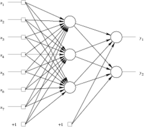
An MLP with a single hidden layer and a linear output layer is essentially a function (7) where W₁ and W₂ are the weight matrices of the hidden and output layer, respectively, b₁ and b₂ are the so-called bias vectors of the same layers and g(·) is the chosen sigmoid function. The function g(·) is not a truly multivariate function, but a simple elementwise one. 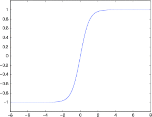For an M-dimensional input vector x = (x₁ x₂ … x_M)^T, it is defined as (8) where g(·) is the actual one-dimensional sigmoid function. In this article, we employ the widely-used hyperbolic tangent function (9) whose behaviour is illustrated in Figure 2.

Figure 2. The hyperbolic tangent function.

The multilayer perceptron is known to be a universal approximator [e.g. 29, which means that for any arbitrary function f(·) and maximum error ϵ that we can tolerate, there exists a number h of hidden neurons with which it is possible to approximate the function f(·) with an error of at most ε. Several studies have been published regarding how to select h [e.g. 30–34 – however, in practice we can often choose a value that is small enough to keep the computation tractable, while being large enough to let us attain an error level that is reasonably low. Typically, there can be a broad range of values enabling approximators that are simply good enough.

Because the hyperbolic tangent function is relatively simple and can easily be implemented using a look-up table, pre-trained MLPs are suitable for online use in many low-cost computing applications.

3.2. Training algorithm

The fact that any function can be approximated by an MLP that is big enough does not mean that it is in practice possible to find the corresponding parameters – i.e. the weight matrices W_i, and the bias vectors b_i. Indeed, there exists a wealth of training algorithms whose purpose is to find such parameters that minimize the chosen cost function. An example of such a cost function is the mean square error (10) where N is the total number of training samples available, M is the dimension of the output vector y, is the kth component of the desired output vector for the jth training sample and is the corresponding element that is output for the same sample by an MLP using the parameters {W_i} and {b_i}.

Most of the existing training algorithms are somehow based on the backpropagation rule presented by Rumelhart et al. in their classic paper 35. In error backpropagation, the gradient of the cost function is calculated with respect to the parameters. This is done first for parameters {W_L} and {b_L} of the output layer, and then subsequently to the earlier layers. The current value of each parameter is moved to the direction of the negative gradient, which is expected to cause a decrease in the value of the cost function. This can be repeated for a predefined number of iterations, or as long as reasonable improvement in the output of the cost function can be observed. In early stopping [e.g. 36, which is a form of regularization, the cost function is evaluated using a separate validation set.

How exactly the updates to the parameter values are made varies between the different algorithms. In this article, we employ the Levenberg–Marquardt algorithm 37.1

When the number of electrodes grows, the number of input variables (voltage measurements related to the different injection patterns) increases rapidly, which slows down the training process. However, many of these input variables correlate strongly between each other. By using principal component analysis [e.g. 39, we can find a linear mapping to a lower-dimensional subspace while preserving as much of the variance in the data as possible. From the practical viewpoint, we found this approach very useful in keeping the computation tractable, even though such a preprocessing step surely results in losing some of the information present in the data.

Moreover, we decided to reduce the variance of the process by actually training an ensemble (or committee) of several networks that vary in complexity (i.e. in the number of hidden neurons). It is well-known [e.g. 40 that such an approach tends to increase the generalization capability (i.e. real-world accuracy) of the eventual estimator.

Note that the training of an MLP (and consequently, that of the ensemble too) typically requires more computing resources by orders of magnitude, when compared to using it in feed-forward mode once the parameters have been fixed.

4. Input variable selection

In this section, we discuss different methods that have been proposed for the selection of input variables. In our case, the input variables to the neural networks being trained are the voltages measured on the different electrodes. Therefore, if we are able to prune some of the input variables without losing a lot of accuracy, it means that we can simply drop the corresponding electrodes from the measurement device (as long as we did not use them for current injection). This makes the device simpler and cheaper to build and maintain.

Variable selection is the art of devising methods that are able to pick only those inputs – i.e. components of x in (7) and (8) – that are relevant for the task at hand. In general, the objective is three-fold 41:

1.	improving the accuracy,
2.	providing faster and more cost-effective analysis, and
3.	understanding what aspects of the underlying process are truly relevant for getting good results.

In the case of EIT for bed level estimation, shrinking the search space might indeed result in regularization that could possibly help improve the accuracy. Moreover, reducing costs is an objective that is highly interesting for us, as already stated earlier in this article. Additionally, we would of course welcome any extra insight into the problem being solved.

Many of the methods for variable selection in machine learning are rooted in the pattern recognition community where the task is often referred to as feature selection and the ultimate goal is the correct classification of data samples. Therefore, not all of the methods are directly useful for regression tasks. In this article, we obviously seek methods that are suitable for bed level measurement in an EIT setting, when using neural networks to learn the mapping from the measured voltage values to (the parameters of) the underlying conductivity distribution.

4.1. From variable selection to electrode selection

Our primary goal is to reduce the number of electrodes, not really the number of input variables (voltage measurements). If we simply pruned the least useful voltage measurements, we would not necessarily be able to drop that many electrodes, as the remaining measurements might be scattered over most of the candidate electrodes. Therefore, we rather consider pruning electrodes directly: the inclusion or exclusion of a single electrode actually implies including or excluding a whole group of voltage measurements, i.e. input variables. What input variables this group comprises is dictated by which other electrodes remain selected.

Therefore, we modify the standard input variable selection algorithms not to select subsets of input variables, but rather subsets of electrodes. Then, for each subset of electrodes being considered, we generate the corresponding measurement pattern, and based on that, the subset of input variables to be assessed. Because the number of candidate electrodes is much smaller than the corresponding number of voltage measurements, this modification makes the search space significantly smaller. An approach like this has previously been called sensor selection (or feature group selection) 42 in order to point out the difference from plain selection of individual input variables.

4.2. Ranking individual variables versus evaluating subsets

The simplest approach to variable selection is the ranking of each individual variable. Algorithms that include doing so either as a preprocessing step or even as their primary means are simple, scalable and have demonstrated empirical success 41. In our case however, it is quite obvious that any electrode alone is not too informative. Moreover, the relevance of any electrode is highly dependent on what other electrodes are available. Therefore, we do not discuss methods that are designed for ranking individual variables.

On the contrary, in subset-based variable selection, the basic idea is that you consider different subsets of all the candidate variables. In order to perform any selection, you first need to be able to somehow evaluate the different subsets. Then, using some search algorithm, you look for subsets that perform well, given the evaluation criterion. We first review in Section 4.3 different ways to evaluate the subsets, and then discuss some relevant search algorithms in Section 4.4.

4.3. Evaluating subsets

In order to be able to select the more useful one, we need to have means of comparing two subsets. The subset assessment methods can basically be divided into two categories:2

1.	In the wrapper approach [e.g. 50, the actual learner is employed as a kind of black box, and its outputs are externally assessed, typically using independent test data.
2.	On the contrary, methods in the filter category [e.g. 51 use means that are independent of the eventual learning algorithm.

If one chooses to use filters, it is typically because they can usually run faster: in the context of hundreds or thousands of input variables, subset evaluation using a wrapper may take a prohibitively long time. However, as the wrapper approach is generally seen to give more accurate results [e.g. 52–54, and we do not intend to try hundreds of different positions for the electrodes, in the context of this article we decided to limit ourselves to the wrapper methodology.

Given a subset, assessment of its capabilities (in the wrapper framework) consists of training an MLP or other learner, and then evaluating its accuracy. In our setting, the simplest way of getting a performance measure is to use the final value of the cost function (10) directly from the training procedure. However, using this training error or apparent error for making further decisions is very rarely a good idea, as it tends to be a highly optimistic estimate. This is because of the fact that if the network has too many hidden neurons, it can easily overfit to the data: for instance, it learns even the noise in the training samples. Also, the more electrodes (and consequently, more input variables) you use, the more optimistic this estimate probably is – which implies that it is not a very good fit for us, since we also want to be able to compare subsets of different sizes to each other in order to make a decision on what subset size is best for our purposes.

In order to get more useful estimates, we can leave part of the data aside during the learning. Once a network has been trained, we feed it with these samples, and then compare the outputs to the known ground-truth values. Essentially, we use (10) such that j iterates only over samples that were not available during the training. The estimate we get this way is called the holdout error. The process can be repeated several times (starting from the split to training and test data), thus averaging out the effects due to a particular, possibly unfortunate division of the data. If this is done in a specific structured manner, then we may be doing cross-validation 55.

4.4. Search for good subsets

A simple approach to finding the best subset is to evaluate all the candidates. This is called exhaustive search: with M candidate electrodes, there are 2^M − M − 1 subsets to be evaluated (we exclude the empty subset that does not include any electrode, and also all subsets containing a single electrode only). It is easy to see that even a moderate number of candidate electrodes makes it impossible to go through every subset, especially if the evaluation of a single subset is not lightning-fast. Therefore, a large number of search strategies have been presented in the literature [e.g. 56 to efficiently evaluate only a necessary number of subsets much lower than 2^M − M − 1, while still reaching near-optimal levels of performance. For the purposes of this article, we discuss two such methods.

4.4.1. Sequential pruning

The first search algorithm that we consider in this article was introduced as early as in 1963 57. Referred to here as sequential backward selection (SBS), the method starts with the set that consists of all the candidate electrodes. During one step of the algorithm, each electrode that is still left in the set is considered to be pruned. The results due to the exclusion of each electrode are compared to each other using the cost function selected. The step is finished by actually pruning the electrode whose removal yields the best result. In this article, steps are taken and electrodes are pruned until only two electrodes remain.

SBS is summarized in Algorithm 1. In the notation used, S and S′ are arrays of Boolean values representing electrode subsets. The binary value S_j indicates whether the jth electrode is selected in S. For clarity, it is assumed here that the cost function E(·) carries the dataset and any evaluator parameters with it.

Algorithm 1

Sequential backward selection algorithm.

function SBS(n,E) Returns a vector of subsets of different sizes (B)

begin E(·) is the function used to evaluate different subsets

  Start with the full set of all n electrodes

 k ≔ n;

 B ≔ ∅; Initialize the vector of best electrode sets found

 while k > 2 Repeat for as long as there are branches to compare

  R ≔ ∅; Initialize the set of evaluations of different branches

  for each { j | S_j = 1} Repeat for each possible branch

   S′ ≔ S; Copy the electrode set

    Prune the jth electrode

   R(j) ≔ E(S′); Evaluate the branch

  end;

  k ≔ k − 1;

  j ≔ argmin R(·); Find the best branch

  S_j ≔ 0; Take the best branch

  B(k) ≔ S; Store the newly found subset

 end;

 return B;

end;

4.4.2. Floating search

A potential problem with the SBS method is that if some electrode happens to be dropped early, it cannot be added again, no matter how useful we might find it later. To remedy this potential issue, various algorithms introducing some sort of backtracking have been suggested in the literature. Here, we present one of the most widely-used approaches: sequential backward floating selection, or SBFS 58.

SBFS consists of two different and alternating phases. The first phase is just one step of SBS. The second phase consists of performing forward selection: electrodes are added to the current set for as long as the subset thus obtained performs better than the best one of its size found so far. When this is no longer the case, the algorithm switches back to the first phase, and continues to prune the electrodes.

The original version of the algorithm contained a minor bug: after some backtracking, when the algorithm switches back to the first phase, it is possible that it ends up with a subset that does not perform as well as the best previously found subset of the same size. Fortunately, the issue can be fixed by abruptly jumping back to this more promising branch 59. The patched version of SBFS is shown in Algorithm 2; the original procedure can be obtained by simply removing the underlined code.

Algorithm 2

Sequential backward floating selection algorithm; the fix by Somol et al. 59 is pointed out by underlining the lines to be added.

function SBFS(n, E) Returns a vector of subsets of different sizes (B)

begin

  Start with the full set of all n electrodes

 k ≔ n;

 B ≔ ∅; Initialize the vector of best electrode sets found

 while k > 2 Repeat for as long as there are branches to compare

  R ≔ ∅; Initialize the set of evaluations of different branches

  for each { j | S_j = 1} Repeat for each possible branch

   S′ ≔ S;

    Prune the jth electrode

   R(j) ≔ E(S′); Evaluate the branch

  end;

  k ≔ k − 1;

  j ≔ argmin R(·); Find the best branch

  if R(j) ≥ E(B(k)) Was this branch the best of its size found so far?

   S ≔ B(k); If no, abruptly switch to the best one

  else

   S_j ≔ 0; If yes, take the branch

   B(k) ≔ S; Store the newly found subset

   t ≔ 1; This is reset when backtracking is to be stopped

   while k < n − 1 ∧ t = 1 Backtrack until no better subsets are found

    R ≔ ∅; Initialize the set of evaluations of different branches

    for each { j | S_j = 0} Repeat for each possible branch

     S′ ≔ S;

      Add the jth electrode

     R(j) ≔ E(S′); Evaluate the branch

    end;

    j ≔ argmin R(·); Find the best branch

    if R(j) < E(B(k + 1)) Was a better subset of size k + 1 found?

     k ≔ k + 1; If yes, backtrack

     S_j ≔ 1;

     B(k) ≔ S; Store the newly found subset

    else

     t ≔ 0; If no, stop backtracking

    end;

   end;

  end;

 end;

 return B;

end;

SBFS obviously evaluates more subsets than SBS does; consequently, running SBFS takes more time. However, in general floating methods have been found 58,60,61 to give results superior to those due to the non-backtracking algorithms – but questions have been asked as well 62. We figured that it is better to try both approaches, and see which one works best for the problem at hand.

5. Simulations

In this section, we describe the experiments that we have conducted. We visualize the results obtained by using the machine learning approach. We discuss the feasibility of estimating the different parameters, including contact impedance. Further, results are presented suggesting that automatic electrode selection can be used to significantly simplify the structure of the probe without making the ultimate measurement results any less accurate.

5.1. Generating the training data

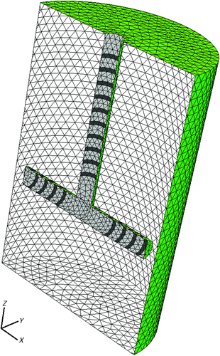
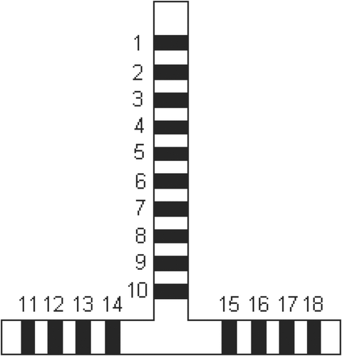
In order to be able to use the machine learning approach described in Section 3, a set of input–output pairs need to be created for training the MLPs. This is done by randomly drawing a number of realistic conductivity distributions and computing the corresponding electrode voltages (i.e. solving the forward problem). In doing this we use a cylindrical domain containing a T-shape probe placed inside. The probe consists of 18 equally-spaced electrodes. The geometry of the domain and the probe is shown in Figure 3.

Figure 3. The measurement geometry for the simulations. Lines in dark gray mark the electrodes.

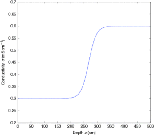
For the FEM computations the domain was discretized using NETGEN 63; the tetrahedral mesh comprised 11,355 nodes. The target was assumed to contain a single bed level only. We also assumed the conductivity distribution of the domain containing the bed level to vary smoothly, and only in the direction of the z axis. Such a situation was modelled using the sigmoid function (11) where σ(z) is the conductivity at depth z, σ₀ and σ₁ the upper and lower conductivities, respectively, D the conductivity transition depth, T the conductivity transition width and a a parameter describing the shape of the sigmoid curve.3 An example of such a transition curve is shown in Figure 4.

Figure 4. A transition curve when σ₀ = 0.3 mS cm⁻¹, σ₁ = 0.6 mS cm⁻¹, D = 250 cm, T = 100 cm and a = 7.

A total of 10,000 values for σ₀, σ₁, T and D were drawn from a uniform random distribution with specified intervals. In addition to this, randomly selected contact impedances z_ℓ were generated.

The current injections were chosen so that currents are propagated all over the whole measurement volume. This kind of a current pattern consists of injections between electrodes that are far away from each other, but also of injections between adjacent electrodes.4 The measurements related to each current injection were performed between the ground electrode of the injection and each other electrode. After generating these kinds of current injection and voltage measurement patterns, the resulting voltages were obtained by solving the forward problem given in Section 2.1. Finally, Gaussian noise with standard deviation of 1% of the corresponding voltage value was added to each measurement.

5.2. Bed level estimation

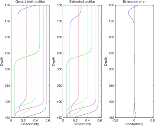
By generating a large number of conductivity profiles and solving the forward problem (Section 2.1) in order to obtain the corresponding simulated voltage measurements, we can come up with a training set for a multilayer perceptron (Section 3.1). In the experiments discussed here, a dataset consisting of 10,000 conductivity profiles was generated. Out of these, 4000 were used to build a training set, 3000 comprised a validation set for early stopping and the remaining 3000 were reserved for final testing. Instead of the raw voltage measurement data, we used the first 32 principal components. An ensemble was put together by training 15 multilayer perceptrons, and selecting those seven (7) that perform best in the sense of the validation error.5 Results on the independent test data are visualized in Figure 5.

Figure 5. Simulated and estimated conductivity profiles using an ensemble of multilayer perceptrons.

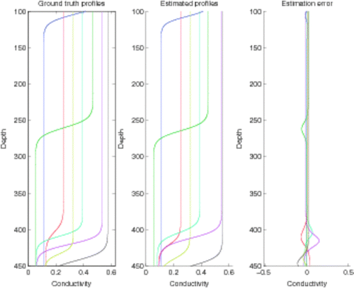
More specifically, each member of the ensemble was trained with the parameters of the corresponding sigmoid function (σ₀, σ₁, D, T) as target outputs,6 and the first 32 principal components of the simulated voltage measurements as the inputs. For the previously unseen test samples, the principal components (as obtained using the transformation matrix due to the training set) of the voltage measurements were fed forward through the perceptrons. Doing so outputs the estimates for the corresponding parameters. Then, based on the estimates for the four parameters, the corresponding profile can be constructed. Therefore, the profiles generated by this approach always correspond to smooth sigmoid functions.

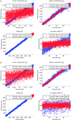
Whereas Figure 5 plots only seven profiles, in Figure 6 we display the correlation between the desired value and the value output by the ensemble for thousands of profiles. Here, we can observe that the transition width T is difficult to estimate, as is the lower conductivity σ₁ whenever the transition takes place below the bottom of the probe. However, the transition depth D, which is the parameter we are most interested in, can be estimated reliably.

Figure 6. The correlation between the ground-truth parameters, and those estimated by the ensemble.

5.3. Contact impedance estimation

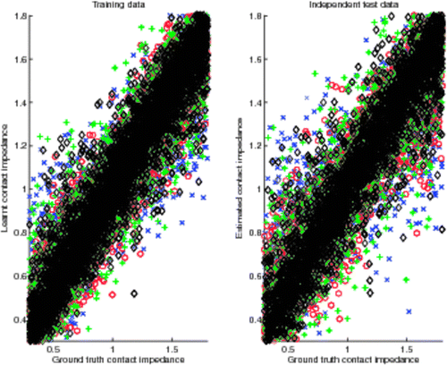
In order to detect a situation where some electrode is building up dirt, the neural networks of an ensemble can be trained to estimate contact impedance (Section 2.1) at each electrode. This is feasible because in addition to the sigmoid parameters (σ₀, σ₁, D, T), the generated contact impedance values are known for every electrode and each simulated profile, and can therefore be used as target output values when training the neural networks. Based on Figure 7, the values are indeed learnt well enough that indicative estimates of dirt build-up can be obtained.

Figure 7. Correlation between ground-truth and estimated contact impedance.

5.4. Selection of electrodes

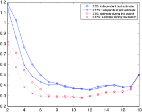
By executing the sequential backward selection (SBS) algorithm described in Section 4.4.1, we get fitness estimates for each electrode subset size from 2 to 18.7 The corresponding criterion curve 61 for independent test data is visualized by the uppermost line of Figure 8. In Section 4, we mentioned that regularization resulting from input variable selection might end up improving accuracy – now, we can see that the removal of one electrode actually helps in decreasing the error estimate. Also, the overfitting of the estimates used to guide the search is evident, when compared to the estimates due to using fresh data that was not available during the search.

Figure 8. Estimation error as the function of the number of electrodes employed.

Based on the uppermost line of Figure 8, we could (somewhat arbitrarily) decide to select six (6) electrodes out of the full set of 18 to be used in the eventual measurement device. By using the best-performing subset of six electrodes, we can repeat the experiment of Section 5.2, and arrive at results like those depicted in Figure 9.

Figure 9. As Figure 5, but using the best subset of 6 electrodes (obtained using the SBS algorithm).

The best-performing subset of six obtained by using the SBS algorithm comprises electrodes 5, 6, 13, 15, 17 and 18. Based on Figure 10 where the positions of the electrodes on the probe are schematically visualized, this kind of non-symmetric selection might seem a bit surprising. However, the injection pattern employed (Section 5.1) was not fully symmetric; and even if it had been, the result would still not imply that some other subsets of the same size could not perform equally well, or even better.

The first one to be pruned was electrode number 10. As its removal improved even the independent test estimate, it seems that there is something misleading in the measurements due to it.

However, the best subset of six electrodes selected by the SBFS algorithm (Section 4.4.2) is composed of electrodes 5, 6, 10, 11, 12 and 18. Based on Figure 8, this subset enables us to obtain better estimates on independent test data, when compared to the subset selected by SBS. Like SBS, also the SBFS algorithm prunes electrode number 10 first, but thanks to its ability to revert this decision later (which is the specific improvement that SBFS has over SBS), it can be put back when it gets useful – i.e. when many of the other electrodes have already been removed from the set.

5.5. Computational complexity

Training in machine learning takes time. Executing a wrapper-based algorithm for input variable selection takes even more time. However, reporting exact computation times would be misleading, because they depend on a number of implementation-specific issues.

Nevertheless, we want to state that in our case, training a single MLP consumed CPU time in the order of minutes when using all the electrodes. As a result, training ensembles took tens of minutes. Moreover, executing SBS kept the processor busy for days. Finally, running the SBFS algorithm – whose worst-case complexity as a function of the number of electrodes is hardly bounded at all – made us wait for weeks. However, it would surely be possible to drastically decrease these run times by optimizing the code and running the experiments on more recent and more powerful hardware.

6. Conclusions

We have described the bed level measurement problem and how to approach it from the electrical impedance tomography point of view. We pointed out the computational complexity of actually solving the inverse problem, and then suggested a way to employ machine learning methodology not only to simplify the computations necessary for online measurements, but also to reduce the dimensionality of the problem, which directly implies a possibility to build considerably cheaper measurement devices.

As we have reported the feasibility of the approach only through simulation studies, our future work should involve experiments in the laboratory, and also in actual process environments.

Figure 10. The electrode numbering of the conductivity probe.

Notes

Notes

1. We first tried with resilient backpropagation 38, but the results were not that good.

2. In addition to these two categories, there is also the embedded approach, in which the selection of variables is part of the training process itself; that idea does not really fit into our division to subset evaluation and subset search. However, embedded methods tend to be highly specific to the learning algorithm. While we do limit ourselves to MLPs in this article – and embedded methods for them surely exist [e.g. 43–49 – it would not be a trivial task to modify these methods to select electrodes rather than individual input variables.

3. It should be noted that various other choices exist to parameterize the conductivity distribution. The chosen model however directly relates to the actual parameters of interest, such as the transition depth.

4. Using the electrode numbering of Figure 10, currents were injected for example between electrodes 1 and 10 and between electrodes 11 and 18, and also between electrodes 9 and 10 and between electrodes 11 and 12.

5. The numbers here were chosen rather arbitrarily; one could call them educated guesses. However, we have no reason to believe that the outcome of using any other reasonable selections would have been significantly worse or better.

6. Note that the output comprises just four parameters, which are then used to generate the actual distribution for the different values of z. As mentioned in Section 3, this is an effective way to regularize the eventual solution.

7. No subset of just one electrode could possibly be useful.

References

- Thelen, TV, Mairal, AP, Thorsen, CS, and Ramirez, WF, 1997. Application of ultrasonic backscattering for level measurement and process monitoring of expanded-bed adsorption columns, Biotechnol. Prog. 13 (5) (1997), pp. 681–687.
- Hjertaker, BT, Johansen, GA, and Jackson, P, 2001. Level measurement and control strategies for subsea separators, J. Electron. Imaging 10 (3) (2001), pp. 679–689.
- Hauptmann, P, Hoppe, N, and Puttmer, A, 2002. Application of ultrasonic sensors in the process industry, Measurement Sci. Technol. 13 (8) (2002), pp. R73–R83.
- Maldonado, M, Desbiens, A, and del Villar, R, 2008. An update on the estimation of the froth depth using conductivity measurements, Minerals Eng. 21 (12) (2008), pp. 856–860.
- Davis, JL, and Annan, AP, 1988. Ground-penetrating radar for high-resolution mapping of soil and rock stratigraphy, Geophys. Prospect. 37 (1988), pp. 531–551.
- M.B. Bashforth and S. Koppenjan, Ground penetrating radar applications for hazardous waste detection, in Proceedings of SPIE, Underground and Obscured-Object Imaging and Detection, Vol. 1942, Orlando, FL, USA, 1993, pp. 56--64.
- Benson, RC, Glaccum, RA, and Noel, MR, 1984. Geophysical Techniques for Sensing Buried Wastes and Waste Migration, Environmental Monitoring Systems Laboratory. Las Vegas: Office of Research and Development, US Environmental Protection Agency; 1984.
- A. Uribe-Salas, M. Leroux, C.O. Gomez, J.A. Finch, and B.J. Huls, A conductivity technique for level detection in flotation cells, in Proceedings of an International Conference on Column Flotation, Vol. II, Sudbury, Ontario, Canada, 1991, pp. 467--478.
- Yang, WQ, Wang, HX, Xie, CG, Brant, MR, and Beck, MS, 1993. "Design and Fabrication of Segmented Capacitance Level Sensor for an Oil Separation Tank". In: in Sensors VI: Technology, Systems and Applications, Proceedings of the Sixth Conference on Sensors and their Applications held 12--15 September 1993 in Manchester (Sensors Series). London: Taylor and Francis; 1993. pp. 369–374.
- Warsito, W, and Fan, L-S, 2003. ECT imaging of three-phase fluidized bed based on three-phase capacitance model, Chem. Eng. Sci. 58 (3--6) (2003), pp. 823–832.
- Bukhari, SFA, and Yang, W, 2006. Multi-interface level sensors and new development in monitoring and control of oil separators, Sensors 6 (2006), pp. 380–389.
- Yang, CN, Chen, SP, and Yang, GG, 2001. Fiber optical liquid level sensor under cryogenic environment, Sensors and Actuators A: Physical 94 (1) (2001), pp. 69–75.
- Chakravarthy, S, Sharma, R, and Kasturi, R, 2002. Noncontact level sensing technique using computer vision, IEEE Trans. Instrument. Measurement 51 (2) (2002), pp. 353–361.
- Golnabi, H, 2004. Design and operation of a fibre optic sensor for liquid level detection, Optics Lasers Eng. 41 (5) (2004), pp. 801–812.
- Adler, A, and Guardo, R, 1994. A neural network image reconstruction technique for electrical impedance tomography, IEEE Trans. Med. Imaging 13 (4) (1994), pp. 594–600.
- Nooralahiyan, AY, and Hoyle, BS, 1997. Three-component tomographic flow imaging using artificial neural network reconstruction, Chem. Eng. Sci. 52 (13) (1997), pp. 2139–2148.
- Nejatali, A, and Ciric, IR, 1998. An iterative algorithm for electrical impedance imaging using neural networks, IEEE Trans. Magnetics 34 (5) (1998), pp. 2940–2943.
- Ratajewicz-Mikolajczak, E, Shirkoohi, GH, and Sikora, J, 1998. Two ANN reconstruction methods for electrical impedance tomography, IEEE Trans. Magnetics 34 (5) (1998), pp. 2964–2967.
- J. Lampinen, A. Vehtari, and K. Leinonen, Using Bayesian neural network to solve the inverse problem in electrical impedance tomography, in Proceedings of the 11th Scandinavian Conference on Image Analysis (SCIA'99), Vol. 1, 1999, pp. 87--93.
- Teague, G, Tapson, J, and Smit, Q, 2001. Neural network reconstruction for tomography of a gravel–air–seawater mixture, Measurement Sci. Technol. 12 (2001), pp. 1102–1108.
- Kaipio, JP, and Somersalo, E, 2004. Statistical and Computational Inverse Problems, Applied Mathematical Sciences. Vol. 160. New York: Springer; 2004.
- Cheng, K-S, Isaacson, D, Newell, J, and Gisser, D, 1989. Electrode models for electric current computed tomography, IEEE Trans. Biomed. Eng. 36 (1989), pp. 918–924.
- Somersalo, E, Cheney, M, and Isaacson, D, 1992. Existence and uniqueness for electrode models for electric current computed tomograpgy, SIAM J. Appl. Math. 52 (1992), pp. 1023–1040.
- Vauhkonen, M, Vadász, D, Karjalainen, P, Somersalo, E, and Kaipio, J, 1998. Tikhonov regularization and prior information in electrical impedance tomography, IEEE Trans. Biomed. Eng. 45 (1998), pp. 486–493.
- M. Vauhkonen, Electrical Impedance Tomography and Prior Information, PhD thesis, University of Kuopio, Kuopio, Finland, 1997.
- Vauhkonen, PJ, Vauhkonen, M, Savolainen, T, and Kaipio, JP, 1999. Three-dimensional electrical impedance tomography based on the complete electrode model, IEEE Trans. Biomed. Eng. 46 (9) (1999), pp. 1150–1160.
- Cheney, M, Isaacson, D, and Newell, JC, 1999. Electrical impedance tomography, SIAM Rev. 41 (1) (1999), pp. 85–101.
- Rosenblatt, F, 1958. The perceptron: A probabilistic model for information storage and organization in the brain, Psychol. Rev. 65 (6) (1958), pp. 386–408.
- Tikk, D, Kóczy, LT, and Gedeon, TD, 2003. A survey on universal approximation and its limits in soft computing techniques, Int. J. Approx. Reason. 33 (2) (2003), pp. 185–202.
- S.Y. Kung and J.N. Hwang, An algebraic projection analysis for optimal hidden units size and learning rates in back-propagation learning, in Proceedings of the IEEE International Conference on Neural Networks, San Diego, CA, USA, 1988, pp. 363--370.
- Huang, S-C, and Huang, Y-F, 1991. Bounds on the number of hidden neurons in multilayer perceptrons, IEEE Trans. Neural Networks 2 (1) (1991), pp. 47–55.
- Murata, N, Yoshizawa, S, and Amari, S, 1994. Network information criterion – determining the number of hidden units for an artificial neural network model, IEEE Trans. Neural Networks 5 (6) (1994), pp. 865–872.
- Camargo, LS, and Yoneyama, T, 2001. Specification of training sets and the number of hidden neurons for multilayer perceptrons, Neural Comput. 13 (12) (2001), pp. 2673–2680.
- Teoh, EJ, Tan, KC, and Xiang, C, 2006. Estimating the number of hidden neurons in a feedforward network using the singular value decomposition, IEEE Trans. Neural Networks 17 (6) (2006), pp. 1623–1629.
- Rumelhart, DE, Hinton, GE, and Williams, RJ, 1986. "Learning internal representations by error propagation". In: Rumelhart, D.E., McClelland, J.L., and the PDP Research Group, , eds. Parallel Distributed Processing: Explorations in the Microstructure of Cognition. Volume 1: Foundations. Cambridge, MA: MIT Press; 1986. pp. 318–362.
- W.S. Sarle, Stopped training and other remedies for overfitting, in Proceedings of the 27th Symposium on the Interface of Computing Science and Statistics, Pittsburgh, PA, USA, 1995, pp. 352--360.
- Hagan, MT, and Menhaj, MB, 1994. Training feedforward networks with the Marquardt algorithm, IEEE Trans. Neural Networks 5 (6) (1994), pp. 989–993.
- M. Riedmiller and H. Braun, A direct adaptive method for faster backpropagation learning: The RPROP algorithm, in Proceedings of the IEEE International Conference on Neural Networks, San Francisco, CA, USA, 1993, pp. 586--591.
- Jolliffe, IT, 2002. Principal Component Analysis, . New York: Springer; 2002.
- Dietterich, TG, 2000. "Ensemble methods in machine learning". In: Kittler, J., and Roli, F., eds. Multiple Classifier Systems, Vol. 1857 of LNCS. Berlin, Heidelberg: Springer; 2000. pp. 1–15.
- Guyon, I, and Elisseeff, A, 2003. An introduction to variable and feature selection, J. Machine Learn. Res. 3 (2003), pp. 1157–1182.
- Subrahmanya, N, and Shin, YC, 2008. Automated sensor selection and fusion for monitoring and diagnostics of plunge grinding, J. Manufactur. Sci. Eng. 130 (3) (2008), pp. 1–11, 031014.
- Le Cun, Y, Denker, JS, and Solla, SA, 1990. "Optimal brain damage". In: Touretzky, D.S., ed. Advances in Neural Information Processing Systems II. San Francisco: Morgan Kaufmann; 1990. pp. 598–605.
- Hassibi, B, and Stork, DG, 1993. "Second order derivatives for network pruning: Optimal brain surgeon". In: Hanson, S.J., Cowan, J.D., and Giles, C.L., eds. Advances in Neural Information Processing Systems 5. San Mateo, CA: Morgan Kaufmann; 1993. pp. 164–171.
- T. Cibas, F. Soulié, P. Gallinari, and S. Raudys, Variable selection with optimal cell damage, in Proceedings of the 4th International Conference on Artificial Neural Networks (ICANN'94), Sorrento, Italy, 1994, pp. 727--730.
- Cibas, T, Soulié, F, Gallinari, P, and Raudys, S, 1996. Variable selection with neural networks, Neurocomputing 12 (2--3) (1996), pp. 223–248.
- De, RK, Pal, NR, and Pal, SK, 1997. Feature analysis: Neural network and fuzzy set theoretic approaches, Pattern Recognition 30 (10) (1997), pp. 1579–1590.
- Setiono, R, and Liu, H, 1997. Neural-network feature selector, IEEE Trans. Neural Networks 8 (3) (1997), pp. 654–662.
- Egmont-Petersen, M, Talmon, JL, Hasman, A, and Ambergen, AW, 1998. Assessing the importance of features for multi-layer perceptrons, Neural Networks 11 (4) (1998), pp. 623–635.
- Kohavi, R, and John, G, 1997. Wrappers for feature subset selection, Artificial Intelligence 97 (1--2) (1997), pp. 273–324.
- Duch, W, 2006. "Filter methods". In: Guyon, I., Gunn, S., Nikravesh, M., and Zadeh, L.A., eds. Feature Extraction – Foundations and Applications. Berlin, Heidelberg: Springer; 2006. pp. 89–117.
- Aha, DW, and Bankert, RL, 1996. "A comparative evaluation of sequential feature selection algorithms". In: Fisher, D.H., and Lenz, H.-J., eds. Learning from Data: Artificial Intelligence and Statistics V. New York: Springer-Verlag; 1996. pp. 199–206.
- Inza, I, Larrañaga, P, Blanco, R, and Cerrolaza, AJ, 2004. Filter versus wrapper gene selection approaches in DNA microarray domains, Artificial Intelligence Med. 31 (2) (2004), pp. 91–103.
- Somol, P, Baesens, B, Pudil, P, and Vanthienen, J, 2005. Filter- versus wrapper-based feature selection for credit scoring, Int. J. Intelligent Syst. 20 (10) (2005), pp. 985–999.
- Stone, M, 1974. Cross-validatory choice and assessment of statistical predictions, J. Roy. Stat. Soc. 36 (2) (1974), pp. 111–133.
- Reunanen, J, 2006. "Search strategies". In: Guyon, I., Gunn, S., Nikravesh, M., and Zadeh, L.A., eds. Feature Extraction – Foundations and Applications. Berlin, Heidelberg: Springer; 2006. pp. 119–136.
- Marill, T, and Green, DM, 1963. On the effectiveness of receptors in recognition systems, IEEE Trans. Information Theory 9 (1) (1963), pp. 11–17.
- Pudil, P, Novovičová, J, and Kittler, J, 1994. Floating search methods in feature selection, Pattern Recognition Lett. 15 (11) (1994), pp. 1119–1125.
- Somol, P, Pudil, P, Novovičová, J, and Paclík, P, 1999. Adaptive floating search methods in feature selection, Pattern Recognition Lett. 20 (11--13) (1999), pp. 1157–1163.
- Jain, AK, and Zongker, D, 1997. Feature selection: Evaluation, application, and small sample performance, IEEE Trans. Pattern Anal. Machine Intelligence 19 (2) (1997), pp. 153–158.
- Kudo, M, and Sklansky, J, 2000. Comparison of algorithms that select features for pattern classifiers, Pattern Recognition 33 (1) (2000), pp. 25–41.
- Reunanen, J, 2003. Overfitting in making comparisons between variable selection methods, J. Machine Learn. Res. 3 (2003), pp. 1371–1382.
- Netgen – automatic mesh generator. Software available at http://www.hpfem.jku.at/netgen/.