Reconstruction of moving boundary for one-dimensional heat conduction equation by using the Lie-group shooting method

Abstract

We consider an inverse problem for the recovery of an unknown time-dependent moving boundary ξ(t) in a one-dimensional heat conduction equation. By using the domain embedding technique, the inverse problem of moving boundary identification is transformed into a time-dependent parameter function identification problem of an advection–diffusion partial differential equation, where ξ(t) and play the role of unknown parameters. From a viewpoint of numerical differentiation, that appearing in the governing equation causes the identification of ξ(t) being rather difficult, because the differential itself is an ill-posed operator. In order to overcome this difficulty we let , instead of ξ(t), be the unknown variable, and ξ(t) is calculated from by an integration. Once using the Lie-group shooting method (LGSM) we can derive a quite simple system of linear algebraic equations to iteratively calculate and then ξ(t). It is demonstrated through numerical examples that the LGSM is accurate, efficient and stable; the maximum error of numerical solutions is in the order of 10⁻⁴–10⁻², even a large noise in the level of 10⁻² is imposed on the measured data.

Keywords:

• inverse problem
• moving boundary identification
• Lie-group shooting method
• Time-dependent moving boundary

1. Introduction

The free boundary problems for heat conduction equation are those in which the unknown spatial domain varies with time, and the law of the movement of the boundary is not yet known. In order to determine the moving boundary, we need to impose another condition on the unknown function, which will depend on the physical problems we study. For example, for the monitoring of iron manufacturing blast furance 1, we can simultaneously measure the temperature and heat flux on an accessible part of boundary, and then use the inversion technique to determine the moving boundary.

Applications of inverse boundary determination problems span over many heat transfer related topics. Among those problems we may have the inverse Stefan problem, diffusion-consumption of oxygen in a living tissue, continuous casting problem and other solidification processes. Evans and King 2 have given a description of the models on how they led to the one-dimensional moving boundary problem. Sometimes the temperature and heat flux data on the accessible part of a boundary are known and one wants to determine the movement of unknown boundary. Those problems are often referred to as the boundary identification problems in the literature 3. Most inverse problems of the boundary identification belong to a family of problems that have inherited the property of being ill-posed in the sense of Hadamard 4.

Banks and Kojima 5 and Banks et al. 6 have proposed some reconstruction methods for the boundary determination problems of parabolic equations. Such a problem has been studied by using the traditional optimization-based fit-to-data approaches, or by converting the inverse problem into a version of the so-called sideways heat equation 1. The situation is somewhat like as the coefficient recovery problems for parabolic equations 7.

This study estimates the time-varying moving boundary by solving an inverse heat conduction problem under an overspecified boundary data. The estimation is based on a transient temperature gradient measurement undertaken by inserting two near thermocouples adjacent to a fixed boundary of a heat conducting body. Our approach of this difficult inverse problem is adopting the numerical method of lines together with the group preserving scheme (GPS) developed previously by Liu 8 for ordinary differential equations (ODEs). Recently, Liu 9–11 has extended the technique of GPS to solve the boundary value problems (BVPs), and the numerical results revealed that the GPS is a rather promising method to effectively solve the two-point BVPs. In the construction of the Lie-group method for the computations of BVPs, Liu 9 has introduced the idea of one-step GPS by utilizing the closure property of the Lie group, and hence, the new shooting method has been named the LGSM. The LGSM is also shown effective to the second-order general BVPs 10, the singularly perturbed BVPs 11, the Sturm–Liouville eigenvalue problems 12, as well as the generalized Sturm–Liouville problems 13.

In a series of papers by the author and his coworkers, the Lie-group method exhibited its excellent behaviour on the numerical solutions of BVPs and inverse problems. Liu 14–16 has used the concept of one-step GPS to develop the numerical method for the estimation of unknown temperature-dependent heat conductivity and heat capacity, Chang et al. 17 to treat the sideways heat conduction problems, Chang et al. 18 to treat the boundary layer equation in fluid mechanics, and Liu 19, Liu et al. 20, and Chang et al. 21 to treat the backward heat conduction equation and Liu et al. 22 to treat the Burgers equation.

By taking the advantage of the Lie-group method, Liu 23 could accurately solve the inverse heat conduction problems of identifying the non-homogeneous heat conductivity functions, in 24 he has solved the inverse Sturm–Liouville problems and in 25 he has solved the inverse vibration problems. Liu 26 has used the idea of Lie-group shooting method to solve the identification problem of time-dependent heat conductivity function, and in 27 he has further developed a two-stage LGSM to identify a time-dependent heat source through a measurement of internal temperature. Then, Liu 28 developed a highly stable LGSM in the spatial direction to identify the initial temperature for the backward heat conduction problem, which allows a large elapsed-time.

It is interesting to note that the LGSM does not require a priori regularization when we apply it to the inverse problem, and also exhibits several advantages than other methods. It would be clear that the new method can greatly reduce the computational time and is very easy to numerical implement to the computations of inverse problem of boundary identification. Especially, the present LGSM can provide a better computational result, and we eagerly suggest that by using the LGSM we can solve these computations of inverse problems for the identification of moving boundary.

As the Lie-group method possesses some certain advantages than other numerical methods due to its Lie-group structure, the LGSM has been shown to be a powerful technique to solve the inverse problems of parameters identification as mentioned above. However, the methodology of LGSM is rarely applied to the identification of parabolic type linear partial differential equation (PDEs) with a time-dependent moving boundary in the open literature. Thus we attempt to develop an effective, accurate and stable numerical method of the LGSM type for this useful inverse problem of moving boundary identification. The novelty presented in this article will be that we transform the identification problem of time-dependent moving boundary into a parameter identification problem of PDE including a rate term of the identified time-dependent parameter, and that we can propose a stable algorithm to recover the moving boundary by resolving the difficulty resulted from the rate term.

2. Formulation of the moving-boundary problem

We consider a one-dimensional heat conduction equation with a moving boundary ξ(t): (1) and the Cauchy data are over-specified at the left-boundary: (2) where u(y, t) is the temperature distribution and t_f > 0 represents an arbitrary final time of interest. The boundary identification problem is then the determination of the boundary movement function ξ(t) from a Dirichlet boundary condition: (3) where u_ξ(t) is a given function, usually being a constant or zero. Let (4) and from Equations (1–3) it follows that (5) (6) (7)

The domain embedding method by transforming the moving boundary into a fixed boundary is widely used to solve the free-boundary problems; see for example, Murray and Landis 29 and Finlayson 30. Liu and Guerrier 31 have used this method together with a regularization technique to solve the inverse Stefan problem. Recently, Slota and Zielonka 32 have employed this technique together with a variational iteration method to solve the inverse Stefan problem. Hon and Li 33 have applied a meshless method of fundamental solutions (MFS) to solve the above problem.

The appearance of in the governing PDE in Equation (5) makes the identification of ξ(t) being quite difficult from a viewpoint of numerical differentiation 34, because the differential itself is an ill-posed operation. A new method will be developed to recover the unknown function ξ(t) of the above inverse problem, which is subjected to the overspecified boundary conditions in Equations (6) and (7). By using the LGSM we can derive a very simple system of linear algebraic equations to iteratively solve and then ξ(t).

The solution of ξ(t) may be non-unique; for example, for we have two solutions: both satisfying u(ξ(t), t) = 0. Wei and Yamamoto 35 have derived the conditions for the uniqueness of ξ(t); refer also Manselli and Vessella 36. Furthermore, Wei and Yamamoto 35 have discussed the numerical method for the same inverse problem without initial data. There are very few papers for the same inverse problem without needing initial data.

3. Mathematical preliminaries

3.1. The numerical procedures

We are going to solve the present inverse problem of boundary identification through two steps. First, we solve the advection–diffusion Equation (5) in the spatial interval of 0 < x < 1 by subjecting it to the initial condition, and the Dirichlet boundary conditions. For this purpose, Equation (5) is transformed into the following equations: (8) (9) Then, by using a semi-discretization method to discretize the quantities of T(x, t) and S(x, t) in the time domain, we can obtain a system of ODEs for T and S with x as an independent variable. Second, the LGSM as first developed by Liu 9 is extended and applied to the following discretized equations: (10) (11) (12) (13) where Δt = t_f/(n − 1) is a uniform time increment, and t_i = (i − 1)Δt are the discretized times. Here, T_i(x) = T(x, t_i), S_i(x) = S(x, t_i) and ξ_i = ξ(t_i) are the discretized quantities at the nodal points of time. While the central difference is used in Equation (12), we may use the forward difference in Equation (11) at the first time point and the backward difference in Equation (13) at the last time point in order to maintain the same second-order accuracy.

The following three boundary conditions are known and given by (14) (15) (16) which are obtained from Equations (6) and (7) by discretizations.

We will develop a numerical method to calculate the coefficients ξ_i and based on the numerical method of lines which leads to a set of ODEs as shown above. In order to explore our new method self-content, let us first briefly sketch the GPS for ODEs and one-step GPS in this section. The readers may refer the author's papers listed in ‘References’ for a detailed treatment.

3.2. The GPS

Lie-group is a differentiable manifold, endowing a group structure that is compatible with the underlying topology of manifold. The main purpose of Lie-group solver is to provide a better algorithm that retains the orbit generated from numerical solution on the manifold which is associated with the Lie-group 37. The retention of Lie-group structure under discretization is vital in the recovery of qualitatively correct behaviour in the minimization of numerical error 38.

Let us write Equations (10–13) in a vector form: (17) where the prime denotes the differential with respect to x, and (18) in which T = (T₁, … , T_n)^t and S = (S₁, … , S_n)^t. The components of h₂ represent the right-hand sides of Equations (11–13).

When both the vector y and its magnitude are combined into a single augmented vector: (19) Liu 8 has transformed Equation (17) into an augmented differential system: (20) where A is an element of the Lie algebra so(2n, 1) satisfying (21) and (22) is a Minkowski metric. Here, I_2n is the identity matrix, and the superscript t stands for the transpose.

The augmented variable X can be viewed as a point in the Minkowski space 𝕄²ⁿ⁺¹, by satisfying a cone condition: (23)

Accordingly, Liu 8 has developed a GPS to guarantee that each X_k can automatically locate on the cone: (24) where X_k denotes the numerical value of X at the discrete x_k, and G(k) ∈ SO_o(2n, 1) satisfies (25) (26) (27) where is the 00-th component of G.

Quite differently, Ying and Candés 39 have introduced a phase flow method for non-linear ODEs in Equation (17) by setting Therefore, the original n-dimensional ODEs system is embedded into an (n + 1)-dimensional system in the space of (u, t). This technique is not at all a new one, which was already appeared in many textbooks of ODEs to treat the non-autonomous ODEs system as an autonomous one. However, Ying and Candés 39 have used this technique to construct a novel and accurate approach for the phase flow maps of certain ODEs. The above augmented system is drastically different from the one in Equation (20). The main features of our formulation in Equation (20) are three-fold: (1) a geometric cone structure, (2) a Lie-algebra structure and then (3) a Lie-group structure of SO_o(2n, 1). Even the phase flow method may have a Lie-group structure, but it is hard to find this Lie-group mapping; more precisely, finding this Lie-group transformation of phase flow is equivalent to finding the mapping on the solution curves of the original non-linear ODEs.

3.3. One-step Lie-group transformation

Throughout this article we use the superscripted symbols y⁰ to denote the value of y at x = 0, and y¹ the value of y at x = 1. Notice that y⁰ cannot be a zero vector, i.e. ‖y⁰‖ > 0; otherwise, from Equation (17) it follows that y ≡ 0 for all x ∈ (0, 1].

Applying scheme (24) to Equation (20) with a specified left-boundary condition X(0) = X⁰ we can compute the solution X(x) by the GPS. Assuming that the spatial stepsize used in the GPS is Δx = 1/K, and starting from an augmented left-boundary condition X⁰ = ((y⁰)^t, ‖y⁰‖)^t ≠ 0 we can calculate the value X¹ = ((y¹)^t, ‖y¹‖)^t at the right-boundary x = 1.

By applying Equation (24) step-by-step we can obtain (28) However, let us recall that each G_i, i = 1, … , K, is an element of the Lie-group SO_o(2n, 1), and by the closure property of the Lie group, G_K(Δx) ··· G₁(Δx) is also a Lie-group element denoted by G. Hence, from Equation (28) it follows that (29) This is a one-step Lie-group transformation from X⁰ to X¹.

It should be stressed that the one-step Lie-group transformation property is usually not shared by other numerical methods, because those methods do not belong to the Lie-group schemes. This important property has first pointed out by Liu 40 and used to solve the backward in time Burgers equation. After that Liu 14 has used this concept to establish a one-step estimation method to estimate the temperature-dependent heat conductivity, and then extended to estimate thermophysical properties of heat conductivity and heat capacity 15,16,41.

The remaining problem is how to construct G. While an exact solution of G is not possible, we can calculate G through a numerical method by a generalized mid-point rule, which is obtained from an exponential mapping of A by taking the values of the argument variables of A at a generalized mid-point. The Lie-group element generated from such an A ∈ so(2n, 1) by an exponential mapping is (30) where (31) (32) (33) Here, we use the left-side y⁰ = (T(0), S(0)) and the right-side y¹ = (T(1), S(1)) through a suitable weighting factor r to calculate G, where and r ∈ [0, 1] is a parameter to be determined by matching the target specified by the given right-side boundary condition. To emphasize its dependence on r we denote this G by G(r), which is a single-parameter Lie-group element.

3.4. A Lie-group shooting equation

Let us define a new vector (34) such that Equations (30) and (33) can be expressed as (35) (36) From Equations (19), (29) and (35) it follows that (37) (38) where (39) Substituting F in Equation (37), which is re-written as (40) into Equation (38) and dividing both the sides by ‖y⁰‖, we can obtain (41) where, after inserting Equation (40) for F into Equation (36), a and b are now written as (42) Let (43) (44) and thus from Equations (41) and (42) it follows that (45)  Upon defining (46) from Equation (45) we can obtain a quadratic equation for Z: (47) On the other hand, by inserting Equation (40) for F into Equation (39) we can obtain (48) Dividing both sides by ‖y⁰‖‖y¹ − y⁰‖ and using Equations (42–44) and (46) we can also obtain another quadratic equation for Z: (49) From Equations (47) and (49), the solution of Z is found to be (50) and by Equations (46) and (44) we have (51)

Up to this point, we have obtained an important result that between any two points (y⁰, ‖y⁰‖) and (y¹, ‖y¹‖) on the cone, there exists a Lie group element G ∈ SO_o(2n, 1), which upon mapping (y⁰, ‖y⁰‖) onto (y¹, ‖y¹‖): (52) where G is uniquely determined by y⁰ and y¹ through the following equations: (53) (54) (55) In view of Equations (43), (50) and (51), it can be seen that G is fully determined by y⁰ and y¹. Therefore we obtain a very important Lie-group shooting equation: (56)

4. The LGSM

From Equations (10–15) it follows that (57) (58) (59) (60) where T⁰, T¹ and S⁰ are known from Equations (14–16).

By using Equation (18) for y we have (61) and further inserting them into Equation (40) yields (62)

From Equations (43), (50) and (51) by inserting Equation (61) for y⁰ and y¹ we can obtain (63) (64) (65) Comparing Equation (62) with Equation (34) and by Equations (18) and (61), one has (66) (67) where (68) (69)

For the use in the later, , , H¹ and H² are written out explicitly: (70) (71) where , , , and ξ_i = ξ(t_i), i = 1, … , n are the discretized values of the continuous time moving boundary ξ(t).

4.1. A linearly moving boundary

In this section we consider that the moving boundary is a linear function of t, i.e. ξ(t) = at + b, where a is an unknown constant, and b is determined by the initial value of ξ(0). For a slowly varying boundary the above formula may be a good approximation.

By Equations (70) and (71) we have (72) (73) and from Equations (67) and (66) it follows that (74) (75)

Taking the ratio of the above two equations leads to (76) Through some manipulations we can obtain a quadratic equation to solve : (77) If the following condition for the discriminant is satisfied: (78) we have a solution: (79) Then from Equation (75) we have a closed-form solution for ξ_i: (80)

When ξ_i is obtained we can obtain the constant a in ξ(t) = at + b by an iteration process. By using the least-squares method to (81) leads to (82) Choose an initial value of a₀, and thus in Equation (71) is available. By Equations (80) and (82) we can calculate the new a. Repeating the process until the solutions of ξ_i and a are convergent.

Because T⁰, T¹, S⁰ are all available as follows: (83) we can use Equations (79) and (80) to calculate the coefficients ξ_i for a specified r under the condition of D ≥ 0. Then, we can return to Equations (10–12) by inserting and ξ_i, and integrating them to obtain T(1) and S(1). The above process can be done for all r in the interval of r ∈ [0, 1] with D ≥ 0. Among these solutions we can pick up the best r, which leads to the smallest error of (84) such that the right-boundary condition specified by Equation (6) can be fulfilled to the best.

4.2. A non-linearly moving boundary

There are two methodologies based on the LGSM to recover the unknown moving boundary.

4.2.1. The first scheme with an inner iteration

For the non-linearly moving boundary identification problem we can suppose that when are unknowns, ξ_i are calculated by the following recurrent formula: (85) The numerical procedures for computing ξ_i and are described as follows. We start by assuming one set of the initial values of , and substituting ξ_i and into Equations (10–12) we can apply the fourth-order Runge-Kutta method (RK4) or the GPS to integrate them from x = 0 to x = 1. Then, we can obtain . Inserting and the exact , and given by Equation (83) into Equation (76), we can calculate the new by (86) where the components of are given by Equation (71). The new are then compared with the old ones. If the difference is smaller than a given criterion, then we stop the iteration process, and the final ξ_i and are obtained. For each given r we can perform the above procedures. Among these solutions of ξ_i and we choose the best one to fit the minimum criterion given in Equation (84).

It can be seen that Equation (86) is a quite simple linear equation to iteratively solve . Indeed, because the iteration processes based on Equations (86) and (85) are quite simple and stable, the convergence is very fast.

4.2.2. The second scheme without an inner iteration

From Equations (74) and (75) we can solve (87) (88) The present procedure is given as follows. For each given r, we start by assuming one set of the initial values of and , calculate ξ_i from Equation (85), and then use the above two equations to produce the new and until they are convergent according to a given convergence criterion. Substituting and ξ_i into Equations (10–12) and using the given initial conditions of and we can apply the GPS to integrate them from x = 0 to x = 1. Then, we can obtain . For each r we can perform the above procedures. Among these solutions of ξ_i, and , we can choose the best one to fit the minimum criterion given in Equation (84).

Although, our starting point for the moving-boundary identification problem is the ODEs in Equations (8) and (9), the final Equation (86) can be used to any other type approximations, which are only required to provide the necessary discretized data on the boundary, such as , , and . Using those data we can adjust the speed of moving boundary by Equation (86). In this sense, the LGSM can be combined together with other numerical methods without difficulty. For example, the missing data in , , and can also be obtained by using the MFS. Therefore, we can have a large scope by combining the LGSM with other methods to well solve the inverse problems. This important issue will be pursued in the near future.

5. Numerical examples

Now, we are ready to apply the LGSM to the solution of ξ(t) through some tests by numerical examples. When the input measured Cauchy data are contaminated by random noise, we take (89) where δ specifies the level of noise, and R(i) are random numbers in [−1, 1].

5.1. Example 1

The exact solution of Equations (1–3) is chosen as (90) The other data can be derived easily, where ξ(t) = 1 − t/2 is a linear function of t and u_ξ(t) = 0.

Before employing the numerical method of LGSM to calculate this example we use it to demonstrate how to pick up the best r as specified by Equation (84). In Figure 1(a) we plot the mismatching to the target with respect to r in a larger range of 0 ≤ r ≤ 0.6. It can be seen that there exists a minimum point at which the mismatching to the target is the smallest. In order to pick up a better r we plot the mismatching to the target with respect to r in a finer range of 0.53 ≤ r ≤ 0.54 in Figure 1(b). Hence, it is not difficult to choose the best r.

Figure 1. For Example 1: (a) and (b) plots of the error of mismatching to the target, and (c) comparison of the numerical solutions with the exact one.

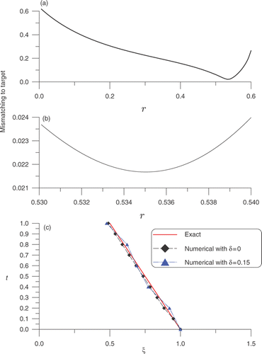
This example has been calculated by Liu and Guerrier 31 and Wei and Yamamoto 35. Our results as shown in Figure 1(c) are rather accurate with the maximum error for δ = 0 with 1.55 × 10⁻² and 2.78 × 10⁻² for δ = 0.15. It shows that the LGSM is very stable against the noise.

5.2. Example 2

The exact solution is chosen as (91) with the moving boundary for u_ξ(t) = 0 given by (92) and other functions are (93)

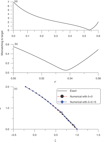
First, we apply the technique in Section 4.1 to find ξ_i with an initial choice of a₀ = − 0.5. In Figure 2(a) we plot the mismatching to the target with respect to r in a larger range of 0 ≤ r ≤ 0.6. It can be seen that there exists a minimum point at which the mismatching to the target is the smallest. In order to pick up a better r we plot the mismatching to the target with respect to r in a finer range of 0.5 ≤ r ≤ 0.56 in Figure 2(b). Then under the parameters Δx = 1/50, Δ t = 0.1 and t_f = 2 used in this computation, we compare the exact solution of ξ(t) with the numerical solutions without considering noise and that with a noise δ = 0.15 in Figure 2(c). For the former case the maximum error is 1.26 × 10⁻², and for the latter case the maximum error is 3.28 × 10⁻². Even under a stringent convergence criterion with ϵ = 10⁻⁸, the finding of a is very fast convergent with only three or four iterations. It can be seen that a large noise with δ = 0.15 only disturbed the numerical solution from the exact one a little.

Figure 2. For Example 2: (a) and (b) plots of the error of mismatching to the target, and (c) comparison of the numerical solutions obtained from Section 4.1 with the exact one.

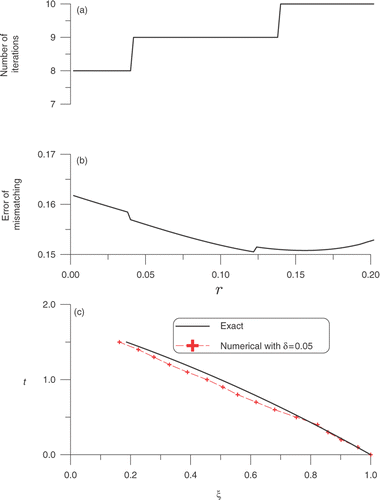
Next, we apply the technique in Section 4.2.1 to solve this problem. For each r in the range of 0 ≤ r ≤ 0.2, we plot the number of iterations with respect to r in Figure 3(a), of which we can see that the convergence is very fast. In Figure 3(b) we plot the mismatching to the target with respect to r in the range of 0 ≤ r ≤ 0.2. Even under a large noise with δ = 0.05, the numerical solution is also close to the exact one as shown in Figure 3(c).

Figure 3. For Example 2: (a) the number of iterations, (b) plot of the error of mismatching to the target, and (c) comparing the numerical solution obtained from Section 4.2.1 with the exact one.

5.3. Example 3

The exact solution of Equations (1–3) is chosen as 33 (94) We apply the technique in Section 4.2.1 to solve this problem with u_ξ(t) = 4.

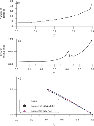
The number of iterations is plotted in Figure 4(a) with respect to r in the range of 0 ≤ r ≤ 0.4 under a convergence criterion ϵ = 10⁻³. In Figure 4(b) we plot the mismatching to the target with respect to r in the range of 0 ≤ r ≤ 0.6. When there exists no noise in the data the present algorithm leads to a rather accurate result with a maximum error 5 × 10⁻³ as shown in Figure 4(c) by the solid line marked by triangles. Even under a noise with δ = 0.01, the numerical solution is also close to the exact one as shown in Figure 4(c) by the dashed line marked by black solid points.

Figure 4. For Example 3: (a) the number of iterations, (b) plot of the error of mismatching to the target, and (c) comparison of the numerical solutions obtained from Section 4.2.1 with the exact one.

5.4. Example 4

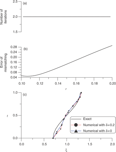
The moving boundary is supposed to be (95) and u_ξ(t) = 0. The Neumann data are q₀(t) = 1 and the Dirichlet data at the left-boundary x = 0 are obtained by solving a direct problem with u(y, 0) = y − 1. We apply the MFS to derive a linear algebraic equations system with the source points and collocation points as shown in Figure 5(a). Then the linear system is post-conditioned by using the Laplacian conditioner introduced by Liu et al. 42 and Liu 43. The datum of u₀(t) is plotted in Figure 5(b). We apply the scheme in Section 4.2.2 to solve this problem. When there exists no noise on the input data we obtain the numerical result with a maximum error 1.26 × 10⁻² as shown in Figure 6(c) by the solid line marked by triangles. In Figure 6(a) we plot the number of iterations with respect to r, which shows that the algorithm given in Section 4.2.2 converges very fast. Under a noise with δ = 0.2, while the mismatching curve in the range of 0.1 ≤ r ≤ 0.2 is plotted in Figure 6(b), the recovered moving boundary is plotted in Figure 6(c) by the solid line with black points.

Figure 5. For Example 4: (a) the source points and collocation points, and (b) the boundary data calculated from the MFS.

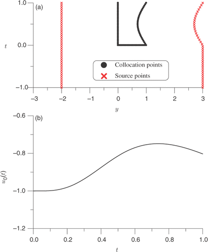
Figure 6. For Example 4: (a) the number of iterations, (b) plot of the error of mismatching to the target, and (c) comparison of the numerical solutions obtained from Section 4.2.2 with the exact one.

5.5. Example 5

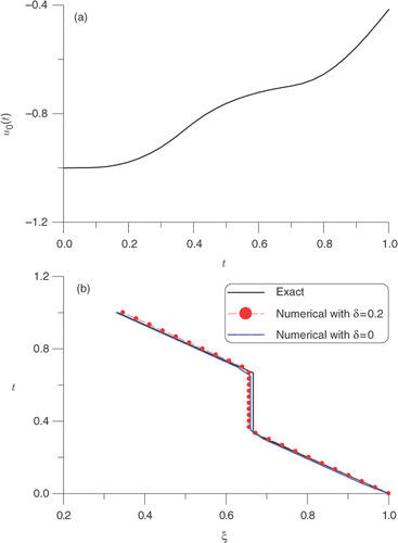
Finally, we test a rather difficult case with the exact moving boundary given by 44 (96) As that done in Example 4, the data are obtained by solving a direct problem with q₀(t) = 1, u_ξ(t) = 0 and u(y, 0) = y − 1 through the MFS. The data used in the recovery of this moving boundary are plotted in Figure 7(a). We apply the numerical method in Section 4.2.2 to solve this problem. For the non-noised input data we obtain the numerical result with a maximum error 8.94 × 10⁻⁴ as shown in Figure 7(b) by the dashed–dotted line. Even under a large noise with δ = 0.2, the recovered moving boundary is plotted in Figure 7(b) by the dashed–dotted line marked by black triangular points. The present result is better than that obtained in 44.

Figure 7. For Example 5: (a) the boundary data calculated by the MFS, and (b) comparison of the recovered and the exact moving boundaries.

Remarks

It is well-known that the inverse problem of moving boundary identification is generally ill-posed, and numerically unstable. To overcome the ill-posedness of moving boundary identification some regularization methods have been used 5,35,45–47. In the present algorithms based on the LGSM, the convergence criterion plays the role of regularization parameter. The numerical results computed by the present LGSM have some advantages that are absent by other methods, of which the main advantage is that the regularization technique of the LGSM is quite simple and straightforward. Here, we are restricted to the one-dimensional problem of moving boundary identification. The difficulties of two- and three-dimensional problems of moving boundary identification are more pronounced and only few works were reported in the literature 5,45,46. It is possible by applying the LGSM to identify the two-dimensional moving boundary, if the range of x is fixed but with y as a function of x and t, which however will be addressed in a separate paper.

6. Conclusions

In order to identify the time-dependent moving boundary under an extra measured temperature gradient on a fixed boundary, we have employed the LGSM to derive a rather simple system of linear algebraic equations. Numerical examples were worked out, which show that the LGSM can work very well even under a large noise on the measured data. Through this study, we can conclude that the new recovery method is accurate, effective and stable. Its numerical implementation is quite simple and the computational speed is fast. According to these facts, the presently proposed LGSM can be used as an accurate and effective mathematical tool to compute the unknown time-dependent moving boundary. The underlying mechanism to succeed the present recovery algorithms was that we had derived linear algebraic equations to solve the time-dependent moving boundary and the best r in the admissible range could be easily determined to fit the given right-boundary condition with only a few iterations.

Acknowledgements

The author highly appreciates the constructive comments of anonymous referees, and acknowledges the grant from Taiwan's National Science Council project NSC-99-2221-E-002-074-MY3.

References

- Fredman, TP, 2004. A boundary identification method for an inverse heat conduction problem with an application in ironmaking, Heat Mass Transfer 41 (2004), pp. 95–103.
- Evans, JD, and King, JR, 2000. Asymptotic results for the Stefan problems with kinetic undercooling, Quart. J. Mech. Appl. Math. 53 (2000), pp. 449–473.
- Beck, JV, and Arnold, KJ, 1997. Parameter Estimation in Engineering and Science. New York: Wiley; 1997.
- Hadamard, J, 1953. Lectures on Cauchy's Problem in Linear Partial Differential Equations. New York: Dover; 1953.
- Banks, HT, and Kojima, F, 1989. Boundary shape identification problems in two-dimensional domains related to thermal testing of materials, Quart. Appl. Math. 47 (1989), pp. 273–293.
- Banks, HT, Kojima, F, and Winfree, WP, 1990. Boundary estimation problems arising in thermal tomography, Inverse Probl. 6 (1990), pp. 897–921.
- Cannon, J, and Rundell, W, 1991. Recovering a time-dependent coefficient in a parabolic differential equation, J. Math. Anal. Appl. 160 (1991), pp. 572–582.
- Liu, C-S, 2001. Cone of non-linear dynamical system and group preserving schemes, Int. J. Non-Linear Mech. 36 (2001), pp. 1047–1068.
- Liu, C-S, 2006. The Lie-group shooting method for non-linear two-point boundary value problems exhibiting multiple solutions, CMES: Comput. Model. Eng. Sci. 13 (2006), pp. 149–163.
- Liu, C-S, 2006. Efficient shooting methods for the second order ordinary differential equations, CMES: Comput. Model. Eng. Sci. 15 (2006), pp. 69–86.
- Liu, C-S, 2006. The Lie-group shooting method for singularly perturbed two-point boundary value problems, CMES: Comput. Model. Eng. Sci. 15 (2006), pp. 179–196.
- Liu, C-S, 2008. A Lie-group shooting method for computing eigenvalues and eigenfunctions of Sturm–Liouville problems, CMES: Comput. Model. Eng. Sci. 26 (2008), pp. 157–168.
- Liu, C-S, 2010. The Lie-group shooting method for computing the generalized Sturm–Liouville problems, CMES: Comput. Model. Eng. Sci. 56 (2010), pp. 85–112.
- Liu, C-S, 2006. One-step GPS for the estimation of temperature-dependent thermal conductivity, Int. J. Heat Mass Transfer 49 (2006), pp. 3084–3093.
- Liu, C-S, 2006. An efficient simultaneous estimation of temperature-dependent thermophysical properties, CMES: Comput. Model. Eng. Sci. 14 (2006), pp. 77–90.
- Liu, C-S, 2007. Identification of temperature-dependent thermophysical properties in a partial differential equation subject to extra final measurement data, Numer. Methods Partial Differ. Eqns 23 (2007), pp. 1083–1109.
- Chang, CW, Liu, C-S, and Chang, JR, 2005. A group preserving scheme for inverse heat conduction problems, CMES: Comput. Model. Eng. Sci. 10 (2005), pp. 13–38.
- Chang, CW, Chang, JR, and Liu, C-S, 2006. The Lie-group shooting method for boundary layer equations in fluid mechanics, J. Hydrodyn. 18 (3) (2006), pp. 103–108, Suppl. 1.
- Liu, C-S, 2004. Group preserving scheme for backward heat conduction problems, Int. J. Heat Mass Transfer 47 (2004), pp. 2567–2576.
- Liu, C-S, Chang, CW, and Chang, JR, 2006. Past cone dynamics and backward group preserving schemes for backward heat conduction problems, CMES: Comput. Model. Eng. Sci. 12 (2006), pp. 67–81.
- Chang, JR, Liu, C-S, and Chang, CW, 2007. A new shooting method for quasi-boundary regularization of backward heat conduction problems, Int. J. Heat Mass Transfer 50 (2007), pp. 2325–2332.
- Liu, C-S, Chang, CW, and Chang, JR, 2006. The Lie-group shooting method for steady-state Burgers equation with high Reynolds number, J. Hydrodyn. 18 (3) (2006), pp. 367–372, Suppl. 1.
- Liu, C-S, 2008. An LGSM to identify nonhomogeneous heat conductivity functions by an extra measurement of temperature, Int. J. Heat Mass Transfer 51 (2008), pp. 2603–2613.
- Liu, C-S, 2008. Solving an inverse Sturm–Liouville problem by a Lie-group method, Bound. Value Probl. 2008 (2008), Article ID 749865.
- Liu, C-S, 2008. A Lie-group shooting method estimating non-linear restoring force in a mechanical system, CMES: Comput. Model. Eng. Sci. 35 (2008), pp. 157–180.
- Liu, C-S, 2008. An LGEM to identify time-dependent heat conductivity function by an extra measurement of temperature gradient, CMC: Comput. Mater. Contin. 7 (2008), pp. 81–95.
- Liu, C-S, 2009. A two-stage LGSM to identify time-dependent heat source through an internal measurement of temperature, Int. J. Heat Mass Transfer 52 (2009), pp. 1635–1642.
- Liu, C-S, 2010. A highly accurate LGSM for severely ill-posed BHCP under a large noise on the final time data, Int. J. Heat Mass Transfer 53 (2010), pp. 4132–4140.
- Murray, WD, and Landis, F, 1959. Numerical and machine solutions of transient heat-conduction problems involving melting or freezing, Trans. ASME 81 (1959), pp. 106–112.
- Finlayson, BA, 1992. Numerical Methods for Problems with Moving Fronts. Seattle: Ravenna Park Publishing; 1992.
- Liu, J, and Guerrier, B, 1997. A comparative study of domain embedding methods for regularized solutions of inverse Stefan problems, Int. J. Numer. Methods Eng. 40 (1997), pp. 3579–3600.
- Slota, D, and Zielonka, A, 2009. A new application of He's variational iteration method for the solution of the one-phase Stefan problem, Comput. Math. Appl. 58 (2009), pp. 2489–2494.
- Hon, YC, and Li, M, 2008. A computational method for inverse free boundary determination problem, Int. J. Numer. Methods Eng. 73 (2008), pp. 1291–1309.
- Liu, C-S, and Atluri, SN, 2009. A fictitious time integration method for the numerical solution of the Fredholm integral equation and for numerical differentiation of noisy data, and its relation to the filter theory, CMES: Comput. Model. Eng. Sci. 41 (2009), pp. 243–261.
- Wei, T, and Yamamoto, M, 2009. Reconstruction of a moving boundary from Cauchy data in one-dimensional heat equation, Inverse Probl. Sci. Eng. 17 (2009), pp. 551–567.
- Manselli, P, and Vessella, S, 1991. On continuous dependence, on noncharacteristic Cauchy data, for level lines of solutions of the heat equation, Forum Math. 3 (1991), pp. 513–521.
- Iserles, A, and Zanna, A, 2000. Preserving algebraic invariants with Runge-Kutta methods, J. Comp. Appl. Math. 125 (2000), pp. 69–81.
- Iserles, A, Munthe-Kass, HZ, Norsett, SP, and Zanna, A, 2000. Lie-group methods, Acta Numer. 9 (2000), pp. 215–365.
- Ying, L, and Candés, EJ, 2006. The phase flow method, J. Comput. Phys. 220 (2006), pp. 184–215.
- Liu, C-S, 2006. An efficient backward group preserving scheme for the backward in time Burgers equation, CMES: Comput. Model. Eng. Sci. 12 (2006), pp. 55–65.
- Liu, C-S, Liu, LW, and Hong, HK, 2007. Highly accurate computation of spatial-dependent heat conductivity and heat capacity in inverse thermal problem, CMES: Comput. Model. Eng. Sci. 17 (2007), pp. 1–18.
- Liu, C-S, Yeih, W, and Atluri, SN, 2009. On solving the ill-conditioned system Ax=b: general-purpose conditioners obtained from the boundary-collocation solution of the Laplace equation, using Trefftz expansions with multiple length scales, CMES: Comput. Model. Eng. Sci. 44 (2009), pp. 281–311.
- Liu, C-S, 2011. The method of fundamental solutions for solving the backward heat conduction problem with conditioning by a new post-conditioner, Num. Heat Transfer, B: Fundamentals 60 (2011), pp. 57–72.
- Liu, C-S, 2011. Solving two typical inverse Stefan problems by using the Lie-group shooting method, Int. J. Heat Mass Transfer 54 (2011), pp. 1941–1949.
- Huang, CH, and Chao, BH, 1997. An inverse geometry problem in identifying irregular boundary configurations, Int. J. Heat Mass Transfer 40 (1997), pp. 2045–2053.
- Huang, CH, and Tsai, CC, 1998. A transient inverse two-dimensional geometry problem in estimating time-dependent irregular boundary configurations, Int. J. Heat Mass Transfer 41 (1998), pp. 1707–1718.
- Liu, C-S, Chang, CW, and Chiang, CY, 2008. A regularized integral equation method for the inverse geometry heat conduction problem, Int. J. Heat Mass Transfer 51 (2008), pp. 5380–5388.