Abstract
Land surface and ecosystem processes affect climate and weather in a range of time scales, from seconds to thousands of years. Land surface/ecosystem models (LSEMs) calculate the fluxes between the biosphere and the atmosphere and other ecosystem dynamics processes. In this study, we develop a calibration procedure, based on the theory of ecosystems hierarchy, to optimize all processes simulated by an LSEM. The procedure was implemented on Optis, a software for hierarchical multi-objective calibration of LSEMs. Optis is based on the multi-objective genetic algorithm, Non-dominated Sorted Genetic Algorithm-II (NSGA-II). The calibration was hierarchically performed from the fastest process (radiative fluxes) to the slowest process (carbon allocation), optimizing nine model outputs. The procedure demonstrated to be efficient, with the nine-objective model optimization reaching about 80% of the performance achieved by the mono-objective optimization. This calibration methodology allows a better global performance of the model, as all simulated variables are optimized.
Nomenclature
| B | = | intercept of the linear regression between simulations and observations |
| Bmax | = | maximum bias during the simulation period |
| D | = | relative performance index |
| fAPAR | = | fraction of absorbed photosynthetically active radiation (dimensionless) |
| GA | = | genetic algorithm |
| H | = | sensible heat flux (W m−2) |
| IBI | = | integrated biosphere simulator |
| LAI | = | leaf area index (m2 m−2) |
| LE | = | latent heat flux (W m−2) |
| Lin | = | incident long-wave radiation |
| LSEM | = | land surface/ecosystem model |
| M | = | slope of the linear regression between simulations and observations |
| MAE | = | mean absolute error |
| NEE | = | net ecosystem exchange (µmol m−2 s−1) |
| NPP | = | net primary productivity (kg-C m−2 year−1) |
| NSGA-II | = | Non-dominated Sorted Genetic Algorithm-II |
| O | = | observed data |
| P | = | predicted data |
| Prec | = | precipitation (mm h−1) |
| PARo | = | reflected photosynthetically active radiation (µmol m−2 s−1) |
| Q | = | air humidity |
| RMSE | = | root mean squared error |
| Rn | = | net radiation (W m−2) |
| SA | = | sensitivity analysis |
| Sin | = | incident short-wave radiation flux |
| T | = | air temperature (K) |
| U | = | wind speed (m s−1) |
| u* | = | friction velocity (m s−1) |
| μ | = | mean effect of the model output parameters (Morris measure) |
| μ* | = | absolute value of μ |
| σ | = | non-linear or interactions effects that involve model output parameters (Morris method) |
| σ | = | Stefan–Boltzmann constant on Equation (6) |
1. Introduction
Terrestrial ecosystems are a key component for the study of Earth climate. There are evidences that land surface processes affect climate and weather in a range of time scales, from seconds to millions of years Citation1–4.
Land surface/ecosystem models (LSEMs) simulate the processes of terrestrial ecosystems and are an important tool for research on climatic simulations and weather forecast, generally working coupled to atmospheric general circulation models and acting as submodels calculating micrometeorological processes such as radiation, heat, water vapour and momentum fluxes through the biosphere–atmosphere interface.
LSEMs have become increasingly complex as both terrestrial ecosystems’ functioning knowledge and computer power increase, allowing new processes to be represented by the models. Hence, models are evolving to incorporate not only micrometeorological processes (mass, energy and momentum fluxes), but also vegetation dynamics and terrestrial carbon balance processes. At the same time, intensive data collection at field sites concurrently obtains not only flux data, but also several other ecosystem measurements, including rate of biomass growth and seasonal variations in leaf area index (LAI). In many intensive field sites, it is common to have over 10 observations available that could be used to optimize model performance, although recent optimization studies usually have used only two or three of these observation data sets.
The main objective of this article is to propose and evaluate a methodology to calibrate an LSEM, or optimize the model performance of unlimited variables, against available matching field observations.
Many processes are represented on LSEMs through the use of several parameters, some of which must be calibrated by optimization procedures to minimize differences between model results and observed data. Each variable simulated by the model represents at least one objective of the optimization problem. Thus, calibrating several output variables model means to identify a parameter set that minimizes a vector of objective functions simultaneously, i.e.
(1)
in which f1(θ), … , fn(θ) are the different n objective functions to be simultaneously minimized (usually, they measure the difference between observations (O) and corresponding variable simulated (P)), θ is the set of model parameters and Θ is the constraint set, which may either be explicitly given or implicitly defined Citation5. θ includes not only the full set of model parameters, but also the range in which each parameter is allowed to vary. The solution to the above problem is a set of Pareto points. Pareto solutions are those for which improvement in one objective can only occur with the worsening of at least one other objective. Thus, instead of a unique solution to the problem (which is typically the case in mono-objective optimization problems), the solution to a multi-objective problem is a (possibly infinite) set of Pareto points, also called a Pareto frontier.
The choice of adjustment metrics between simulations and observation for model calibration is of great relevance, apparently greater than the choice of the optimization method itself Citation6. Adjustment metrics define objective functions on the context studied, and shall provide a single scalar value to indicate simulated data quality in relation to observed data. Reliable results may require more than one adjustment metric to be optimized simultaneously. In this case, optimization of a single-model output variable already configures a multi-objective optimization problem, with each adjustment measure representing an objective function.
Since the early days of optimization science, it has been recognized that calibrating a complex model, affected by many parameters and multiple objective functions, can be particularly difficult to be done accurately and efficiently Citation7–10. The difficulty of an optimization problem usually is related to three major factors:
| 1. | Number of parameters of the problem: as the number of parameters to be optimized grows, the search space and the actual effort to achieve the global optimum also grow. | ||||
| 2. | Objective function features: the surface of the objective functions on the parameters space may be neither smooth nor continuous. Furthermore, there might be several regions of attraction, each one containing many local minima Citation10,Citation11. | ||||
| 3. | Number of objective functions: it is usual to consider, for results evaluation, more than one output variable, or even a single variable using more than one statistic. This multi-objective feature makes the calibration process more complicated, because conflicts among the objectives are frequent Citation12. | ||||
An effective sensitivity analysis (SA) can decrease the difficulty presented in (1). Using the more sensitive parameters detected by an SA can reduce the search space and allow a more efficient optimization. Global search techniques, called metaheuristic, are necessary to solve the problem described in (2), as they are capable of providing good solutions to these problems. Multi-objective optimization algorithms are required to deal with multiple objective functions, since they are able to provide sets of solutions to satisfy all the objectives simultaneously. Nevertheless, an excessively large number of objectives might make the optimization problem unfeasible. In that case, the problem objectives must be reduced somehow, for example, by dividing the problem into several sub-problems with fewer objectives, or as grouping several objectives within a single function to be minimized.
Several methodologies were proposed for more precise and realistic LSEM calibration. However, no calibration method currently in use allows satisfactory calibration to every output of complex models, even when observations are available. Most calibration methods developed optimize no more than three objective functions (n ≤ 3) simultaneously Citation12–16.
In this study, we propose a calibration procedure for the optimization of the multiple outputs of recent land surface/dynamic vegetation models. To overcome the performance degradation for n > 3, we propose a hierarchical approach, in which the processes simulated by the model are organized in hierarchical levels and, at each level, up to three objective functions are simultaneously optimized by a standard multi-objective optimization technique.
The core of this proposed methodology uses evolutionary algorithms for optimization. Evolutionary algorithms are frequently applied to complex models optimization problems Citation13,Citation14,Citation17–19. Such algorithms provide a global search in the parameter space, avoiding the local optimum convergence problem. Moreover, they grant a multi-objective optimization based on the Pareto frontier concept, resulting in a set of possible optimum solution representing exchanges between the conflicting objectives. This allows the researcher to choose the best solution within the algorithm output set, following previously established criteria.
In addition, the proposed methodology is based on environmental systems hierarchy to simultaneously calibrate all variables simulated by recent LSEMs that have corresponding field observations. The calibration is hierarchically made from fast processes (radiation fluxes) to slow processes (carbon allocation).
We test the procedure on the Integrated Biosphere Simulator (IBIS) Citation20. IBIS is a fourth-generation LSEM that simulates exchanges of mass and energy between the vegetation and atmosphere, plant physiology and photosynthesis, phenology, carbon allocation, vegetation dynamics and the full terrestrial carbon cycle.
The procedure has four steps: (a) first, an SA is run to select, efficiently, the more important parameters for each model output. The SA uses the Morris method Citation21, with the calculation of the sensitivity index modified to satisfy LSEMs; (b) an automatic multi-objective calibration software for the IBIS model was developed, called Optis, based on Non-dominated Sorted Genetic Algorithm-II (NSGA-II) multi-objective genetic algorithm (GA) Citation22. This algorithm allows the simultaneous optimization of multiple metrics and several model outputs; (c) third, the LSEM hierarchical calibration methodology was applied to perform calibration in all simulated processes of the model that had matching observations; (d) finally, the model hierarchical calibration is compared to independent mono-objective calibrations of each variable, which are considered to be the best calibrations possible, and the comparison of both calibrations provides a relative performance index of the proposed calibration method. We expect that the hierarchical calibration will provide a well-adjusted simulation of all processes represented by the model.
This article is divided into five parts. In Section 2, we present a literature review on several optimization concepts. Section 3 presents a description of the model used, the site and data used for evaluation, filtering procedures, the evolutionary optimization algorithm and the hierarchical procedure used to optimize the model. We also introduce the relative performance index, which we later use to evaluate the hierarchical procedure. Section 4 presents the results and algorithm evaluation. Sections 5 and 6 present a final discussion, conclusions and recommendations for future work.
2. Literature review
2.1. Sensitivity analysis
SA is the study of the relation between input and output data of a model. Through SA it is possible to understand how variability in the model output may be attributed to the variability in the input. The aim of SA is to investigate how a computer model responds to parameters variations, determining:
| 1. | the insignificant parameters of the model for a specific output, so they can be disregarded during calibration process, | ||||
| 2. | the optimum region of parameters space to be used in the subsequent calibration study and | ||||
| 3. | whether and which parameters interact with each other. | ||||
The elimination of insignificant parameters in some outputs (1) allows a reduction in the dimensions of the parameters space and makes the search process easier. An investigation of the whole parameters space is necessary, i.e. a global SA (2). Frequently, parameters interact and have combined effects that cannot be reduced to the sum of individual effects (3), which is relevant since it influences items 1 and 2.
2.1.1. Types of SA
There are three classes of SA methods: screening methods, local SA methods and global SA methods Citation23.
Screening experiments are used to identify the parameters set that are responsible for most of the model output variation. Since they are computationally inexpensive, they usually are fit to work with high computational costs and large number of parameters. They are based on the principle that parameters influence on models following Pareto law (80% of consequences arise from 20% of causes), with most parameters non-influent. On the other hand, these methods tend to provide qualitative sensitivity measures, i.e. they arrange the input factors in the order of importance but do not quantify how much a parameter is more important than another. In contrast, a quantitative SA method may inform, for example, the exact percentage of the total output variance that each parameter is responsible. In screening methods, the exchange between computational cost and information is clear.
Local SA is a quantitative SA that focuses on the local impacts of model parameters. Usually, such analysis is made by the partial derivative calculation of model output functions related to input parameters. They vary around a nominal value in a small interval to calculate these derivatives numerically. The SA is a singular one-factor-at-a-time approach, since one factor varies while the whole factor set is constant. These local SA methods are effective in selecting the most important parameters only when all model parameters are linear, and the model is monotonic Citation24.
Global SA techniques proportionally associate model outputs uncertainties to input parameter uncertainties. Sensitivity estimates for each parameter consider its whole variation interval and they are developed varying all other parameters as well. Hence, it is possible to calculate individual effects from each parameter and interaction effects between parameters or parameters sets.
2.1.2. Morris method
The SA method proposed by Morris Citation21 is a screening method, developed to deal with models containing large amount of parameters or high computational costs. The aim of this method is to find out which parameters, within a set of several potentially important parameters, are indeed relevant. Morris method intends to identify which parameters effects are (a) negligible, (b) linear and additive or (c) non-linear or involved in interactions with other factors.
This method essentially consists of varying one parameter at a time. Each parameter may assume a discrete number of values, called levels, chosen within the parameters variation interval. Two sensitivity metrics are proposed by Morris: measure μ that estimates the mean effect of the model output parameters, and measure σ that, through the standard deviation, estimates second and higher order effects that involve the parameter (non-linear effects and interactions included). The Morris sensitivity measure, called elementary effect, uses incremental variations on the parameters, like a local SA. However, the final measure μ is obtained through the mean of several elementary effects, calculated in different points of the parameter space. Thus, it is independent of the specific points in which the elementary effects are calculated. This method tends to explore several regions of the parameter space, and therefore may be considered a global SA method.
A third measure μ* Citation24 is a modular version of Morris measure, i.e. the absolute value of elementary effects. This measure avoids a Morris method flaw regarding non-monotonic models. In such case, opposite sign elementary effects could occur and cancel each other at the mean calculation, providing a low μ value.
2.2. Model evaluation
The number and types of meteorological and environmental models are growing, increasing the need for effective evaluation and validation techniques for such models, since validation is an essential modelling step. Many authors discuss which formulations and error metrics are more adequate to verify model accuracy and effectiveness Citation25–30.
A model evaluation is performed by comparing predicted results with observed values for the analysed variable. Such comparison is usually obtained through numerical values output metrics representing how well-simulated data fits observed data. Thus, the importance of the choice of the adequate statistics for proper model evaluation is evident.
The choice of adjustment metrics is also a critical factor for the model calibration, even more important than the selection of optimization method Citation6. In this sense, the evaluation of the model can be seen as one of the steps of the calibration procedure, since several evaluations of model results may be performed in the search for optimal values to parameters.
2.2.1. Models statistics and adjustment metrics
Several statistics and techniques are referred to in the literature and used for error determination between observed data (O) and predicted data (P). Among them are Pearson correlation coefficient (r), coefficient of determination (r2), mean absolute error (MAE), root-mean-squared error (RMSE), Nash-Sutcliffe efficiency coefficient (E), Willmott Agreement Index (d), and m and b linear regression coefficients (slope and intercept) for simulated data versus observed data Citation13,Citation18,Citation25,Citation28,Citation30,Citation31. Mean error metrics (e.g. RMSE and MAE) provide appropriate and comprehensible information on model adjustment to observed data. Within these metrics, RMSE and MAE are particularly interesting since they are dimensional metrics, i.e. they state the model error in the same unit as the analysed variable. The model evaluation procedures should report at least one of these metrics Citation27. Even though they express error on the same unit as the analysed data, these two statistics possesses some features that differentiate them. RMSE depends on error magnitude variability (or quadratic error), on n1/2 and on mean error magnitudes. Therefore, without additional information (e.g. MAE), it is impossible to distinguish how much from RMSE represents central tendency (mean error) and how much of it represents n1/2 or quadratic error distribution variability (RMSE limit is given by MAE ≤ RMSE ≤ MAE.n1/2 Citation29). MAE is a more natural mean error metric, as its formula requires neither quadratic terms nor roots. Different from RMSE, MAE is not ambiguous – it conveys the mean errors in absolute values. Since it is clearer to interpret, MAE is more appropriate to method evaluation, instead of RMSE or its related metrics. MAE and RMSE are given by:
(2)
(3)
Another measure of error, orthogonal to MAE and RMSE, is the bias, or the difference between the model cumulative output and the corresponding cumulative observed data. For a series of length n, the bias B is given by:
(4)
B only evaluates the bias for the entire simulation period. However, models can be unbiased at the end of the period of simulation, but be biased during the simulation, so a more robust metric is the maximum bias (Bmax) during the simulation period:
(5)
2.3. GAs applied to optimization problems
A heuristic method is, in general, a good solution for a given complex problem Citation32. Heuristic can be understood as an approximation protocol or algorithm, reducing or limiting search for solutions within difficult and little comprehended domains. A heuristic algorithm provides solutions without a formal quality limit, and is empirically evaluated regarding quality of solutions. Metaheuristics go beyond this concept, based on ideas and concepts from other disciplines as an aid to solve problems Citation33.
GAs Citation34 are metaheuristics based on Darwin's theory of evolution, which simulate natural selection and the survival of the fittest. GAs search for a good solution to a problem by randomly generating a set of potential solutions and by influencing these solutions through genetic operators. Genetic operators develop new solutions from the existing ones, supposedly better than the previous. GA terminology conveys that a solutions population is generated and refers to each solution as a gene (or individual in a population). A scalar aptitude value is determined to each individual, like a numerical representation for its problem-solving fitness. The main idea is to select the fittest solutions for reproduction and generate new individuals from them by applying genetic operators. By mutation and crossover operations, fittest individuals are expected to be generated outside the current set of potential solutions. This process continues until an acceptable solution is obtained.
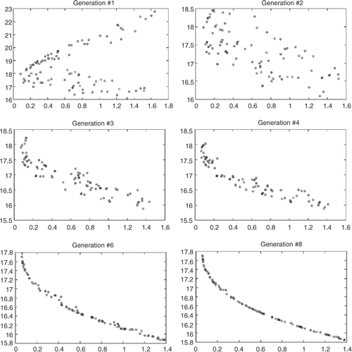
In a multi-objective GA, individuals present multiple aptitude functions that must be simultaneously evaluated during the fittest individual selection process. Individuals are selected aiming to develop a slope or surface in the objectives space, called Pareto frontier. In this frontier, all individuals are equally apt, and a simple optimum solution choice shall be done either from subjective or empirical criteria, or in concordance with previously defined priorities Citation35. The evolution of a multi-objective GA and the Pareto frontier construction are illustrated in , using the problem ZDT4, one of the mathematical problems suggested by Zitzler et al. Citation36 to evaluate multi-objective GAs.
3. Methodology
3.1. The IBIS model
The IBIS model was designed to connect land and hydrologic processes, land biogeochemistry cycles and vegetation dynamics into a single modelling framework Citation20. The model includes representations of surface physical processes (including solar radiation transfer through the canopy, turbulent processes, water interception by canopy, heat and mass transfer by canopy), plant physiology, canopy phenology, vegetation dynamics for different plant functional types, carbon allocation and soil biogeochemistry. All processes are organized in a hierarchical form and operate on different time scales, ranging from minutes to years.
The model has 43 input parameters, chosen by their significance in defining physical, physiological or biogeochemical processes. Thus, some of them are not independent. For more details on the parameters, refer to Citation20.
3.2. Site description and observed data
For IBIS model calibration, we used data collected at an Amazon micrometeorological site: the km 67 Tapajós National Forest. This site is located near the km 67 of Santarém-Cuiabá highway (2°51, 54°58′W), south from Santarém, Pará, Brazil. The typical land cover is evergreen tropical rainforest, in flat terrain, formed mainly by evergreen and some semideciduous species. The forest spans 5 km to the east, 8 km to the south and 40 km to north, before it bordering pasture Citation37. Canopy height is 40 m, on average, with emerging trees reaching up to 55 m.
Observed data from the experimental site were used as input for IBIS and for results validation. Model input includes air temperature (T) and specific humidity (q), precipitation (Prec), wind speed (u), short- and long-wave incoming radiation fluxes (Sin, Lin).
Tapajós National Forest data were collected in the following periods: reflected photosynthetically active radiation (PARo), net radiation (Rn), friction velocity (u*), sensible heat flux (H), latent heat flux (LE), net ecosystem exchange (NEE) and model inputs are hourly means, from January 2002 to December 2004. Net primary productivity (NPP) is a single-value (annual mean for 2004) fraction of absorbed photosynthetically active radiation (fAPAR) and LAI are monthly means for 2002 and 2004, respectively Citation38,Citation39. The model was calibrated for nine variables: PARo, fAPAR, Rn, u*, H, LE, NEE, NPP and LAI.
Latent and sensible heat fluxes were measured by an eddy covariance system. Surface radiation budget, air temperature and humidity, wind speed and other variables were measured by an automatic micrometeorological station Citation37. Incident long-wave radiation data (Lin) were not collected at the experimental site. Hence, Lin was estimated by
(6)
where
is the canopy emissivity and
is the Stefan–Boltzmann constant.
3.2.1. Data gap-filling
The gaps in the observed data used as IBIS input were filled using interpolation Citation38.
If the number of gap points (g) is less than or equal to 3 h, we use:
(7)
where Xi is the value to be filled, Xp is the gap predecessor and Xp + g + 1 is the gap successor; i is the cell index that will be interpolated and p is the cell index that precede the gap.
If the gap duration is greater than 3 h and less than 24 h:
(8)
If the gap duration is greater than or equal to 24 h:
(9)
where m is the integer part of
.
These interpolation equations make the behaviour of the period without data similar to the period with data. Thus, the gaps are filled in a more realistic way than the linear interpolation, except for g ≤ 3 h.
3.2.2. Data filtering before model evaluation
This study used three types of data filtering before the model calibration Citation40,Citation41: Filtering based on the missing input data, on the threshold of friction velocity, and on energy budget closure.
The first filter eliminates of the model evaluation process the periods when there were gaps in the input data series, which were filled. This filter aims to remove from the analysis the effects of any inconsistencies in the filled input data.
NEE filtering by friction velocity eliminates of the model evaluation processes the period when there was low turbulence during the flux measurements (u* < 0.1 ms−1). In low-turbulence conditions, CO2 flux cannot be correctly measured by the eddy covariance technique, and measurements are usually underestimated Citation37.
Filtering based on energy budget closure eliminates of the model evaluation processes the days when the energy budget closure is poor (Rn − LE − H > ε.Rn). A fundamental problem of measured eddy covariance data is that the data do not always indicate energy closure. The sum of sensible and latent heat fluxes usually underestimates the net radiation by, at least, 20% Citation42. This study used ε = 0.4, i.e. we considered only the periods of data whose daily energy budget measured by eddy covariance was within 40% of the budget energy measured by radiative instruments Citation40,Citation41.
3.3. Multi-objective calibration
The LSEM calibration problem may be seen as a multi-objective calibration problem from different perspectives. One perspective is that several variables simulated by the model can be simultaneously calibrated, and in that case, each variable adjustment becomes an objective to the optimization problem.
Another way is to simultaneously optimize more than one statistic or error metric for a variable simulated by the model. In this case, each adjustment metric of the analysed variable becomes an objective to the optimization problem.
A third possibility is to merge both approaches, seeking calibration of several simulated variables through the simultaneous optimization of a statistics set. In that case, there is an optimization problem with an excessively large number of objectives, possibly insoluble.
In this study, we developed Optis, an IBIS multi-objective optimization software. Optis can be used to deal with any of the calibration types stated above, and is based on NSGA-II multi-objective calibration algorithm Citation22. NSGA-II is a revised and improved version for one of the first multi-objective GAs, the NSGA Citation43.
NSGA-II algorithm is based on the Pareto frontier concept, in order to find optimal solutions for multi-objective optimization problems. After defining the Pareto frontier solutions set, Optis returns the output as the best solution that symmetrically optimizes all the objectives, i.e. it selects the solution that is closest to the origin. Hence, an equal weight is assumed to all objectives. This characteristic was arbitrarily chosen and can be modified with minimal changes to the algorithm itself.
To avoid interference from objective function units or value scales, normalization of the algorithm output is performed before the choice of the optimal value. By doing so, all objective values of the simulated solutions (Pareto frontier) will range between zero and one. Thereafter, the point with the smallest Euclidean distance from the origin is selected as the best solution for the optimization problem.
The algorithm has limitations to work with large number of objectives, which is loss of optimization efficiency while dealing with more than three objectives at once. This is an NSGA-II algorithm limitation Citation44. Even with a population size increase, NSGA-II provides bad results with large number of objectives Citation45. Thus, in this study, multi-objective calibrations were constrained to at most three simultaneous objectives.
3.3.1. Optis’ structure
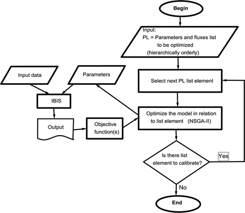
Optis was based on the language C code of NSGA-II software and it was developed to work coupled with IBIS model, optimizing its parameter values automatically. During the calibration process, IBIS independently operates from Optis and is run without the optimization algorithm (). The optimization algorithm interacts with the model only through reading output data and changing input data parameters. In that way, Optis is practically independent from the IBIS version or even from the model to be calibrated itself. Just a small change in the IBIS reading protocol was necessary to simplify the parameters reading and writing process for Optis and IBIS.
Optis is absolutely configurable and allows infinite types of calibration experiments, enabling the calibration of any combination of simulated variables by the model, the use of any adjustment metrics and the calibration of any combination of the 43 model parameters. Furthermore, it is possible to sequentially perform independent calibrations from IBIS, allowing several model variables to be calibrated one after another, keeping each and every parameter calibration output.
3.3.2. Calibration algorithm test
Two IBIS multi-objective calibration tests were developed to test and validate Optis program. In the first test, a model variable (LE) was independently calibrated, considering two adjustment metrics as objectives (MAELE and ). In this case, the problem multi-objectiveness is related to the amount of adjustment metrics (two adjustment metrics imply two objectives).
In the second multi-objective calibration test, two model variables (H and LE) were simultaneously calibrated for a single-adjustment metric (MAEH and MAELE). The algorithm optimized the parameters finding possible values for both variables simultaneously, each one with the same weight as the other. In that case, the problem multi-objectiveness relates to the number of adjusted model variables (two variables imply two objectives).
For the performance evaluation of optimization algorithm using multiple objectives, the multi-objective calibrations were compared to the respective mono-objective calibrations. In the mono-objective calibrations, each variable is exclusively optimized, i.e. in each calibration, all the parameters are calibrated to optimize a single variable. Thus, the mono-objective calibration results can be assumed the best results possible.
To evaluate the general adjustment of the model obtained by the multi-objective calibration, a relative performance statistic (D) was calculated, measuring multi-objective calibration performance in relation to mono-objective calibration. After the multi-objective calculation, D is calculated as the mono-objective and multi-objective ratio for each optimized objective function. These individual values display how close each objective is from its best value (mono-objective calibration). The D index is calculated by the average of all mono-objective/multi-objective ratios. D should be smaller than the unit, and the higher the value of D, the higher is the multi-objective calibration efficiency in relation to the mono-objective optimization.
The relative performance index is defined by the formula:
(10)
in which fmono is the objective function used to evaluate the model subjected to mono-objective calibration, fmulti is the objective function used to evaluate the model subjected to multi-objective calibration and n is the number of objective functions.
3.4. Multi-objective hierarchical calibration
To obtain LSEM-intended performance, the model should be calibrated in a way that all the processes are realistically simulated. However, calibrating the several LSEM-simulated processes within a single multi-objective optimization experiment would be infeasible, due to the large number of objective functions considered simultaneously. This large number depends on the available field observations and varies from site to site.
Environmental systems are complex and their processes are organized by several space and time scales Citation39,Citation46. LSEMs usually are hierarchically organized and represent processes that occur in many different scales Citation47. For instance, IBIS Citation20 simulates processes that span through a range of time scales, from energy and mass fluxes (time scale: seconds) to carbon budget in soils and vegetation dynamics, including competition between plant functional types (time scale: decades). Therefore, model parameters are related to several different processes and diverse temporal scales. Each parameter can influence one or more processes at a single time scale or influence processes at different scales.
This study intends to use a temporal hierarchical approach to separately calibrate each process, or set of processes, according to its hierarchical level. Thus, it was possible to calibrate 43 model parameters, optimizing nine output variables.
The hierarchical level is defined by simulated processes’ temporal hierarchy, from faster processes to slower ones. Short-wave radiation fluxes were calibrated in the first hierarchical level, surface radiation budget in the second, turbulence in the third, turbulent fluxes in the fourth and variables related to carbon allocation in the fifth and last levels. The method allows calibration of unlimited objective functions and output variables, distributed in any arrangement of hierarchical levels, as long as it does not exceed three objective functions per hierarchical level.
Through SA and previous knowledge about the relationship between simulated parameters and processes, the parameters related to each IBIS’ output variables were grouped. Thereby, each process (or groups of processes) was calibrated as an independent procedure, reducing the amount of objective functions in each calibration sub-procedure. The output values from each hierarchical level are kept in the next levels, resulting in a full adjustment for the whole set of parameters at all levels.
Model calibrations were made for the Tapajós National Forest km 67 site for the period of January 2002 to December 2004. The hierarchical levels of calibration and the optimized output were defined as
Level 1: PAR fluxes: PARo and fAPAR | |||||
Level 2: Radiation fluxes: Rn | |||||
Level 3: Turbulence: u* | |||||
Level 4: Turbulent fluxes: NEE, H and LE | |||||
Level 5: Carbon allocation: LAI and NPP. | |||||
In the hierarchy level 2, which contains a single model output variable, it is possible to apply both adjustment metrics (MAE and Bmax). In the remaining levels, only MAE was applied, in order to respect the constraint of three objective functions per level. In level 3, although only one output was optimized, we did not use Bmax, because this is an objective function more oriented to cumulative fluxes. presents the objective functions and the calibrated parameters by hierarchical level.
Table 1. Objective functions and calibrated parameters at each hierarchical level.
Each variable was also exclusively optimized on mono-objective calibrations, i.e. for each calibration, all parameters were calibrated to optimize a single variable. The hierarchical calibration results were compared with calibration reference values for each variable, obtained from the mono-objective calibration results for the respective variables.
For general adjustment evaluation of the obtained model in hierarchical calibration, the D relative performance statistic was calculated, similar to the one calculated on multi-objective calibration evaluation (Section 3.3.2). Thus, the hierarchical calibration performance was evaluated using mono-objective calibrations as reference.
For hierarchical calibration, the relative performance index is defined by
(11)
in which fmono is the objective function applied to evaluate the model subjected to mono-objective calibration, fh is the objective function applied to evaluate the model subjected to hierarchical calibration and n is the number of objective functions.
4. Results and discussion
4.1. Calibration algorithm test
compares the multi-objective calibration results with multiple statistics for the LE output variable. As expected, the best MAE value is obtained by minimizing its own objective {MAELE} (the name in {} indicates a reference to the optimization problem objective, not to the variable value). Likewise, the best Bmax value is obtained by the objective optimization {}. The multi-objective optimization {MAELE,
} solution is intermediate between the results for MAE and Bmax found in the mono-objective optimizations. This result is consistent with the Pareto curve behaviour, i.e. during multi-objective optimization, there was an exchange between optimal values of the objective functions.
Table 2. MAE and Bmax of simulated and observed LE data and mono-objective/multi-objective ratio used to calculate D index.
According to mono-objective/multi-objective ratio, the multi-objective calibration results for MAE and Bmax are very close to its mono-objective calibration, with D = 0.92. Therefore, the multi-objective optimization algorithm was indeed efficient on multiple error metrics calibration.
shows results from the second multi-objective calibration test {MAEH, MAELE}. As in the first algorithm test, the objectives {MAELE} and {MAEH} are conflicting with each other, i.e. one is minimized while the other increases. Optis was also efficient in finding an optimum intermediate value for both variables when simultaneously optimized, obtaining D = 0.93.
Table 3. MAE of simulated and observed H and LE data and mono-objective/multi-objective ratio used to calculate D index.
These results demonstrate that Optis is efficient in solving multi-objective calibration problems, obtaining a multi-objective calibration performance greater than 90% of the performance obtained during mono-objective calibration.
4.2. Mono-objective calibration (not hierarchical)
presents MAE and Bmax mono-objective calibration results. Figures show model simulation results after mono-objective calibration for each variable and compare the simulated data to observed data.
Figure 3. Results of PARo after mono-objective calibration. The graphs represent (a) sample of 10-day series data, (b) cumulative sum, (c) typical day and (d) scatter plot.
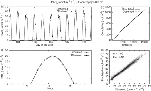
Figure 4. Results of fAPAR after mono-objective calibration. The graphs represent (a) a year of monthly data and (b) scatter plot.

Figure 5. Results of Rn after mono-objective calibration. The graphs represent (a) sample of 10-day series data, (b) cumulative sum, (c) typical day and (d) scatter plot.
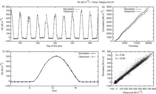
Figure 6. Results of u* after mono-objective calibration. The graphs represent (a) sample of 10-day series data and (b) scatter plot.

Figure 7. Results of H after mono-objective calibration. The graphs represent (a) sample of 10-day series data, (b) cumulative sum, (c) typical day and (d) scatter plot.
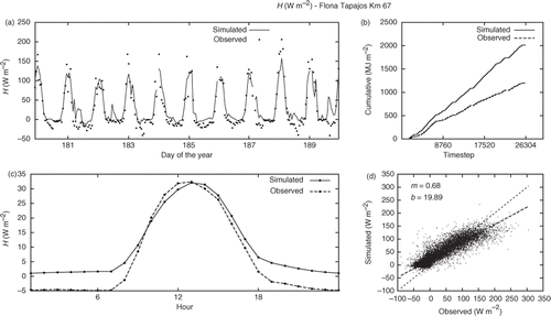
Figure 8. Results of LE after mono-objective calibration. The graphs represent (a) sample of 10-day series data, (b) cumulative sum, (c) typical day and (d) scatter plot.
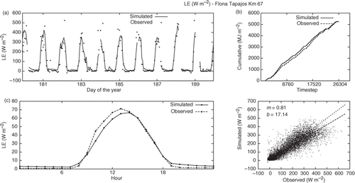
Figure 9. Results of NEE after mono-objective calibration. The graphs represent (a) sample of 10-day series data, (b) cumulative sum, (c) typical day and (d) scatter plot.
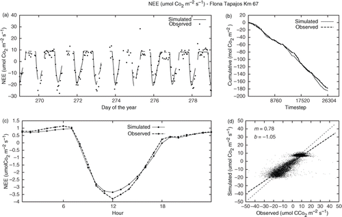
Figure 10. Results of LAI after mono-objective calibration. The graphs represent (a) a year of monthly data and (b) scatter plot.

Table 4. Results of the hierarchical calibration in the Tapajós National Forest km 67 site and the mono-objective calibration (reference values).
presents the mono-objectively calibrated PARo. The graphs indicate an almost perfect adjustment on PARo hourly data and a linear regression coefficients m = 1.00 and b = −0.12.
shows the simulated fAPAR after the mono-objective calibration. Despite the good fit between monthly observed and simulated data (), the linear regression coefficients do not display good values, influenced by the small data variability.
presents the mono-objectively calibrated Rn results. Rn-simulated data are well-adjusted to observations and a nearly perfect linear regression line is verified. Observing a typical day (), simulated Rn slightly overestimates observations during the night, which can also be noted in the cumulative sum graph (). Lin estimate methodology (Equation 6) may be the cause of this error.
shows u* after mono-objective calibration. An underestimation of the high values and an overestimation of the small values can be observed. This could indicate a deficiency in the simulation of the turbulence correction for stable and unstable atmospheric conditions, which were not calibrated. This deficiency shall affect the model ability to simulate turbulent fluxes, which are described below.
presents H results after mono-objective calibration. A sharp bias between observed and simulated data is observed (), resulting from the overestimated flux during the night, when the model could not simulate the negative H values adequately. This could be a consequence of the incorrect simulations of night time Rn (). Even though reaching some observed peaks was not possible (), the highest H values were, on average, well-simulated by the model throughout the analysed period ().
presents the calibrated LE by the mono-objective method. The simulated LE was well-adjusted to the observed LE, with a slight bias between the cumulative sum curves. The model had some difficulty in LE peaks’ simulation (), which can also be noted in the linear regression ().
presents the NEE result after mono-objective calibration. The simulated NEE was well-adjusted to the observed fluxes, with a satisfactory long-term adjustment () and a well-adjusted mean hourly behaviour (). However, the slope m in linear regression is smaller than the unit, probably a consequence of u* simulation deficiency.
The annual NPP simulated value was identical to the only observed value available (1.055 kg-C m−2 year−1).
Finally, shows calibrated LAI by the mono-objective method. The m and b coefficients for linear regression scatter plot are poor, despite the good adjustment observed in . This indicates that linear regression coefficients should be used with caution for model evaluation and calibration. These coefficients ought to be used as complementary analysis to other adjustment metrics.
4.3. Multi-objective hierarchical calibration
presents IBIS hierarchical calibration results for Tapajós National Forest site. The objective values optimized by hierarchical calibration are compared to mono-objective calibrated values for each variable.
The relative performance index was D = 0.721, considering 10 optimized objective functions from a total of 9 calibrated outputs. This D result was influenced by the bad result of NPP ratio mono-objective/hierarchical. The obtained value for this ratio, zero, does not properly represent the good adjustment settled for hierarchically calibrated NPP. Even though MAE of hierarchical calibration displayed a small value, the perfect adjustment obtained on mono-objective calibration (MAE = 0.000) reduces NPP ratio mono-objective/hierarchical to zero, forcing down the mean value of D. Such perfect adjustment of calibrated NPP through mono-objective mode is a direct result of a single observed value for annual NPP.
Excluding NPP from the procedure, the D statistic becomes 0.801, which is a more realistic value, since it is not influenced by the false bad performance of NPP from mono-objective/hierarchical ratio.
Figures display results from calibrated variables simulations by the hierarchical method and compare simulated to observed data.
Figure 11. Results of PARo after hierarchical calibration. The graphs represent (a) sample of 10-day series data, (b) cumulative sum, (c) typical day and (d) scatter plot.
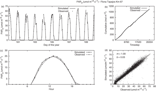
Figure 12. Results of fAPAR after hierarchical calibration. The graphs represent (a) a year of monthly data and (b) scatter plot.

Figure 13. Results of Rn after hierarchical calibration. The graphs represent (a) sample of 10-day series data, (b) cumulative sum, (c) typical day and (d) scatter plot.
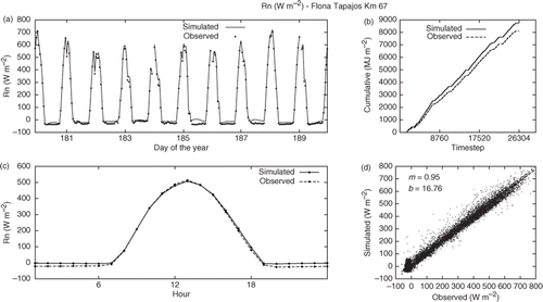
Figure 14. Results of u* after hierarchical calibration. The graphs represent (a) sample of 10-day series data and (b) scatter plot.

Figure 15. Results of H after hierarchical calibration. The graphs represent (a) sample of 10-day series data, (b) cumulative sum, (c) typical day and (d) scatter plot.
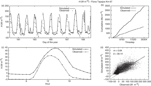
Figure 16. Results of LE after hierarchical calibration. The graphs represent (a) sample of 10-day series data, (b) cumulative sum, (c) typical day and (d) scatter plot.
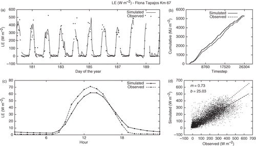
Figure 17. Results of NEE after hierarchical calibration. The graphs represent (a) sample of 10-day series data, (b) cumulative sum, (c) typical day and (d) scatter plot.
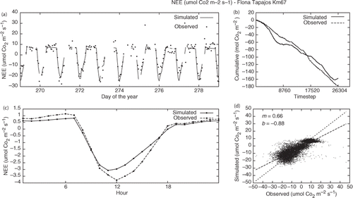
Figure 18. Results of LAI after hierarchical calibration. The graphs represent (a) a year of monthly data and (b) scatter plot.

shows hierarchically calibrated PARo. The adjustment for PARo hourly data was practically perfect, presenting an unbiased simulation () and with the linear regression coefficients m = 1.00 and b = 0.03 ().
presents hierarchically calibrated fAPAR. Observed and simulated data were well-adjusted. The linear regression coefficients were m = 0.77 and b = 0.19.
shows hierarchically calibrated Rn. Simulated Rn data had good adjustment to the observed Rn, with a linear regression line close to the 1:1 ratio. By observing the typical day graph () and the cumulative sum graph bias (), a little overestimation can be noticed for the simulated Rn night period, similar to the mono-objective calibration.
presents hierarchically calibrated u*. High values are underestimated while low values are overestimated, similar to mono-objective calibration results.
Hierarchically calibrated H results are presented in . An expressive bias between simulated and observed data is observed (), which is defined by overestimating fluxes throughout the day, in addition to a shift in the daily peak ().
displays hierarchically calibrated LE. The bias observed between simulated and observed LE is small, i.e. the cumulative sum curves are very close to each other. A small night time LE overestimate and a day time LE underestimate can be observed throughout the data series ().
presents hierarchically calibrated NEE. Simulated NEE was well-adjusted to observed, with a quite satisfactory adjustment for long-term analysis () and a reasonable daily behaviour (). shows an hour delay on day period NEE minimum value.
Simulated annual NPP was 1.017 kg-C m−2 year−1 and the correspondent field value was 1.055 kg-C m−2 year−1. Finally, presents hierarchically calibrated LAI. As in the mono-objective calibration, simulated and observed LAI data were well-adjusted, despite the bad linear regression result.
The obtained parameters’ values after hierarchical calibration are presented on , sorted by the hierarchical levels in which they were calibrated.
Table 5. Parameter values obtained in the hierarchical calibration procedure in the Tapajós National Forest km 67 site.
5. Discussion
The computer time for optimization depends mainly on the parameters of the GA (population size and number of generations) and the number of hierarchical levels. For one hierarchical level, the computational cost does not significantly differ between mono- and multi-objective optimizations, as the difference is only in the calculation of the objective functions, a minor cost. On the other hand, the optimization time increases with the number of hierarchical levels (see algorithm structure in ).
Individual results from hierarchical calibration tend to be worse than the ones from mono-objective. This is expected, since during mono-objective calibrations, each variable was exclusively optimized, disregarding all the others.
The goal of the hierarchical calibration is a global model calibration, optimizing all simulated variables in the best way possible. During the calibration, it is possible that the objective of a certain variable degrades when another variable is separately optimized and in a different hierarchical level of the calibration process.
The relative performance metric obtained was D = 0.801 (excluding NPP result from its calculation). Although there was a degradation of performance comparing to mono-objective calibration, the hierarchical procedure provides a more realistic model calibration, since all model-simulated variables are optimized to accurately simulate all the represented processes.
Regarding the turbulent fluxes in all calibrations done, the slope m in linear regression line is smaller than 1.0. This turbulent fluxes’ behaviour is related to the model difficulty in simulating turbulence for stable and unstable atmospheric conditions. Once the model overestimates low u* values and underestimates high u* values, such behaviour tends to repeat itself for the turbulent fluxes.
Generally, simulated variables presented good results after calibrated. The greatest bias is noticed on H, which is explained by the poor simulation for the night time fluxes. Even on the mono-objective calibration, the night period simulation for H was not properly adjusted. This night period H excess is certainly related to the night period Rn excess that, probably, responds to the Lin estimation methodology (Equation 6), in which the canopy emission temperature is assumed equivalent to air temperature. This simplification also affects H calculation, which is proportional to the temperature difference between canopy and air.
Other possible cause for H simulation deficiency could be uncertainties on field data measurement. A fundamental problem with eddy covariance system is that the energy budget usually is imprecise, with an error of 20% or even greater Citation42,Citation48. This violates the principle of conservation of energy, in which model construction is based.
6. Summary, conclusions and recommendations
This study developed an automatic multi-objective calibration system for the IBIS model and a general calibration methodology for LSEMs based on systems’ hierarchy. The multi-objective calibration system (Optis) relied on the NSGA-II multi-objective GA and allowed simultaneous calibration of the model for several statistics and many model outputs. The hierarchical calibration procedure was based on hierarchical temporal organization of natural systems, which is also reflected on the structure of the IBIS model. This methodology used the multi-objective calibration system to optimize processes occurring in different time scales.
Optis is an IBIS’ automatic calibration system that was developed to provide a more reliable and efficient optimization for model calibration, considering multiple objectives. In order to evaluate the multi-objective calibration performance, a relative calibration metric (D) was proposed to evaluate multi-objective calibrations in relation to mono-objective calibrations. This metric provides an evaluation that is independent of other errors embedded in the results, which are not due to the calibration method. At the multi-objective calibration test with multiple statistics, Optis performance was D = 0.925. At the multi-objective calibration test with multiple model outputs, Optis performance was also D = 0.925. This indicates that Optis is efficient for multi-objective calibration problem solving.
Finally, a hierarchical calibration procedure was proposed using Optis software. The hierarchical procedure was tested in Tapajós National Forest, an Amazon forest site. On this site, the hierarchical method granted nine objective functions optimizations, calibrating eight model outputs with a D index equal to 0.801. Despite the performance degradation loss in relation to mono-objective calibration, the hierarchical procedure provides a more realistic model calibration since every model output was optimized.
Based on this study, it is also possible to identify several works to be developed in the future:
| • | Statistics evaluation for model calibration specially combined in a multi-objective calibration. Optis allows several model calibrations with different statistics combined in multiple objectives. Hence, it may be possible to identify the fittest set of statistics or adjustment metrics for model calibration. | ||||
| • | Multi-objective calibration considering multiple sites, through Optis software use. Using a multi-site calibration, it may be possible to identify representative parameters’ values for an entire region. | ||||
| • | Multi-objective calibration considering remote sensing 2D data. As for multiple sites calibration, it may be possible to determine representative parameters values for an entire given region through remote sensing data. | ||||
Acknowledgements
The authors thank Dr Scott Saleska, University of Arizona, for the field data used in this study. CGV and CCSC were supported through CNPq fellowships.
References
- Sellers, PJ, Dickinson, RE, Randall, DA, Betts, AK, Hall, FG, Berry, JA, Collatz, GJ, Denning, AS, Mooney, HA, Nobre, CA, Sato, N, Field, CB, and Henderson-Sellers, A, 1997. Modeling the exchanges of energy, water, and carbon between continents and the atmosphere, Science 275 (5299) (1997), pp. 502–509.
- Pitman, AJ, 2003. The evolution of, and revolution in, land surface schemes designed for climate models, Int. J. Climatol. 23 (5) (2003), pp. 479–510.
- Costa, MH, Yanagi, SNM, Souza, PJO, Ribeiro, A, and Rocha, EJP, 2007. Climate change in Amazonia caused by soybean cropland expansion, as compared to caused by pastureland expansion, Geophys. Res. Lett. 34 (2007), p. L07706.
- Sampaio, G, Nobre, C, Costa, MH, Satyamurty, P, SoaresFilho, BS, and Cardoso, M, 2007. Regional climate change over eastern Amazonia caused by pasture and soybean cropland expansion, Geophys. Res. Lett. 34 (2007), p. L030612.
- M.C. Fu, F.W. Glover, and J. April, Simulation Optimization: A Review, New Developments, and Applications, in Proceedings of the 2005 Winter Simulation Conference, Orlando, FL, 4–7 December 2005, M. Kuhl, N. Steiger, F. Armstrong, and J. Joines, eds., Institute of Electrical and Electronics Engineers, Piscataway, NJ, 2005, pp. 83–95.
- Trudinger, CM, Raupach, MR, Rayner, PJ, Kattge, J, Liu, Q, Pak, B, Reichstein, M, Renzullo, L, Richardson, AD, Roxburgh, SH, Styles, J, Wang, YP, Briggs, P, Barrett, D, and Nikolova, S, 2007. OptIC project: An intercomparison of optimization techniques for parameter estimation in terrestrial biogeochemical models, J. Geophys. Res. 112 (G02027) (2007), p. 17.
- Nash, JE, and Sutcliffe, JV, 1970. River flow forecasting through conceptual models part i – A discussion of principles, J. Hydrol. 10 (1970), pp. 282–290.
- Johnston, PR, and Pilgrim, DH, 1976. Parameter optimization for watershed models, Water Resour. Res. 12 (3) (1976), pp. 477–486.
- Pickup, G, 1977. Testing the efficiency of algorithms and strategies for automatic calibration of rainfall-runoff models, Hydrol. Sci. Bull. 22 (2) (1977), pp. 257–274.
- Duan, QY, Gupta, VK, and Sorooshian, S, 1993. Shuffled complex evolution approach for effective and efficient global minimization, J. Optim. Theory Appl. 76 (3) (1993), pp. 501–521.
- Duan, Q, Sorooshian, S, and Gupta, V, 1992. Effective and efficient global optimization for conceptual rainfall-runoff models, Water Resour. Res. 28 (4) (1992), pp. 1015–1031.
- Gupta, HV, and Sorooshian, S, 1998. Toward improved calibration of hydrologic models: Multiple and noncommensurable metrics of information, Water Resour. Res. 34 (4) (1998), pp. 751–763.
- Yapo, PO, Gupta, HV, and Sorooshian, S, 1998. Multi-objective global optimization for hydrologic models, J. Hydrol. 204 (1998), pp. 83–97.
- Xia, Y, Pitman, AJ, Gupta, HV, Leplastrier, M, Henderson-Sellers, A, and Bastidas, LA, 2002. Calibrating a land surface model of varying complexity using multicriteria methods and the cabauw dataset, J. Hydromet. 3 (2002), pp. 181–194.
- Madsen, H, 2000. Automatic calibration of a conceptual rainfall-runoff model using multiple objectives, J. Hydrol. 235 (3) (2000), pp. 276–288.
- Madsen, H, 2003. Parameter estimation in distributed hydrological catchment modelling using automatic calibration with multiple objectives, Adv. Water Res. 26 (2) (2003), pp. 205–216.
- Vrugt, JA, Gupta, HV, Bastidas, LA, Bouten, W, and Sorooshian, S, 2003. Effective and efficient algorithm for multi-objective optimization of hydrologic models, Water Resour. Res. 39 (8) (2003), pp. SWC5.1–SWC5.19.
- Tang, Y, Reed, P, and Wagener, T, 2006. How effective and efficient are multi-objective evolutionary algorithms at hydrologic model calibration?, Hydrol. Earth Syst. Sci. 10 (2006), pp. 289–307.
- Bekele, EG, and Nicklow, JW, 2007. Multi-objective automatic calibration of SWAT using NSGA-II, J. Hydrol. 341 (2007), pp. 165–176.
- Foley, JA, Prentice, IC, Ramankutty, N, Levis, S, Pollard, D, Sitch, S, and Haxeltine, A, 1996. An integrated biosphere model of land surface processes, terrestrial carbon balance, and vegetation dynamics, Global Biogeochem. Cycles 10 (4) (1996), pp. 603–628.
- Morris, MD, 1991. Factorial sampling plans for preliminary computational experiments, Technometrics 33 (2) (1991), pp. 161–174.
- Deb, K, Pratap, A, Agarwal, S, and Meyarivan, T, 2002. A fast and elitist multi-objective genetic algorithm: NSGA-II, IEEE Trans. Evol. Comput. 6 (2) (2002), pp. 182–197.
- A. Saltelli, K. Chan, and E.M. Scott (eds.), Sensitivity Analysis, Wiley & Sons, Chichester, 2000.
- Saltelli, A, Ratto, M, Tarantola, S, and Campolongo, F, 2005. Sensitivity analysis for chemical models, Chem. Rev. 105 (7) (2005), pp. 2811–2827.
- Fox, DG, 1980. Judging air quality model performance, Bull. Am. Meteorol. Soc. 62 (1980), pp. 599–609.
- Willmott, CJ, 1981. On the validation of models, Phys. Geogr. 2 (2) (1981), pp. 184–194.
- Willmott, CJ, 1982. Some comments on the evaluation of model performance, Bull. Am. Meteorol. Soc. 63 (11) (1982), pp. 1309–1313.
- Willmott, CJ, Ackleson, SG, Davis, RE, Feddema, HJ, Klink, KM, Legates, DR, O’Donnell, J, and Rowe, CM, 1985. Statistics for the evaluation and comparison of models, J. Geophys. Res. 90 (C5) (1985), pp. 8995–9005.
- Willmott, CJ, and Matsuura, K, 2005. Advantages of the mean absolute error (MAE) over the root mean square error (RMSE) in assessing average model performance, Climate Res. 30 (2005), pp. 79–82.
- Legates, DR, and McCabe, G.J., 1999. Evaluating the use of “goodness-of-fit” metrics in hydrologic and hydroclimatic model validation, Water Resour. Res. 35 (1) (1999), pp. 233–241.
- Duan, Q, Schaake, J, Andréassian, V, Franks, S, Goteti, G, Gupta, HV, Gusev, YM, Habets, F, Hall, A, Hay, L, Hogue, T, Huang, M, Leavesley, G, Liang, X, Nasonova, ON, Noilhan, J, Oudin, L, Sorooshian, S, Wagener, T, and Wood, EF, 2006. Model parameter estimation experiment (MOPEX): An overview of science strategy and major results from the second and third workshops, J. Hydrol. 320 (2006), pp. 3–17.
- C.R. Reeves (ed.), Modern Heuristic Techniques for Combinatorial Problems, McGraw-Hill, New York, 1995.
- Jones, DF, Mirrazavi, SK, and Tamiz, M, 2002. Multi-objective meta-heuristics: An overview of the current state-of-the-art, Eur. J. Oper. Res. 137 (1) (2002), pp. 1–9.
- Goldberg, DE, 1989. Genetic Algorithms in Search, Optimization and Machine Learning. New York: Addison Wesley; 1989.
- Veldhuizen, DAV, and Lamont, GB, 2000. Multi-objective evolutionary algorithms: Analyzing the state-of-the-art, Evol. Comput. 8 (2) (2000), pp. 125–147.
- Zitzler, E, Deb, K, and Thiele, L, 2000. Comparison of multiobjective evolutionary algorithms: Empirical results, Evol. Comput. 8 (2) (2000), pp. 173–195.
- Saleska, SR, Miller, SD, Matross, DM, Goulden, ML, Wofsy, SC, da Rocha, HR, de Camargo, PB, Crill, P, Daube, BC, de Freitas, HC, Hutyra, L, Keller, M, Kirchhoff, V, Menton, M, WilliamMunger, J, Pyle, EH, Rice, AH, and Silva, H, 2003. Carbon in amazon forests: Unexpected seasonal fluxes and disturbance-induced losses, Science 302 (2003), pp. 1554–1557.
- M.C.A. Senna, Fração da radiação fotossinteticamente ativa absorvida pela floresta tropical amazônica: Uma comparação entre estimativas baseadas em modelagem, sensoriamento remoto e medições de campo, Ph.D. diss., Universidade Federal de Viçosa, 2004.
- Turner, MG, Dale, VH, and Gardner, RH, 1989. Predicting across scales: Theory development and testing, Landscape Ecol. 3 (3–4) (1989), pp. 245–252.
- Srinivas, N, and Deb, K, 1995. Multi-objective function optimization using nondominated sorting genetic algorithms, Evol. Comput. 2 (3) (1995), pp. 221–248.
- Praditwong, K, and Yao, X, How well do multi-objective evolutionary algorithms scale to large problems, CEC 2007. IEEE Congress on Evolutionary Computation, CEC 2007, Singapore, 25–28 September 2007, pp. 3959–3966.
- R.C. Purshouse and P.J. Fleming, Conflict, Harmony, and Independence: Relationships in Evolutionary Multi-criterion Optimization, in Proceedings of the EMO, Faro, Portugal, 8–11 April 2003, pp. 16–30.
- O’Neill, RV, 1988. "Hierarchy theory and global change". In: Rosswall, T., Woodmansee, R.G., and Risser, P.G., eds. SCOPE 35 – Scales and Global Change: Spatial and Temporal Variability in Biospheric and Geospheric Processes. New York: Wiley & Sons; 1988. pp. 29–45.
- Luan, J, Muetzelfeldt, RI, and Grace, J, 1996. Hierarchical approach to forest ecosystem simulation, Ecol. Model. 86 (1996), pp. 37–50.
- Maayar, ME, Chena, JM, and Price, DT, 2008. On the use of field measurements of energy fluxes to evaluate land surface models, Ecol. Model. 214 (2008), pp. 293–304.
- Wilson, K, Goldstein, A, Falge, E, Aubinet, M, Baldocchi, D, Berbigier, P, Bernhofer, C, Ceulemans, R, Dolman, H, Field, C, Grelle, A, Ibrom, A, Law, BE, Kowalski, A, Meyers, T, Moncrieff, J, Monson, R, Oechel, W, Tenhunen, J, Valentini, R, and Verma, S, 2002. Energy balance closure at fluxnet sites, Agric. For. Meteorol. 113 (2002), pp. 223–243.
- H.M.A. Imbuzeiro, Calibração do modelo IBIS na floresta amazônica usando múltiplos sítios, M.S. thesis, Universidade Federal de Viçosa, 2005.
- Costa, MH, Biajoli, MC, Sanches, L, Malhado, ACM, Hutyra, LR, Rocha, HR, Aguiar, RG, and Araújo, AC, 2010. Atmospheric versus vegetation controls of Amazonian tropical rain forest evapotranspiration: Are the wet and seasonally dry rain forests any different?, J. Geophys. Res. 115 (2010), p. G04021.
