Identification of friction heat generation in sliding bearing by temperature data

Abstract

In this article, the method of thermal diagnostics of friction is proposed for evaluating the friction power by temperature data. The method is based on the inverse boundary-value problem solving of heat exchange and applied to the sliding bearings with rotary and reciprocating rotary shaft motion. The simplified mathematical models of the thermal process in a radial sliding bearing and their bounds of applicability have been defined. The results of the computational experiments on investigating the temperature field in a bearing with and without regard to the shaft mobility have been presented. The authors have developed the algorithm of recovering the friction heat generation in a bearing by temperature data and showed it's efficiency for the thermal diagnostics of friction.

Keywords:

• temperature
• mathematical model
• heat generation
• friction
• inverse problem
• regularization

1. Introduction

The existing methods of the direct measurement of friction power require the use of special elastic elements. The arrangement of these elements in the friction units of the test and operating machinery is very complicated. As a result, it involves other magnitudes to be measured to determine the friction work consumed. In terms of accessibility temperature data are viewed as the most suitable as they do not require any complex and bulky equipment. Temperature is the most accessible for the direct measurement procedures including the most unfavourable cases. Temperature recording in the vicinity of the friction zone, construction of the mathematical heat model adequate to the heat exchange process in mating parts and the solution of the corresponding inverse boundary problem enable to recover the intensity of heat generated at friction. It is known that the prevailing part of the mechanical work of friction is transformed into heat, and the energy capacity of the other components of transformation is smaller in comparison with the heat generated 1, 2. Hence, we can assume that the found intensity of the friction heat generation approximately equals the friction power. Such an approach of determining the friction power by it's heat generation is called a method of thermal diagnostics of friction (MTDF).

Previously MTDF has been considered in the work 3 as applied to the sliding bearing made of a polymer antifriction material with a sufficiently high speed of shaft rotation that provided the uniform temperature distribution along the friction zone. This enabled, in it's turn, the rubbing elements to be considered as immovable while modelling the thermal process. In sliding bearings with reciprocating rotary motion (swinging movement) the elements were considered to be immovable at small amplitude and high frequency of shaft oscillations 4. It must be noted, however, that the earlier works devoted to the recovering the friction heat generation by temperature data disregarded the temperature dependence of materials on their properties that inevitably involved solving the non-linear inverse problem of heat exchange. In the given series of papers, we intend to set out MTDF for a sliding bearing with regard to the shaft mobility and the temperature dependence of materials on thermophysical properties as well as to show the efficiency of this method on computational and full-scale experiments. We have chosen a sliding bearing as the subject of our investigation due to it's adaptability for trying out a method of friction power recovery: it has a simple geometric shape and various specific characteristics of the contact interaction in friction units.

Though the process of recovering the intensity of heat generation implies the adequacy of the mathematical model to the real thermal process, we consider basically the two-dimensional model which serves as the ‘key’ one at constructing a more complete three-dimensional model and appropriate for developing methods of solving the boundary inverse heat exchange problem.

2. Thermal process modelling

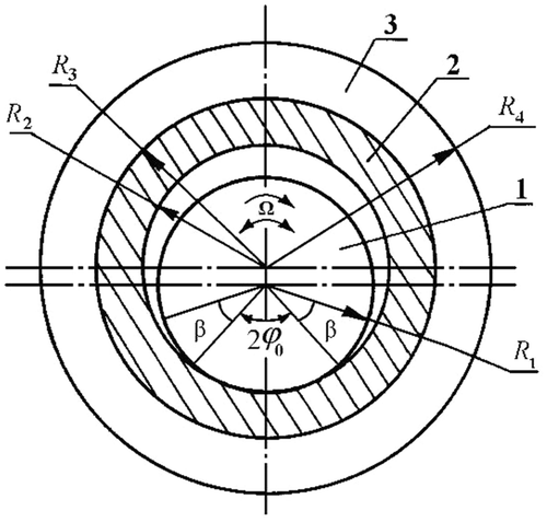
Let us consider a sliding bearing (Figure 1). The bush made of polymer composite material is tightly joined with the steel bearing race. The steel shaft makes rotary or reciprocating rotary motion with angular velocity . The temperature field calculation in non-lubricated sliding bearings without heat flow sharing coefficient has been presented in work 5. The latter implied the continuity of thermal contact with the shaft bush around the arc of the inner contour and used Fourier transform with finite bounds. In 6, temperature problem solution for sliding bearing was obtained by using finite element method. In the present work, we use method of finite differences 7 to define non-stationary temperature field in the sliding bearing.

Figure 1. Schematic of the bearing: 1 – shaft, 2 – bush and 3 – race.

The temperature distribution in the bush with the race is defined by the two-dimensional heat conduction equation: (1) – for the bush, for the race.

The temperature field in the bearing correlates with the temperature distribution in the shaft defined by the heat conduction equation with the convective term as regarding the shaft mobility: (2)

Assuming an intensive blowing in the bearing the ambient temperature inside and outside of the bearing is equal to and on the free surfaces of the shaft, bush and race the convective heat exchange conditions and heat exchange coefficients , , are specified by: (3) (4) (5)

In the centre of the shaft, the heat flow boundedness condition is specified by: (6)

In the contact zone, the lumped source of heat and the equality of temperatures are specified by: (7) (8)

Along the axis of symmetry of the design diagram, the periodicity conditions are fulfilled both for the bearing and the shaft: (9) (10)

The initial temperature distributions in the elements of the friction unit are considered to be equal and uniform (11)

For numerical solution of direct problems (1)–(11), we use method of splitting by spatial variables which involves step-by-step solution of one-dimensional equations by radial and angular variables. Accordingly, in solving the heat conduction equation for the shaft motion by an angular variable we use the monotone difference scheme 7, 8. Let us outline the numerical algorithm used.

First, let us introduce two space-time cylinders: – for bearing, and , – for shaft. In , let us define non-uniform meshes by radius and by angle, and a uniform mesh by time , , respectively, where , , , , , , , .

For Equations (1) and (2) in internal points we write the implicit locally-one-dimensional difference schemes of through calculation by radius and angle: (12) (13) (14) (15) where , – bearing and shaft temperatures in a point at time point t_k, , – intermediate values of temperatures at t = t_k + τ/2. Difference operators are defined by: (16) (17) where , – «differential Reynold's number» 7, , , , , , , , .

The system of Equations (12–15) supplemented by the difference analogues of the boundary conditions (3)–(10) are nonlinear, so their solutions are carried out by iterative method of progressive approximations 7. The whole system of equations is written in the form of a three-diagonal matrix system of equations. Let us show a generalized expression of this equation on an example of the differential system of equations (15): (18)

The iterative process for solution of nonlinear system of equations (18) is constructed as follows: (19) where – value of s + 1^st iteration of function . Relative to the difference scheme appears to be linear. The initial iteration is expressed by a value of desired function at the previous time layer – . The system (19) is solved by cyclic sweep method. Iterative process stops, the convergence condition being satisfied: . In all calculations we take ε = 0.001. The system (13) is solved by the same method. The systems of Equations (12) and (14) with corresponding difference analogues for boundary conditions are solved by iterative method involving opposite sweep methods by radial variables. The solutions match within conditions (7) and (8).

At thermal diagnostics of friction, the use of the mathematical model of the thermal process involving shaft mobility is not always efficient. There are rates of the shaft motion and oscillation amplitude that imply the shaft immobility and propose the use of simplified model. Such limiting kinematic parameters depend on the geometry of friction unit, thermophysical properties of materials, heat exchange conditions of free surfaces, etc. Therefore, for each particular sliding bearing one must investigate temperature fields at different sliding rates and then determine conditions for making one or another assumption.

Let us illustrate the conditions of applicability of the mathematical models involving shaft mobility. Take the sliding bearing with the following dimensions:  m,  m,  m,  m, . For numerical calculations parameters of meshes are set by: , ; ; , , . A time step is defined so that one period of oscillation or shaft rotation to be covered in 16 time steps. The given timing is based on numerous computation experiments as the most acceptable in terms of time and RAM saving. The latter is important in inverse problem solving which implies storage of the temperature value in bearing and shaft by space variables and time.

The bearing bush is made of a filled fluoroplastic with the dependences of thermophysical properties on temperature defined by: (Wm⁻¹°C⁻¹), (J m⁻³°C⁻¹). The material of the shaft and the race is steel:

The heat exchange coefficients are defined by: , (W m⁻²°C⁻¹). The initial temperature is T₀ = 20°C.

To show the dependence of shaft motion rate on bearing temperature field in calculations resulted below the function of the heat generation intensity is taken as equal to the both rotational and swinging motions of the shaft: (W). Thus, we see that the function depends only on the angular coordinate according to the parabolic law with maximum in the centre of the contact area.

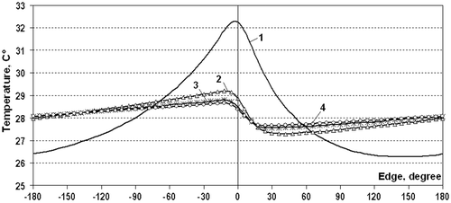
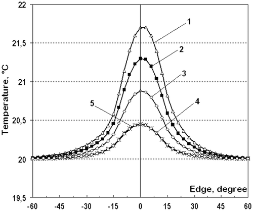
We calculated the nonstationary temperature fields in the bearing with regard to the rate of shaft rotation keeping a constant absolute value within the calculated time interval. The numerical results show that in course of time the increase in the shaft rotation rate results in the uniform temperature distribution along the shaft section. The maximum temperature value in the shaft is reached on the friction surface. Subsequently, this value slightly differs from the minimum one, and the higher is the rotation rate the less is the difference. The calculated temperature dependences of the shaft surface presented in Figure 2 show the dynamics of the tendency to the shaft temperature uniformity with the increase in the rotation rate.

Figure 2. Temperature distribution along the shaft surface at different rates of rotation at a time point t = 1 min: 1 – Ω = 3 rpm; 2 – 30 rpm; 3 – 48 rpm; 4 – 60 rpm.

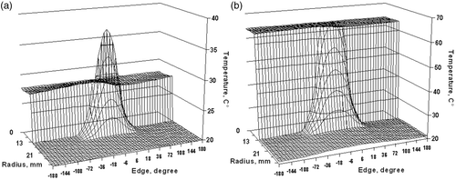
Figure 3 demonstrates the temperature fields in the shaft with sliding bearing at rotation rate at different time points. At rotation rate exceeding the given value, the temperature distribution can be considered to be uniform, as assumed previously 9. The shaft being considered as a one-dimensional bar has been proved valid by calculations. Still, while using such simplified model one should keep in mind that temperature uniformity on the shaft surface is achieved approximately in 7 min and this can result in the accuracy of recovering the function of heat generation intensity within this time interval.

Figure 3. Temperature fields in the shaft with the sliding bearing at a rate of the shaft rotation Ω = 48 rpm at different time points: (a) t = 1 min; (b) t = 7 min.

Let us analyse the dynamics of the sliding bearing temperature fields in case of swinging motion of the shaft. In this case, the conditions of the mathematical models applicability with regard to the shaft mobility are defined as reduced to the numerical experiments and analysis of calculations at different oscillation frequencies and amplitudes. Let us assume that a metal shaft makes swinging motions with some frequency and angular amplitude . The angular velocity of the shaft is . Suppose, the angle of the shaft contact with the bush during the tests remain constant. Since the shaft friction zone is larger than that in the bush, to verify the validity of the assumption concerning shaft immobility we must compare temperature distributions on the shaft surface obtained by the model both with and without regard to the shaft motion.

The calculated temperature distributions along the shaft surface (Figures 4 and 5) at swinging motion show that the decrease in oscillation amplitude and the increase in frequency result in a reduced influence of the convective term in Equation (2). As we see in Figure 5, at the amplitude of 3° and frequency of 2 Hz the results of calculations are practically the same as regarding so regardless to the convective term in Equation (2). Thus, at sufficiently small amplitudes and high oscillation frequencies it becomes possible to use the simplified model of the heat exchange in the sliding bearing, considering the shaft immobility assumption as described in earlier works 10,11.

Figure 4. Temperature distribution along the shaft surface at different swinging amplitudes and frequencies at a time point t = 1 s: 1 – β = 15°, ν = 2 Hz; 1′ – β = 15°, ν = 1 Hz; 2 – β = 9°, ν = 2 Hz; 2′ – β = 9°, ν = 1 Hz; 3 – without regard to the convective term.

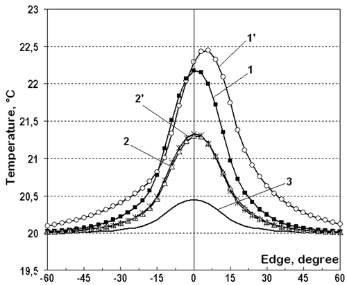
Figure 5. Temperature distribution along the shaft surface at different amplitudes and at the swinging frequency ν = 2 Hz at a time point t = 1 s: 1 – β = 12°; 2 – β = 9°; 3 – β = 6°; 4 – β = 3°; 5 – without regard to the convective term.

Therefore, for the successful thermal diagnostics of friction it is necessary to make preliminary analysis of the temperature fields for the different operating regimes of sliding bearings and to determine the kinematic conditions that imply the shaft mobility consideration.

3. Algorithm of determining the friction heat generation

Let us assume that kinematic conditions in the bearing require the shaft mobility in the mathematical thermal process model. The problem of determining the friction heat generation, i.e. the function , by temperature data relates to the inverse boundary problems. The latter are considered to be incorrect for they impose the solution instability to the temperature data errors. The given problems to be solved successfully one must use regularization methods 12. The methods for solving inverse problems of heat transfer are considered in works 13–18.

Let the temperature data in sliding bearing along the bush circle with the radius be defined by within the contact angle .

Let us now consider the extreme problem statement. A measure of deviation of calculated temperatures at known function approximation and measured is expressed by the squared residual (20)

Then, the inverse boundary problem is defined as follows. Functional (20) must be minimized at constraints in the form of combined equations (1–11). Function serves as a control function.

To solve the nonlinear problem of heat transfer, we use the method of iteration regularization based on the gradient methods of functional minimization theoretically appropriate for the linear statements. The formal application of the method for a nonlinear case requires the efficiency checking by numerical experiments with the use of model problems. Below we present the derivation of the basic relations required for realizing the method of iteration regularization 13.

The main problem of the gradient minimization comprises determining the gradient of the residual functional (20), i.e. finding the first Frechet derivative. Function is called the gradient of functional (20) if the functional increment can be defined by (21) where at at .

The efficient method of determining the gradient is the introduction of the conjugate boundary-value problem. Let the control be assigned with the increment , the temperatures and receiving the increments and , respectively. From the system of Equations (1–11) with controls and for the increments and , we obtain the equations (22) (23) (24) (25) (26) (27) (28) (29) (30) (31) (32)

Using the Lagrange method of multipliers and the stationary condition of the variational problem of minimizing functional (20), we obtain the conjugate problem relative to the unknowns for the bush with the race and for the shaft: (33) where (34) (35) (36) (37) (38) (39) (40) (41) (42) (43)

The solution of the conjugate problem depends on the difference of the direct problem solution, obtained at some approximation of the desired function , and the preset experimental temperature . Within invariable thermophysical characteristics, there are no other external factors in the system affecting the conjugate problem solution. Thus, the conjugate problem solution serves as the function which reflects the deviation of the calculated temperatures from the experimental ones.

Using the conjugate boundary-value problem, we obtain the formula for calculating the gradient of functional (20): (44)

Let us describe the algorithm for solving inverse boundary problem by using the conjugate gradients method. Suppose we are given an approximation of function of heat generation intensity . Finding of the next approximation can be expressed by the subsequent chain of passage from k-th iteration to (k + 1)-th iteration: where (45) (46)

The initial approximation is arbitrarily assigned.

is defined by the following algorithm:

1.	Determine the temperature fields of bearing and shaft , by known approximation and direct problem solution (1)–(11).
2.	Solve the conjugate boundary value problem (33)–(43) by substituting the obtained values of temperature; calculate the gradient of residual functional and the conjugate direction by formulas (44), (45).
3.	Solve the problem of increments of temperatures (22)–(32) by substituting instead of .
4.	Define the descent steps and subsequent approach by formulas (46).
5.	Check the implementation of iterative regularization condition by , where , – a function dispersion .
6.	If the iterative regularization condition is not satisfied, return to point 1 with the subsequent k value, otherwise iterative process stops and current value is taken as the desired solution .

Note that under known temperature distributions in bearing and shaft the conjugate problem (33)–(43) and the problem in increments (22)–(32) are considered to be linear. Numerically they are solved by differential schemes similar to those of the direct problem solution, but without using of the iterative method.

To test the efficiency of the algorithm proposed, we carried out numerical experiments with the model function of the heat generation intensity specified. Using the function given above we solved the direct problem; its precise solutions in the corresponding measuring points in the bush were taken as the ‘measured’ temperature data. Then, with the function being considered unknown, we solved the inverse problem of its recovery basing on the known ‘measured’ temperature data. In all numerical calculations listed below, the model function of heat generation intensity was taken as equal to the rotational and swinging motion of the shaft: , where , , at at at at at at at at at at at 8 at . This type of heat generation intensity function was selected to simulate the real process of friction in bearing which is normally characterized by quiet rapid change in values of friction power and subsequently of heat generation intensity due to the wear films tear-off and other reasons.

The temperature data are taken in 11 measurement points located in the bush at m within the contact angle with steps , where . Calculation time is s.

Speed of the shaft movement for swinging motion is defined by , where is oscillation amplitude, (Hz) is oscillation frequency; speed of shaft movement for the rotational motion is defined by rpm.

The numerical results for recovering the function with the precise ‘measured’ temperature data, presented in Figures 6 and 7, show that the accuracy of recovering grows with the increase of the iteration number. The latter proves the method to be resistant to computational errors. At reciprocating rotary motion of the shaft, the approximations of heat generation intensity function are determined by oscillations (Figure 6), their amplitude raising as they approach to the periphery of the contact zone and oscillations frequency coincides with the oscillations frequency of the shaft. This position depends on the oscillations of the ‘measured’ temperature values in time at corresponding points of measurement caused by release of points on shaft surface from friction zone, cooling and further contacting with bush. It is obvious that the shaft points contacting with the peripheral points of contact zone longer are outside of friction zone and the temperature oscillations amplitude is higher than those for the points close to the centre of the contact area. At recovering the heat generation intensity function oscillations remain regular, however, with the iteration number increase the approximate solution of the inverse problem becomes the precise one.

Figure 6. Comparison of the approximate solutions of the inverse problem with precise value of the model function of heat generation intensity for the reciprocating rotary motion of the shaft at ϕ = 0°, 9°, 12°: (1, 2, 3) – precise value; (1′, 2′, 3′) – approximation at 48 iteration; 1″, 2″, 3″ – approximation at 192 iteration. Т1, Т2, Т3 – «measured» temperature data at ϕ = 0°, 9°, 12°, respectively.

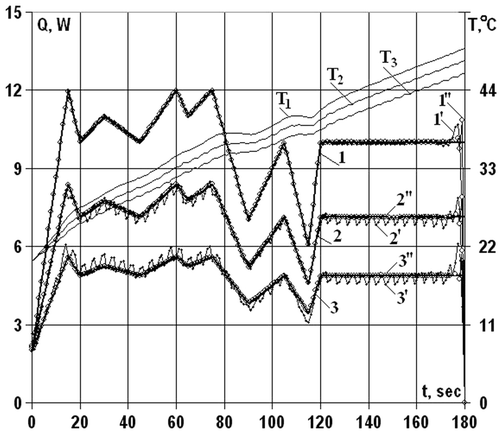
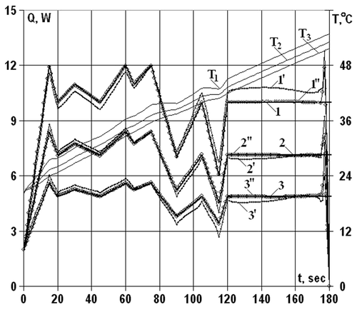
Figure 7. Comparison of the approximate solutions of the inverse problem with precise value of the model function of heat generation intensity for the rotary motion of the shaft at ϕ = 0°, 9°, 12°: (1, 2, 3) – precise value; (1′, 2′, 3′) – approximations at 37 iteration; 1″, 2″, 3″ – approximations at 139 iteration. Т1, Т2, Т3 – «measured» temperature data at ϕ = 0°, 9°, 12°, respectively.

Note that at the end of time interval the function of heat generation intensity is not recovered, which is associated with nulling of conjugate problem solution (33)–(43) for t = t_m. Practically, when recovering the heat generation intensity by temperature data, this negative effect can be decreased by omitting a number of, say 10, grid points at the end of the time interval.

Figures 8 and 9 show the results of solution of inverse problem by temperature data with errors. The errors in temperature data are simulated by: where – random variable distributed on the interval [−1, 1] according to the uniform law, – error level, – precise function. In this case, the function of heat generation intensity is recovered with greater error than while recovering with precise temperature data. The diagrams below show that the excessive increase of the iteration number causes the loss of the recovery accuracy. Therefore, the iterations stop and the functional residual value conforms with the temperature data inaccuracy level. The results of computational experiments revealed that the accuracy of recovering the heat generation intensity function is equivalent to the accuracy of the temperature data specified.

Figure 8. Comparison of precise value of the model function of heat generation intensity with approximate solutions of the inverse problem by temperature data with an error at ϕ = 0° for the reciprocating rotary motion of the shaft: 1 – precise value; 2 – approximations at 24 iteration; 3 – approximations at 38 iteration.

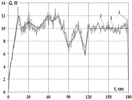
Figure 9. Comparison of precise value of the model function of heat generation intensity with approximate solutions of the inverse problem by temperature data with an error at ϕ = 0° for the rotary motion of the shaft: 1 – precise value; 2 – approximations at 21 iteration; 3 – approximations at 45 iteration.

The proposed algorithm of recovering the frictional heat generation function by temperature data can be applied to the thermal diagnostics of friction in the real friction units.

References

- Kuznetzov, VD, 1977. Physics of Cutting and Friction of Metals and Crystals: Selected Works. Moscow: Nauka; 1977.
- Kostetzky, BI, and Lynnik, YI, 1968. Energy balance at external friction of metals, Proc. USSR Ac. Sci. 183 (5) (1968), pp. 42–46.
- Starostin, NP, and Kondakov, AS, 1999. Boundary inverse problems of heat exchange for sliding bearing control and diagnostics, Inv. Prob. Eng. 7 (1999), pp. 565–580.
- Starostin, NP, and Kondakov, AS, 2002. Thermal diagnostics of friction in cylindrical connections: II. Computation experiments and generalization, J. Eng. Phys. Thermophys. 75 (5) (2002), pp. 1159–1164.
- Floquet, A, and Play, D, 1981. Contact temperature in dry bearings: Three dimensional theory and verification, ASME, J. Lubr. Technol. 103 (1981), pp. 243–252.
- Kennedy, FE, 1981. Surface temperature in sliding systems – A finite element analysis, ASME, J. Lubr. Technol. 103 (1981), pp. 90–96.
- Samarsky, AA, 1997. Theory of Difference Schemes. Moscow, Russia: Nauka; 1997.
- Samarsky, AA, and Vabyschevich, PN, 2003. Computational Heat Transfer. Moscow: Editorial URSS Publishers; 2003.
- Starostin, NP, Tikhonov, AG, Morov, VA, and Kondakov, AS, 1999. Calculation of Tribotechnical Parameters in Sliding Bearings. Yakutsk: YSC SB RAS Publishing; 1999.
- Starostin, NP, Kondakov, AS, and Vasilieva, MA, 2007. Thermal diagnostics of friction in self-lubricating radial slide bearings of swinging movement. Algorithm of determining the friction of heat generation power, J. Friction Wear. 29 (28) (2007), pp. 351–360.
- Starostin, NP, Kondakov, AS, and Vasil’eva, MA, 2010. Thermal diagnostics of friction in self-lubricating radial plain bearings of swinging movement. Part 2. Accounting for shaft mobility in the mathematical model, J. Friction Wear. 31 (6) (2010), pp. 449–452.
- Tikhonov, AN, and Arsenin, VY, 1977. Solution of ill-posed problems. Washington, DC: Winston & Sons; 1977.
- Alifanov, O, Artyukhin, E, and Rumyantsev, A, 1995. Extreme methods for solving ill-posed problems with applications to inverse heat transfer problems. New York: Begell House; 1995.
- Beck, JV, Blackwell, B, and St. Clair, CR, 1985. Inverse heat conduction: Ill-posed problems. New York: Wiley Interscience; 1985.
- Beck, JV, Blackwell, B, and Haji-Sheikh, A, 1996. Comparison of some inverse heat conduction methods using experimental data, Int. J. Heat Mass Transfer. 39 (17) (1996), pp. 3649–3657.
- Tillmann, AR, Borges, VL, Guimarães, G, Lima e Silva, ALF, Lima, SMM, and Silva, E, 2008. Identification of temperature-dependent thermal properties of solid materials, J. Braz. Soc. Mech. Sci. Eng. 30 (4) (2008), pp. 269–278.
- Frackowiak, A, Botkin, ND, Cialkowski, M, and Hoffmann, KH, 2010. A fitting algorithm for solving inverse problems of heat conduction, Int. J. Heat Mass Transfer. 53 (9–10) (2010), pp. 2123–2127.
- Pourgholi, R, and Rostamian, M, 2010. A numerical technique for solving IHCPs using Tikhonov regularization method, Appl. Math. Modelling. 34 (8) (2010), pp. 2102–2110.