Ritz–Galerkin method for solving an inverse heat conduction problem with a nonlinear source term via Bernstein multi-scaling functions and cubic B-spline functions

Abstract

Two types of basis functions are employed to find the approximate solution of the surface heat flux histories and temperature distribution in an inverse heat conduction problem (IHCP). The properties of Bernstein multi-scaling functions are first presented. These properties, together with Galerkin method, are then utilized to reduce the main problem to the solution of nonlinear algebraic equations. The approximation of the problem is based on the Ritz–Galerkin method. Also the B-spline scaling functions are used in the Ritz–Galerkin technique to solve the inverse problem. Both approximations provide greater flexibility in which initial and boundary conditions on rectangular bounded domains are imposed. To keep matters simple, the problem has been considered in one-dimensional case, however the techniques can be employed for two- and three-dimensional cases. Compared with other published methods, it has high accuracy in computations that leads to exact solutions in some cases. Some illustrative examples are included to demonstrate the validity and applicability of the two new techniques.

Keywords:

• Bernstein multi-scaling functions
• B-spline scaling functions
• Ritz–Galerkin method
• principal axis method
• inverse heat conduction problem
• surface heat flux

AMS Subject Classifications:

• 35K05
• 35K20
• 65M32
• 65M70

1. Introduction

In this work we consider the following inverse problem: (1) with the initial condition (2) and boundary conditions: (3) and extra specification (4) where F, f and g are considered as known functions while a(t) and A(x, t) are unknown functions. The function F(A(x, t)) is interpreted as a heat or material source, while in a chemical or biochemical application, it may be interpreted as a reaction term 1. Attention for studying parabolic inverse problems, specially in the last two decades, has been growing rapidly. The goal is to improve and develop more accurate methods, with both reliable analytical and numerical properties. Indeed, the aim is the determination of some unknown terms in the parabolic partial differential equations 2.

Physically speaking, the inverse heat conduction problem (IHCP) arises in the modelling and control of process with heat propagation in thermophysics and mechanics of continuous media. It occurs whenever surface temperatures and surface heat fluxes should be determined at inaccessible portions of the surface from the corresponding measurements at accessible parts 3. Determination of the unknown source term in a parabolic differential equation due to its variety of applications in the study of heat conduction processes, thermo-elasticity, chemical diffusion and control theory, has been discussed by several authors 4–20. More or less, all of them considered the initial and boundary conditions as given functions and their investigation focused on the identification of the unknown source term or thermophysical properties of the body. In these works, the insufficiency of the input information is reparable by some additional information on the surface, named by over specification data. However in this article, we propose to find a function (heat flux histories at x = 0) from the given measurements that are remote in some sense (see 1 and the related references therein). Meanwhile in this article we want to represent the new application of the Ritz–Galerkin method for finding the approximate solution of the IHCP using appropriate bases. This article is organized as follows.

As will be seen, we mention some necessary conditions for the existence and uniqueness of the direct problem in the next section. Then in Section 3, some properties of Bernstein polynomials are discussed. Section 4 is devoted to the function approximation using Bernstein multi-scaling functions (BMFs). Section 5 briefly introduces the Ritz–Galerkin method. In Section 6, we implement the problem with the Ritz–Galerkin method via BMFs. In Section 7, we resolve the problem using the B-spline scaling functions. Our numerical findings appear to demonstrate the validity, accuracy and applicability of the presented methods in Section 8. Section 9 consists of a brief summary.

2. Some backgrounds on the direct heat conduction problem

For a given function a(t), the parabolic problem (1.1)–(1.3) will be referred as a direct (or forward) problem that is well-posed. However, it is the fundamental difference between the direct and inverse problems, and the reader who merely wishes to become familiar with the most basic concepts of inverse problems need to know that there is a far difference between the direct and inverse problems in both approaches of their behaviours and solution procedures 21, but the central question to be answered in this section is to find conditions under which one can find the solution A(x, t) to the direct problem. The derivation of these properties can be found in 1. Let θ(x, t) denote the theta function defined by where K(x, t) is the free-space heat kernel moreover, we shall assume that the functions F, g, a have the following properties:

i.	f, g, a ∈ C[0, ∞),
ii.	The function F is piecewise differentiable on the set {A| − ∞ < A < ∞},
iii.	F is a bounded and uniformly continuous function in A. Furthermore, there exists a constant CF, subject to ∥F(A) − F(V)∥ ≤ CF∥A − V∥, where , and QT = {(x, t), 0 ≤ x ≤ 1, 0 ≤ t ≤ T}.

It is well known that the hypotheses (i)–(iii) are sufficient to imply the local existence of a solution to the problem (1.1)–(1.3), and if the local solution and its partial derivatives with respect to x satisfy a priori estimate, then the local solution may be extended to a global and unique solution on Q_T 1,2,22 as Now suppose that A = A(x, t; F, g, f, a) be the solution of the problem (1.1)–(1.3), then function p(t) = A(1, t; F, g, a) will be viewed as an output corresponding to the input g(t) in the presence of the heat flux a(t) = A_x(0, t). Now we state the following theorem that relates the interaction of a change Δa with the corresponding change Δp in the measured output p(t) which has been proven in 1.

Theorem 1

Suppose that the data functions g = g(t), F = F(A) and the heat flux terms q₁ and q₂ at x = 0 satisfy assumptions (i)–(iii). Let A_n = A(x, t; F, g, f, a_n) and p_n(t) = A_n(1, t), for n = 1, 2. Then for any τ ∈ [0, T], (5) where ξ(x, t) denotes a solution of the following suitable adjoint problem with input data ϑ(t): (6) Note that the problem (2.2) is backward in time, but is well posed 1; thus the solution is controlled by the inhomogeneous Neumann condition at x = 0, also it is easily seen that the properties of p(t) = A(1, t) can be found from assumptions on the inputs g(t) = A_x(1, t), a(t) = A_x(0, t). These properties expose conditions of compatibility on the p, g, a in an inverse problem associated with (1.1)–(1.4). These conditions, together with the properties of Theorem 1, lead to the definition of the class of admissible data 2 for the inverse problem considered in (1.1)–(1.4).

3. Properties of Bernstein polynomials

The Bernstein polynomials of mth-degree are defined on the interval [a, b] as 23 (7) where These m + 1, mth-order Bernstein polynomials form a basis on [a, b] (see 24 and the references therein). For convenience, we set B_i,m(x) = 0, if i < 0 or i > m. A recursive definition can also be used to generate the Bernstein polynomials over [a, b] so that the ith mth-degree Bernstein polynomials can be written as It can be readily shown that each of the Bernstein polynomials is positive and for all real x ∈ [a, b], It is easy to show that any given polynomial of degree m can be expanded in terms of these basis functions.

4. Properties of BMF

The BMFs ψ_i,n(t) = B_i,m(kt − n) have four arguments:

1.	Translation argument n = 0, 1, … , k − 1,
2.	Argument k > 1 which can assume any positive integer,
3.	m as the order of Bernstein polynomial on [0, 1],
4.	t, the normalized time.

They are defined on the interval [0, 1) as (8) Also the n-dimensional BMF are defined as (9) where X = (x₁, x₂, … , x_M), i = (i₁, i₂, … , i_M), n = (n₁, n₂, … , n_M), k_j as positive integer, m_j is the order of Bernstein polynomial B_i,m(x) and i_j = 0, 1, … , m_j, n_j = 0, 1, … , k_j − 1, j = 1, 2, … , M.

The functions {ψ_i,n(X)} form a basis for L²([0, 1]^M) (see 23 and the related references therein).

4.1. Function approximation

Suppose that H = L²[0, 1] and be the set of BMFs of mth-degree and and f be an arbitrary element in H. Since Y is a finite dimensional vector space, f has the unique best approximation out of Y such as y₀ ∈ Y, that is 25,26 where .

Accordingly where and c^T can be uniquely obtained by where ⟨φ, φ⟩ is the k(m + 1) × k(m + 1) dual operational matrix of φ, denoted by . Therefore we can write and In the following lemma we present an upper bound for the error approximation.

Lemma 1

Suppose that the function g : [0, 1) → ℝ is m + 1 times continuously differentiable, g ∈ C^m+1[t₀, t_f] and Y = Span{ψ_i,n(t) | i = 0, 1, … , m, n = 0, 1, … , k − 1}. If c^Tφ is the best approximation g out of Y, then the mean error bound is where

Proof

Let us consider the Taylor polynomial of order m for the function g on as for n = 0, 1, … , k − 1, for which (10) where Since c^Tφ is the best approximation g out of Y and y_n ∈ Y, therefore using (4.3) we have which results in the above bound 27.▪

Using the BMFs basis, we will have two degrees of freedom which increases the accuracy of the new method. One of these parameters is the argument k and another one is m that corresponds to the degree of Bernstein polynomials in every subinterval . As can be seen in the above lemma, the upper bound of the error depends on , which shows that the error reduces to zero very fast as m and k increase. This is one of the advantages of the Bernstein multi-scaling approximation.

5. The Ritz–Galerkin method

Consider the differential equation (11) multiplying it by any arbitrary weight function w(x) and integrating over the interval [a, b], one obtains (12) for any arbitrary w(x). Equations (5.1) and (5.2) are equivalent, because w(x) is any arbitrary function.

Now we approximate a trial solution u(x) to (5.1) of the form (13) Considering the residual the goal is to construct u(x) so that the integral of the residual vanishes for some choices of the weight functions. That is, u(x) will partially satisfy (5.2) in the sense that for some choices of w(x). One of the most important weighted residual methods was introduced by the Russian mathematician, Boris Grigoryevich Galerkin. Galerkin's method selects the weight functions in a special way: they are chosen from the basis functions, i.e. It is required that the following n equations hold true: To apply the method, we solve these n equations for the coefficients Suppose we wish to solve a boundary value problem over the interval [a,b] with the Ritz–Galerkin method, we select ϕ_i(x), i = 1, 2, … , m so that they satisfy the homogeneous form of the specified essential boundary conditions and ϕ₀ must satisfy the specified essential boundary conditions 25,28,29.

6. Solution of the inverse problem via Ritz–Galerkin method using BMFs

Consider the IHCP with a nonlinear source term introduced by Equations (1.1)–(1.4). Furthermore, suppose that a solution of the inverse problem (1.1)–(1.4) exists, and satisfies the condition ∣ A ∣ < C, for C > 0 and this implies that A(0, t) and A_x(0, t) are bounded piecewise continuous functions 1. Now put X = (x, t), M = 2, i = (i₁, i₂), n = (n₁, n₂). Our purpose is to implement the Ritz–Galerkin method for Equations (1.1)–(1.4) without imposing a(t) as a boundary condition. So, at first, we can find an approximation for A(x, t), like , that satisfies all the given initial and boundary conditions. Then, using we will obtain the approximate solution for a(t). Let (14) Substituting Equation (6.1) into Equation (1.1), we have 15 (15) with the initial condition (16) and the boundary condition (17) and the extra specification (18) Now a Ritz–Galerkin approximation to (6.2)–(6.5) is constructed as follows. The approximation is sought in the form of the truncated series (19) where and s(x) is the interpolating function as (20) This approximation satisfies the boundary and initial conditions (6.3)–(6.5). The expansion coefficients , are determined by the Galerkin equations: (21) i₁ = 0, 1, … , m₁, i₂ = 0, 1, … , m₂, n₁ = 0, 1, … , k₁ − 1, n₂ = 0, 1, … , k₂ − 1, where and denotes the inner product defined by Galerkin Equation (6.8), give a system of nonlinear equations which can be solved for the elements of using Newton's iteration method.

Remark 1

Newton's method with its modified form for which the global convergence can be proven for a large class of functions, yet are practical, but it is quite expensive since the Jacobian matrix must be computed at each iteration 30, especially when the number of equations is large. So, here we use this iteration method for solving the system of nonlinear equations (6.8) whenever the number of unknowns is small enough. We may assume that the necessary conditions for the convergence of Newton's method are satisfied. So starting with an initial guess , we stop the iteration and obtain the approximation if for some n and given ε, It is worthy to point out that our proposed technique presents the space-time approximation that fulfills all initial and boundary conditions. This results in requirements for only few spatial basis functions that approximate the problem with sufficient accuracy; so as will soon be apparent, this iteration method will be used in numerical examples.

6.1. Discussion on the regularization technique

The inverse problem is ill-posed or improperly posed in the sense of Hadamard. A problem is said to be ill-posed if one or more of these requirements are not satisfied, (a) existence, (b) uniqueness and (c) stability. Among these cases, the requirement of stability is the most important one. If the solution of a problem does not depend continuously on the data, then, in general, the computed solution has nothing to do with the exact solution 31. The numerical methods for solving discrete ill-posed problems have been presented in many papers. These methods are based on the so-called regularization techniques and the main goal of the regularization is to stabilize the problem and find a stable solution 32. The most common form of regularization is that of Tikhonov. Hence, one seeks a solution to the following optimization problem instead of (6.8): (22) where changes over , and λ ∈ R is called the regularization parameter, which fairly balances the perturbation error and the regularization error in the regularized solution. λ is usually as small as possible or even equal to zero for some configurations; however, care must be taken when noise is added into the additional boundary data 33. A reasonable choice of the regularization parameter is still a vital problem. Several approaches have been employed to find the suitable regularization parameter, it seems that the most widely used one is the L-curve criterion 34. However it is quite practical and we prefer to use this technique in solving linear systems; but here assuming the existence and uniqueness of the minimizer, we want to propose a useful method to solve (6.9), which in comparison to other direct methods is somewhat easy to implement and is low cost in computations. The method uses a type of a derivative-free algorithms 35 for a multi-variable problem named by principal axis method (PAM). To start the algorithm for a given Ξ-variable problem, we first need to have two apart conditions for each variable in order to define the norm of the search direction ρ_i, 1 ≤ i ≤ Ξ < ∞, then the algorithm takes a set of search directions ρ₁, … , ρ_Ξ, and a point σ₀ ∈ closure(ϖ)^Ξ, where (ϖ)^Ξ is the Ξ-dimensional cell restricted by the fixed primary conditions for the variables. Henceforth we employ the line search method 36,37 that controls the length of the direction by minimizing a one-dimensional function . Now suppose that σ_i be the point that minimizes along the direction ρ_i, from σ_i−1, then replace ρ_i with ρ_i+1. At the end, replace ρ_n with σ_n − σ₀. For more backgrounds about this method, we refer the reader to see 35,38,39. We emphasize that the regularization parameter λ will be most effective whenever the large number of basis functions leads to solving a large system of linear or nonlinear equations, especially if the noisy data have been added, employing the regularization technique is inevitable. Here the properties of the approximation given by (6.6) lead to a small system of equations in the sequel. Thus while noisy data have not been added, we consider λ = 0.

7. Implementation of the Ritz–Galerkin method using the cubic B-spline functions

The aim of this section is finding an approximate solution for problem (1.1)–(1.4) by compactly supported spline-scaling functions, constructed for the bounded interval [0, 1], because the domain of the problem is bounded 40. Let s and t be positive integers, the interval [α, β] is divided into t equal parts by a set of knots: while the left- and right-end knots have the multiplicity s 41. Cardinal B-spline functions of order s ≥ 2 for the knots sequence can be computed as and By considering the interval [α, β] ≡ [0, 1], at any level and unique solution j ∈ Z+, the discretization step is 2^−j, and this generates t = 2^j number of segments in [0, 1] with the knots sequence 41 Let j₀ be the level for which ; for each level j ≥ j₀, the scaling functions of order m can be defined as follows 41: The scaling functions occupy m segments, therefore the condition 2^j ≥ s must be satisfied in order to have at least one inner scaling function. The scaling functions used in this article are (cubic B-spline scaling functions), i.e. , with m = 4, j ≥ j₀ = 2. Note that the approximate solution for the unknown function A(η, ξ) given in (1.1) is defined over [a, b] × [c, d]. In order to expand this function in terms of the B-spline scaling functions, the finite intervals [a, b], [c, d] must be mapped to the interval [0, 1]. Therefore we employ the affine transformations 42: Henceforth reapplying the transform (6.1), we may deal with an equivalent form to the problem (6.2), with homogenous boundary conditions (6.4)–(6.5) and initial condition (6.3). Let be the proposed solution to problem (1.1)–(1.4), where are cubic B-spline functions (CBFs) and This approximation satisfies the boundary and initial conditions (6.3)–(6.5) too. The expansion coefficients, d_ij, are determined by the Galerkin equations: (23) where This process is similar to the previous technique, so at the end we can obtain the unknown coefficients d_ij, i, j = −3, … , 2^M − 1, in the content of system of nonlinear equations arising from the Galerkin equations (7.1), using Newton's iteration method. Moreover, all discussions on finding the regularization parameter in dealing with the large system of equations resulted from applying the BMF, can be extended to the case CBF.

8. Numerical examples

To get a better sense of the efficiency of the methods, let us employ the schemes presented in the current paper in solving some test problems. As is mentioned in the previous section, Newton's iteration method will be employed to solve the system of nonlinear equations. We implemented the proposed methods in the foregoing sections with Wolfram Mathematica 7.0 software in a personal computer and solved the final nonlinear equations. The initial guess for starting this process in all cases was considered as zero.

8.1. Example 1

Consider an IHCP given by Equations (1.1)–(1.4), as discussed in 1, subject to The exact solutions for this problem are We apply the method presented in this article with and solve problem (1.1)–(1.4) by both proposed bases. Using Equation (6.1), we have which together with Equation (6.7), s(x) = 0, and using Equations (6.8)–(7.1), we obtain Thus, from (6.1) and (6.6) we have , and from (1.3) we obtain , which agree with the exact solutions. We wish to investigate the stability of the presented methods in the context of this example by perturbing the additional specification data (1.4), as p^δ(t) = p(t) × [1 + δ(t, d)], where δ(t, d) is a random function of t uniformly distributed on (−d, d) and represents the level of relative error in the corresponding data set 11. We resolve the problem with the imposed random errors, {δ(t, 0.01), δ(t, 0.05)}, on the additional boundary data. Similar to the above statement, we first use (24) then using Equations (6.8)–(7.1), we obtain the following systems of linear algebraic equations: (25) for BMF, and (26) for CBF. Systems of linear algebraic equations, (8.2) and (8.3), can be represented by (27) where the vectors c, d denote the vectors of unknown constants and Q₁ and Q₂ are the square matrices of size 4 × 4 and 16 × 16, respectively. As already noted, we expect that the influence of perturbations can be seen significantly, whenever the calculations result in a large system of equations. Here the largest system can be found by using CBF, which consequently must solve the system Q₂d = z₂, where Q₂ is a 16 × 16 full matrix. 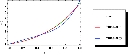Employing the Tikhonov regularization method leads to solving the new system , where is the transpose of matrix Q₂ and λ is the regularization parameter found by considering the corner of the L-curve, as suggested by Hansen 15. We take λ = 10⁻⁸ for δ(t, 0.01) and λ = 10⁻⁶ for δ(t, 0.05). As shown in Figure 1, the outcomes of the presented method (CBF) are in good adaptation to the exact solution and sensitive to artificial random errors. It is well known that the solution of heat flux at x = 0 for the final time t = T cannot be found accurately 33,43,44 if one uses the data (1.3) and (1.4). At first glance, without imposing noisy data we found the exact solutions. Nevertheless, we were interested in reporting our observations to find the approximations for a(t) = e^2t, from noisy data with error functions {δ(t, 0.01), δ(t, 0.05)}, (see Figure 1 and Table 1). As it can be seen, the errors increase as the time increases, especially it is more evident when noisy data comes from the error function δ(t, 0.05).

Figure 1. The approximated solutions of a(t) in the presence of the random errors for Example 8.1.

Table 1. Approximate solutions of a(t) with imposed error functions discussed in Example 8.1 by using CBF.

Heat flux	t = 0	t = 0.2	t = 0.4	t = 0.6	t = 0.8	t = 1
ã(t) for δ(t,0.01)	1.0000	1.4713	2.2133	3.3488	5.0076	7.3550
ã(t) for δ(t,0.05)	1.0000	1.7018	2.3084	3.0459	4.5255	7.7725
Exact values of a(t)	1.0000	1.4918	2.2255	3.3201	4.9530	7.3890

8.2. Example 2

Consider the problem with as the second example [1].

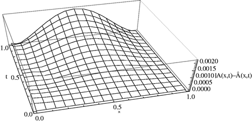
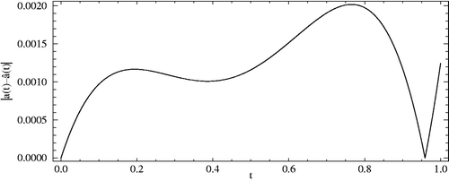
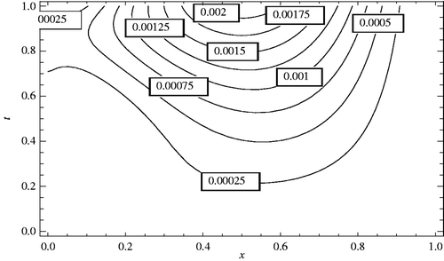
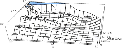
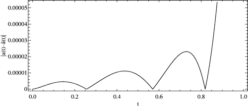
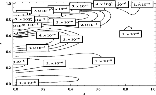
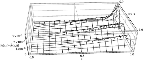
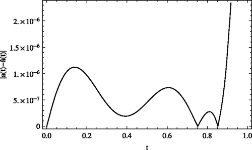
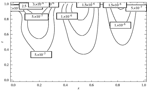
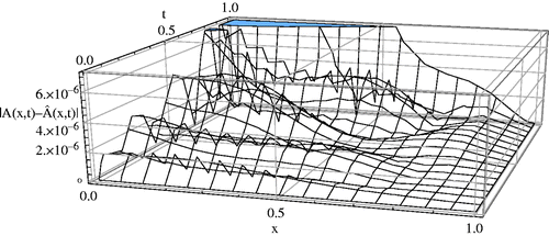
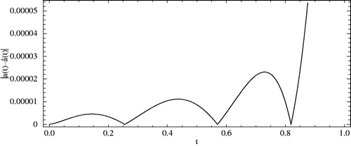
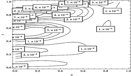
The exact solutions for this problem are In Figures 2–10, the absolute error between , , the Contour lines corresponding to the absolute errors attained by the Ritz–Galerkin method when and m₁ = m₂ = 5, are plotted. We solved all nonlinear systems using Newton's iteration method where the convenient stopping criterion was fixed on ε = 10⁻⁶. Noting Figures 2–10 along with Table 2, it can be seen that the numerical solution converges to the exact solution, as the number of basis increases. Again using this procedure for the CBF, we obtain the same result. Moreover, in Figures 11–13, the absolute errors between , and the Contour lines related to this absolute error utilizing the CBF are plotted for more comparisons. As already mentioned, noisy data should be involved to the overposed data (1.4), and then fluctuation of the heat flux must be reported to represent the numerical stability of the methods. Thus, similar to previous example, we applied the random errors, but this time the error function was set as {δ(t, 0.01)} only and handled both the proposed methods. Preferably the largest systems of equations were considered, which resulted from using BMF and CBF, when m₁ = m₂ = 3, m₁ = m₂ = 5 and i, j = −3, … , 0, respectively. It should be noted that for solving the latter problems, the optimization problem (6.9) was considered. Reciprocally, the main task was to focus on the PAM to find the minimizer of the problems. Two distinct starting conditions were chosen as {0, 2} for each variable. The results are depicted in Figures 14–16 and Tables 3–5. Reflection of these results has significant implications to the basic concepts of the inverse problems, particularly to IHCP. First, results highlight that the regularization technique plays an important role in presenting the real solution of severely ill-posed problems, as we can see that Newton's method gives answers which are different from exact solutions. Second, the logical continuity between the regularized solution and the noisy data is evident, which indicates the stability of the presented methods 11. Finally, we can observe that as time increases, the errors increase and it causes to some drawbacks for recovering the value of heat flux at t = T, accurately 43. So our findings confirm this fact and are in agreement with the results in 33,44. As the last point, we should underline that the PAM applied as a classical technique is efficient in terms of convergence rate and even usable to solving functions where symbolic derivatives are not available. But in order to be assured of meaningful solutions, we resolved the optimization problem (6.9) using the nonlinear conjugate gradient method 45 and found the same results in the whole cases.

Figure 2. The absolute error between when m₁ = m₂ = 1 for Example 8.2.

Figure 3. The absolute error between when m₁ = m₂ = 1 for Example 8.2.

Figure 4. Contour lines corresponding to Figure 2.

Figure 5. The absolute error between when m₁ = m₂ = 3 for Example 8.2.

Figure 6. The absolute error between when m₁ = m₂ = 3 for Example 8.2.

Figure 7. Contour lines corresponding to Figure 5.

Figure 8. The absolute error between when m₁ = m₂ = 5 for Example 8.2.

Figure 9. The absolute error between when m₁ = m₂ = 5 for Example 8.2.

Figure 10. Contour lines corresponding to Figure 8.

Figure 11. The absolute error between when i, j = −3, −2, −1, 0 for Example 8.2.

Figure 12. The absolute error between when i, j = −3, −2, −1, 0 for Example 8.2.

Figure 13. Contour lines corresponding to Figure 11.

Figure 14. Dash: The regularized solution of a(t) in the presence of the random function δ(t, 0.01) using BMF with m₁ = m₂ = 3, Thick line: Exact solution, Dot: Solution without regularization, related to Example 8.2.

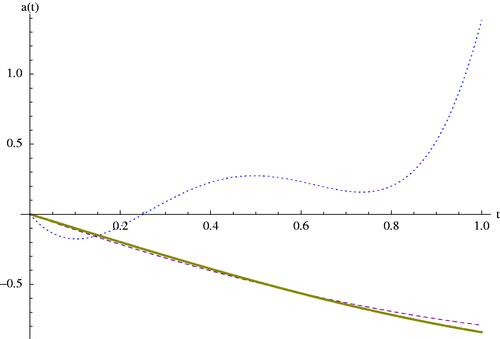
Figure 15. Dash: The regularized solution of a(t) in the presence of the random function δ(t, 0.01) using BMF with m₁ = m₂ = 5, Thick line: Exact solution, Dot: Solution without regularization, related to Example 8.2.

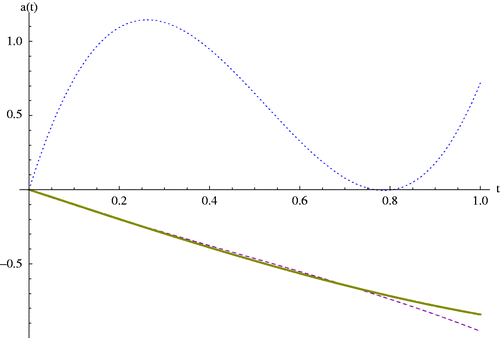
Figure 16. Dash: The regularized solution of a(t) in the presence of the random function δ(t, 0.01) using CBF with i, j = −3, … , 0, Thick line: Exact solution, Dot: Solution without regularization, related to Example 8.2.

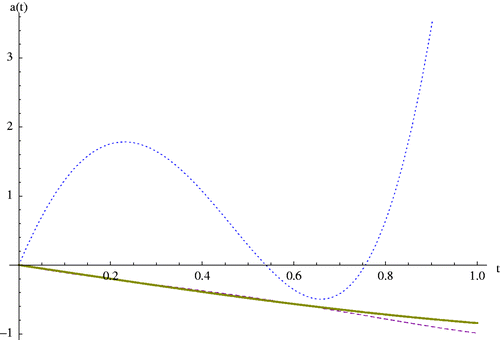
Table 2. Norm 2 of coefficient vectors c discussed in Example 8.2 attained by BMF.

Number of basis	m1 = m2 = 1	m1 = m2 = 3	m1 = m2 = 5
∥c∥2	0.3579	0.3593	0.3592

Table 3. Approximated solution of heat flux in the presence of random function δ(t, 0.01) discussed in Example 8.2, attained by PAM.

Time	(BMF), m1 = m2 = 3	(BMF), m1 = m2 = 5	(CBF), i,j = − 3,…,0	Exact
0.000	0.0000	0.0000	0.0000	0.0000
0.100	−0.1109	−0.1019	−0.1117	−0.0998
0.200	−0.2151	−0.1975	−0.2033	−0.1986
0.300	−0.3124	−0.2886	−0.2869	−0.2955
0.400	−0.4028	−0.3768	−0.3714	−0.3894
0.500	−0.4862	−0.4639	−0.4624	−0.4794
0.600	−0.5625	−0.5518	−0.5623	−0.5646
0.700	−0.6314	−0.6427	−0.6703	−0.6442
0.800	−0.6927	−0.7385	−0.7825	−0.7173
0.900	−0.7461	−0.8415	−0.8917	−0.7833
1.000	−0.7914	−0.9540	−0.9873	−0.8414

Table 4. Solution of heat flux in the presence of random function δ(t, 0.01) discussed in Example 8.2, without employing the regularization technique.

Time	(BMF), m1 = m2 = 3	(BMF), m1 = m2 = 5	(CBF), i,j = − 3, … , 0	Exact
0.000	0.0000	0.0000	0.0000	0.0000
0.100	−0.1757	0.7499	1.231	−0.0998
0.200	−0.0861	1.0940	1.7560	−0.1986
0.300	0.0882	1.1280	1.6474	−0.2955
0.400	0.2280	0.9478	1.0715	−0.3894
0.500	0.2751	0.6491	0.2867	−0.4794
0.600	0.2329	0.3275	−0.3567	−0.5646
0.700	0.1660	0.0784	−0.4162	−0.6442
0.800	0.2003	−0.0027	0.6429	−0.7173
0.900	0.5233	0.1792	3.4480	−0.7833
1.000	1.3836	0.7196	8.7182	−0.8414

Table 5. Values of regularization parameter λ in the presence of random function δ(t, 0.01) discussed in Example 8.2, attained by PAM.

Method	(BMF), m1 = m2 = 3	(BMF), m1 = m2 = 5	(CBF), i, j = − 3, … , 0
λ	9.2727 × 10^−8	7.3273 × 10^−8	4.165 × 10^−7

9. Conclusion and results

In this study two numerical procedures based upon the Bernstein multi-scaling approximation and the cubic B-spline scaling functions for solving the IHCP with a nonlinear source term are presented. The key to these methods is to utilize the features of the Bernstein and cubic B-spline scaling functions along with Galerkin's method to reduce the main problem to the solution of nonlinear algebraic equations. The new techniques are applied to solve two test problems and the resulting solutions are in good agreement with the known exact solutions. The procedures are applicable to nonlinear problems and to problems involving rectangular bounded domains. However, for the sake of simplicity, we only considered the one-dimensional case with standard initial and boundary conditions, but it can be extended to multi-dimensional cases with even nonclassic boundary conditions and it will be the future work of the authors. Numerical solutions are obtained efficiently and the stability is maintained for randomly perturbed data. From the practical point of view, both Bernstein polynomials and CBFs have great and valuable applications, however if one aims to approximate a discontinuous function, setting k > 1 (Section 4), can find a partitioned stiffness matrix where some of its blocks are zero. So in comparison to the same resulted matrix from the CBFs, if both matrices have the same dimension, then the first one is neater, so it may reduce the amount of computations. But here we believe that both BMF and CBF produce the same results while we are not encountered in evaluating some unknown discontinuous terms or leading coefficients, however both the proposed techniques lead to full stiffness matrices, but we should put in consideration that properties of the Ritz–Galerkin method compensate this drawback. Thus, the methods appear to be applicable to any formulation of this type of IHCPs.

Acknowledgements

We would like to thank the three referees for their valuable comments and helpful suggestions to improve the earlier version of this article.

References

- Shidfar, A, Caramali, GR, and Damirchi, J, 2006. An inverse heat conduction problem with a nonlinear source term, Nonlinear Anal. 65 (2006), pp. 615–621.
- Cannon, JR, and DuChateau, P, 1998. Structural identification of a term in a heat equation, Inverse Probl. 14 (1998), pp. 535–551.
- Hon, YC, and Wei, T, 2004. A fundamental solution method for inverse heat conduction problem, Eng. Anal. Bound. Elem. 28 (2004), pp. 489–495.
- Berres, S, , Identification of piecewise linear diffusion function in convection–diffusion equation with overspecified boundary, AIP Conf. Proc. 1048 (2008), pp. 76–79.
- Cannon, JR, and Dunninger, DR, 1970. Determination of an unknown forcing function in a hyperbolic equation from overspecified data, Ann. Mat. Pure Appl. 85 (4) (1970), pp. 49–62.
- Cannon, JR, and DuChateau, P, 1980. An inverse problem for determination an unknown source term in a heat equation, J. Math. Appl. 75 (2) (1980), pp. 465–485.
- Dehghan, M, 2001. An inverse problem of finding a source parameter in a semilinear parabolic equation, Appl. Math. Model. 25 (2001), pp. 743–754.
- Dehghan, M, 2003. Finding a control parameter in one-dimensional parabolic equations, Appl. Math. Comput. 135 (2003), pp. 491–503.
- Dehghan, M, 2005. Parameter determination in a partial differential equation from the overspecified data, Math. Comput. Model. 41 (23) (2005), pp. 196–213.
- Dehghan, M, and Shakeri, F, 2009. Method of lines solutions of the parabolic inverse problem with an overspecification at a point, Numerical Algorithms 50 (2009), pp. 417–437.
- Fatullayev, AG, and Cula, S, 2009. An iterative procedure for determining an unknown spacewise-dependent coefficient in a parabolic equation, Appl. Math. Lett. 22 (2009), pp. 1033–1037.
- Johansson, BT, and Lesnic, D, 2007. A variational method for identifying a spacewise-dependent heat source, IMA J. Appl. Math. 72 (2007), pp. 748–760.
- Johansson, BT, and Lesnic, D, 2008. A procedure for determining a spacewise dependent heat source and the initial temperature, Appl. Anal. 87 (2008), pp. 265–276.
- Mohebbi, A, and Dehghan, M, 2010. High-order scheme for determination of a control parameter in an inverse problem from the overspecified data, Comput. Phys. Comm. 181 (2010), pp. 1947–1954.
- Rashedi, K, and Yousefi, SA, 2011. Ritz–Galerkin method for solving a class of inverse problems in the parabolic equations, Int. J. Nonlinear Sci. 12 (2011), pp. 498–502.
- Saadatmandi, A, and Dehghan, M, 2010. Computation of two time-dependent coefficients in a parabolic partial differential equation subject to additional specifications, Int. J. Comput. Math. 87 (2010), pp. 997–1008.
- Slodicka, M, Lesnic, D, and Onyango, TTM, 2010. Determination of a time-dependent heat transfer coefficient in a nonlinear inverse heat conduction problem, Inverse Probl. Sci. Eng. 18 (2010), pp. 65–81.
- Trucu, D, Ingham, DB, and Lesnic, D, 2009. An inverse coefficient identification problem for the bio-heat equation, Inverse Probl. Sci. Eng. 17 (2009), pp. 65–83.
- Yousefi, SA, 2009. Finding a control parameter in a one-dimensional parabolic inverse problem by using the Bernstein Galerkin method, Inverse Probl. Sci. Eng. 17 (2009), pp. 821–828.
- Yousefi, SA, and Dehghan, M, 2009. Legendre multiscaling functions for solving the one-dimensional parabolic inverse problem, Numer. Methods Partial Diff. Eqns. 25 (2009), pp. 1502–1510.
- Lakestani, M, and Dehghan, M, 2010. The use of Chebyshev cardinal functions for the solution of a partial differential equation with an unknown time-dependent coefficient subject to an extra measurement, J. Comput. Appl. Math. 235 (2010), pp. 669–678.
- Cannon, JR, 1984. The One-dimensional Heat Equation. Reading, MA: Addison-Wesley; 1984.
- Idrees Bhatti, M, and Bracken, P, 2007. Solution of differential equations in a Bernstein polynomials basis, J. Comput. Appl. Math. 205 (2007), pp. 272–280.
- Rivlin, TJ, 1969. An Introduction to the Approximation of the Functions. New York: Dover; 1969.
- Yousefi, SA, Barikbin, Z, and Dehghan, M, 2012. Ritz–Galerkin method with Bernstein polynomial basis for finding the product solution form of heat equation with non-classic boundary conditions, Int. J. Numer. Methods Heat Fluid Flow 22 (1) (2012), pp. 39–48.
- Yousefi, SA, Behroozifar, M, and Dehghan, M, 2011. The operational matrices of Bernstein polynomials for solving the parabolic equation subject to specification of the mass, J. Comput. Appl. Math. 235 (2011), pp. 5272–5283.
- Yousefi, SA, Behroozifar, M, and Dehghan, M, 2012. Numerical solution of the nonlinear age-structured population models by using the operational matrices of Bernstein polynomials, Appl. Math Model. 36 (2012), pp. 945–963.
- Yousefi, SA, Barikbin, Z, and Behroozifar, M, 2010. Bernstein Ritz–Galerkin method for solving the damped generalized regularized long-wave (DGRLW) equation, Int. J. Nonlinear Sci. 9 (2010), pp. 151–158.
- Yousefi, SA, Barikbin, Z, and Dehghan, M, 2010. Bernstein–Ritz–Galerkin method for solving an initial-boundary value problem that combines Neumann and integral condition for the wave equation, Numer. Methods Partial Diff. Eqns. 26 (2010), pp. 1236–1246.
- Stoer, J, and Bulirsch, R, 1980. Introduction to Numerical Analysis. New York: Springer-Verlag; 1980.
- Kirsch, A, 1999. An Introduction to the Mathematical Theory of Inverse Problem. New York: Springer; 1999.
- Krawczyk-Stando, D, and Rudnicki, M, 2007. Regularization parameter selection in discrete ill-posed problems-the use of the U-curve, Int. J. Appl. Math. Comput. Sci. 17 (2) (2007), pp. 157–164.
- Johansson, BT, Lesnic, D, and Reeve, T, 2011. Numerical approximation of the one-dimensional inverse Cauchy–Stefan problem using a method of fundamental solutions, Inverse Probl. Sci. Eng. 19 (2011), pp. 659–677.
- Hansen, PC, 1992. Analysis of discrete ill-posed problems by means of the L-curve, SIAM Rev. 34 (1992), pp. 561–580.
- Brent, RP, 2002. Algorithms for Minimization Without Derivatives. Mineola, NY: Dover; 2002.
- More, JJ, and Thuente, DJ, 1994. Line search algorithms with fauranteed sufficient decrease, ACM T. Math. Software. 20 (3) (1994), pp. 286–307.
- More, JJ, and Weight, SJ, 1993. Optimization Software Guide. Philadelphia: SIAM; 1993.
- Dennis, JE, and Schnabel, RB, 1996. Numerical Methods for Unconstrained Optimization. Philadelphia: SIAM; 1996.
- Rheinboldt, WC, 1998. Methods for Solving Systems of Nonlinear Equations. Philadelphia: SIAM; 1998.
- Lakestani, M, and Dehghan, M, 2009. Numerical solution of Fokker–Plank equation using the cubic B-spline scaling functions, Numer. Methods Partial Diff. Eqns. 25 (2009), pp. 418–429.
- Nevels, RD, Goswami, JC, and Tehrani, H, 1997. Semiorthogonal wavelets basis sets for solving integral equations, IEEE Trans. Antennas. Propagation 45 (1997), pp. 1332–1339.
- Shamsi, M, and Dehghan, M, 2007. Recovering a time-dependent coefficient in a parabolic equation from overspecified boundary data using the pseudospectral Legendre method, Numer. Methods Partial Diff. Eqns. 23 (2007), pp. 196–210.
- Elden, L, 1983. "The numerical solution of a non-characteristic Cauchy problem for a parabolic equation". In: Deuflhard, P, and Hairer, E, eds. Numerical Treatment of Inverse Problems in Differential and Integral Equations. Basel: Birkhauser; 1983. pp. 246–268.
- Johansson, BT, Lesnic, D, and Reeve, T, 2011. A method of fundamental solutions for the one-dimensional inverse Stefan problem, Appl. Math. Model. 35 (2011), pp. 4367–4378.
- Adams, L, and Nazareth, JL, 1996. Linear and Nonlinear Conjugate Gradient-related Methods. Philadelphia: SIAM; 1996.