Drift reconstruction from first passage time data using the Levenberg–Marquardt method

Abstract

In this paper, we consider the problem of recovering the drift function of a Brownian motion from its distribution of first passage times, given a fixed starting position. Our approach uses the backward Kolmogorov equation for the probability density function (pdf) of first passage times. By taking Laplace transforms, we reduce the problem to calculating the coefficient function in a second-order ordinary differential equation (ODE). The inverse problem effectively amounts to finding the convection coefficient of the ODE, given the transformed pdf for positive values of the Laplace variable. Our first contribution is to find series solutions to the forward problem and show that the associated operator for the linearized inverse problem is compact. Our second contribution is numerical: for low noise levels, we reconstruct simple drift functions by applying Tikhonov regularization and performing a Newton iteration (Levenberg–Marquardt method). For larger noise, our solution displays large oscillations about the true drift.

Keywords:

• random walk
• first passage times
• drift reconstruction
• force spectroscopy

Introduction

In this paper, we shall be concerned with finding the drift function of a Brownian process with constant diffusion coefficient, given the first passage time distribution (FPTD). Consider a particle that undergoes a random walk, $Y(t)$, parametrised by a drift function $U(Y)$ and a constant diffusivity on the interval $[0,1]$. Let the starting position be $Y(t=0)\equiv x$ where $0\le x<1$. The particle cannot cross $Y=0$ where there is a ‘reflecting’ boundary condition. When the value of $Y$ first reaches 1, the time is recorded. Upon repeating the process many times, always starting at the same position $x$, one obtains a distribution of first passage times. From this data, can one infer the drift function $U$?

We can get some intuition for this problem by considering the governing stochastic differential equation (SDE) explicitly,(1) $$\begin{array}{c}\hfill \text{d}Y(t)=U(Y(t))\text{d}t+\sqrt{2D}\text{d}W(t),\end{array}$$(1) where $Y\in \mathbb{R}$, $\text{d}W$ is the Wiener measure and $D$ is a constant diffusivity. In the case where $D\to 0$, we have the deterministic equation $\stackrel{·}{Y}=U(Y)$. If the drift is always positive, the first passage time or exit time $T_e$ is given by(2) $$\begin{array}{c}\hfill T_e={\int }_x^1\frac{{\mathit{dx}}^{\prime }}{U(x^{\prime })},\end{array}$$(2) and it is clear in this limit that from a single exit time, no pointwise information about $U$ can be gained: there are many functions $U(·)$ that satisfy (2(2) $$\begin{array}{c}\hfill T_e={\int }_x^1\frac{{\mathit{dx}}^{\prime }}{U(x^{\prime })},\end{array}$$(2) ) for a given $T_e$. If $D>0$, we have a distribution of first passage times instead of a single time; now there is at least a possibility that some more information about $U$ can be extracted.

The study of these types of exit time problems is motivated by experiments that involve the dissociation of receptor–ligand complexes.[1–4] In these experiments, the force on a complex is increased until rupture occurs at a critical force. The experiment is repeated many times to obtain a distribution of rupture forces; thermal fluctuations ensure the rupture does not occur at a single fixed force. The objective of these experiments is to infer some quantitative features of the bond such as its dissociation constant. In the theoretical modelling of such systems, the rupture of the complex is assumed to proceed along a one-dimensional bond coordinate. Specifically, the problem can be treated as escape from a potential well.[5–8] Time dependent potentials (corresponding to the explicit application of a force ramp or a time-dependent drift function) can also be included.[9] However, in this paper, we restrict ourselves to time independent potentials wells/drift functions.

One framework for approaching these stochastic inverse problems is to use the (deterministic) backward partial differential equation for the FPTD.[10] After taking Laplace transforms, the problem amounts to calculating the coefficient function in a second-order differential equation. Mathematically, these types of problems have a long history, dating back to Borg.[11] The aim of inverse Sturm–Liouville problems is to reconstruct the coefficient in the differential operator from its eigenvalues. Although spectra can be generated from the exit time distribution in certain cases, in our problem, we do not have direct access to eigenvalues. Nevertheless, a large body of work exists that discusses both analytic [12, 13] and numerical methods [14, 15] for coefficient reconstruction from its eigenvalues.

There are also several variations of the stochastic inverse problem where the quantity to be reconstructed and/or given data are different. We mention here a few recent theoretical and experimental studies. The assumption of constant $D$ in Equation (1(1) $$\begin{array}{c}\hfill \text{d}Y(t)=U(Y(t))\text{d}t+\sqrt{2D}\text{d}W(t),\end{array}$$(1) ) can be relaxed and could be inferred along with $U$ – this case was studied in [16]. One could also infer the drift and diffusivity from knowledge of particle positions. Förster resonance techniques applied to ensembles of folding proteins [17] give time snapshots of the probability distribution of $Y$ from which it may be possible to infer $U$. In [18], functional forms of 2D drifts and a constant diffusivity were inferred from measurements of particle positions using Bayesian techniques.

In this paper, we we propose a Levenberg–Marquardt method to recover the drift function from the FPTD. The method is based on repeatedly solving a first-kind linear integral equation using regularization techniques. Unlike previous work, [19] we do not a priori assume that the drift function can be decomposed into a pre-defined set of basis functions. At each stage, the regularization parameter is calculated using a method similar to Morozov’s discrepancy principle.

In Section 2, we derive the backward Kolmogorov equation that governs the exit time distribution in terms of a spatially dependent drift function. This equation defines a map from the drift to the exit time distribution. We also state the forward and inverse problems. In Section 3, we discuss our algorithm generally and prove compactness of the linearized map through five lemmas. In Section 4, we discuss more numerical aspects of our algorithm and the process of generating artificial data to test our method. Artificial data is required because in practice generating FPTDs by solving (1(1) $$\begin{array}{c}\hfill \text{d}Y(t)=U(Y(t))\text{d}t+\sqrt{2D}\text{d}W(t),\end{array}$$(1) ) was too time consuming; accurate approximation of the drift relied on having data with extremely low levels of noise. In Section 5, we present our numerical results. Finally, we summarize our findings with a conclusion in Section 6.

Statement of forward and inverse problems

Consider a Brownian particle that starts at a position $0\le x<1$ and undergoes a Brownian motion $Y(t)$ parameterized by a spatially dependent drift function $U(Y)$ and unit diffusivity. We assume there is a hard wall at $Y=0$ and if the particle exits at $Y=1$, the time of exit is recorded. When this process is repeated many times with the same starting position $x$, we obtain a FPTD. In this section, we derive an equation for the FPTD in terms of the drift $U$ and then state the forward and inverse problems.

The probability that the particle is in the interval $(y,y+\text{d}y)$ at time $t$, given that it was at position $x$ at time $s$ is given by Kolmogorov’s forward equation [10]:$$\begin{array}{c}\hfill \frac{\mathit{\partial }P(y,t|x,s)}{\mathit{\partial }t}=\mathcal{L}(y)P(y,t|x,s)\equiv -\frac{\mathit{\partial }}{\mathit{\partial }y}[U(y)P(y,t|x,s)]+\frac{{\mathit{\partial }}^{2}P(y,t|x,s)}{\mathit{\partial }{y}^2},\end{array}$$which is valid for $t\ge s$. This equation is subject to the no flux and absorbing boundary conditions ${[-U(y)P(y,t|x,s)+\frac{\mathit{\partial }P(y,t|x,s)}{\mathit{\partial }y}]|}_{y=0}=0$, $P(1,t|x,s)=0$ and initial condition(3) $$\begin{array}{c}\hfill P(y,s|x,s)=\mathit{\delta }(y-x).\end{array}$$(3) Kolmogorov’s backward equation can also be written for the same process (1(1) $$\begin{array}{c}\hfill \text{d}Y(t)=U(Y(t))\text{d}t+\sqrt{2D}\text{d}W(t),\end{array}$$(1) ), but in terms of initial position and time $(x,s)$. The backward equation is formulated in terms of the adjoint operator ${\mathcal{L}}^{\ast }(x)$:(4) $$\begin{array}{ccc}\hfill -\frac{\mathit{\partial }P(y,t|x,s)}{\mathit{\partial }s}& =\hfill & \hfill {\mathcal{L}}^{\ast }(x)P(y,t|x,s)\equiv U(x)\frac{\mathit{\partial }P(y,t|x,s)}{\mathit{\partial }x}+\frac{{\mathit{\partial }}^{2}P(y,t|x,s)}{\mathit{\partial }{x}^2},\end{array}$$(4) which is valid for $s\le t$. This equation is subject to the corresponding adjoint boundary conditions ${\frac{\mathit{\partial }P(y,t|x,s)}{\mathit{\partial }x}|}_{x=0}=0$, $P(y,t|1,s)=0$ and identical initial condition (3(3) $$\begin{array}{c}\hfill P(y,s|x,s)=\mathit{\delta }(y-x).\end{array}$$(3) ).

For time homogeneous processes, the probability distribution function only depends on the difference between final and initial times. Therefore, $P(y,0|x,s)=P(y,-s|x,0)$. Furthermore, we see that (4(4) $$\begin{array}{ccc}\hfill -\frac{\mathit{\partial }P(y,t|x,s)}{\mathit{\partial }s}& =\hfill & \hfill {\mathcal{L}}^{\ast }(x)P(y,t|x,s)\equiv U(x)\frac{\mathit{\partial }P(y,t|x,s)}{\mathit{\partial }x}+\frac{{\mathit{\partial }}^{2}P(y,t|x,s)}{\mathit{\partial }{x}^2},\end{array}$$(4) ) is valid for $s\le t=0$ and the time derivative can be rewritten as$$\begin{array}{c}\hfill -\frac{\mathit{\partial }P(y,0|x,s)}{\mathit{\partial }s}=-\frac{\mathit{\partial }P(y,-s|x,0)}{\mathit{\partial }s}=\frac{\mathit{\partial }P(y,-s|x,0)}{\mathit{\partial }(-s)}.\end{array}$$Finally, making the transformation $s\to -t$ (so that now $t\ge 0$), we have(5) $$\begin{array}{c}\hfill \frac{\mathit{\partial }P(y,t|x,0)}{\mathit{\partial }t}=U(x)\frac{\mathit{\partial }P(y,t|x,0)}{\mathit{\partial }x}+\frac{{\mathit{\partial }}^{2}P(y,t|x,0)}{\mathit{\partial }{x}^2}.\end{array}$$(5) The survival probability $S(x,t)$ is the probability that the particle is ‘alive’ at time $t$ (the particle ‘dies’ when it exits) given that it started at position $x$. The survival probability comes from integrating over all possible current positions $y$: $S(x,t)={\int }_0^{1}P(y,t|x,0)\text{d}y$ with $S(x,0)=1$ since the particle is always alive at $t=0$; therefore the survival probability also obeys Equation (4(4) $$\begin{array}{ccc}\hfill -\frac{\mathit{\partial }P(y,t|x,s)}{\mathit{\partial }s}& =\hfill & \hfill {\mathcal{L}}^{\ast }(x)P(y,t|x,s)\equiv U(x)\frac{\mathit{\partial }P(y,t|x,s)}{\mathit{\partial }x}+\frac{{\mathit{\partial }}^{2}P(y,t|x,s)}{\mathit{\partial }{x}^2},\end{array}$$(4) ). In fact, the Laplace transformed survival probability $\stackrel{\sim }{S}(x,\mathit{\lambda })={\int }_0^{\infty }{e}^{-\mathit{\lambda }t}S(x,t)\text{d}t$ satisfies(6) $$\begin{array}{ccc}\hfill \mathit{\lambda }\stackrel{\sim }{S}(x,\mathit{\lambda })-1& =\hfill & \hfill {\mathcal{L}}^{\ast }(x)\stackrel{\sim }{S}(x,\mathit{\lambda }),\\ \hfill {\frac{\mathit{\partial }\stackrel{\sim }{S}(x,\mathit{\lambda })}{\mathit{\partial }x}|}_{x=0}& =\hfill & \hfill 0,\\ \hfill \stackrel{\sim }{S}(1,\mathit{\lambda })& =\hfill & \hfill 0.\end{array}$$(6) The exit time distribution, given that the particle started at position $x$, $w(x,t)$ can be calculated in terms of the survival probability $S(x,t)$. By definition, the probability of first exit in the time interval $(t,t+\text{d}t)$ is given by $w(x,t)\text{d}t$. In this situation, the particle has survived until time $t$ but dies at time $t+\text{d}t$. Therefore, $S(x,t)-S(x,t+\text{d}t)=w(x,t)\text{d}t$ and $w(x,t)=-\frac{\mathit{\partial }S(x,t)}{\mathit{\partial }t}$. Their Laplace transforms are related through(7) $$\begin{array}{c}\hfill \stackrel{\sim }{w}(x,\mathit{\lambda })=-\mathit{\lambda }\stackrel{\sim }{S}(x,\mathit{\lambda })+1.\end{array}$$(7) Upon multiplying both sides of (6(6) $$\begin{array}{ccc}\hfill \mathit{\lambda }\stackrel{\sim }{S}(x,\mathit{\lambda })-1& =\hfill & \hfill {\mathcal{L}}^{\ast }(x)\stackrel{\sim }{S}(x,\mathit{\lambda }),\\ \hfill {\frac{\mathit{\partial }\stackrel{\sim }{S}(x,\mathit{\lambda })}{\mathit{\partial }x}|}_{x=0}& =\hfill & \hfill 0,\\ \hfill \stackrel{\sim }{S}(1,\mathit{\lambda })& =\hfill & \hfill 0.\end{array}$$(6) ) by $-\mathit{\lambda }$ and using (9(9) $$\begin{array}{ccc}\hfill {\stackrel{\sim }{w}}_x(0,\mathit{\lambda })& =\hfill & \hfill 0,\\ \hfill \stackrel{\sim }{w}(1,\mathit{\lambda })& =\hfill & \hfill 1.\end{array}$$(9) ), we have(8) $$\begin{array}{c}\hfill \frac{{\text{d}}^2\stackrel{\sim }{w}(x,\mathit{\lambda })}{\text{d}{x}^2}+U(x)\frac{\text{d}\stackrel{\sim }{w}(x,\mathit{\lambda })}{\text{d}x}-\mathit{\lambda }\stackrel{\sim }{w}(x,\mathit{\lambda })=0,\end{array}$$(8) with corresponding boundary conditions derived from (7(7) $$\begin{array}{c}\hfill \stackrel{\sim }{w}(x,\mathit{\lambda })=-\mathit{\lambda }\stackrel{\sim }{S}(x,\mathit{\lambda })+1.\end{array}$$(7) ) and (8(8) $$\begin{array}{c}\hfill \frac{{\text{d}}^2\stackrel{\sim }{w}(x,\mathit{\lambda })}{\text{d}{x}^2}+U(x)\frac{\text{d}\stackrel{\sim }{w}(x,\mathit{\lambda })}{\text{d}x}-\mathit{\lambda }\stackrel{\sim }{w}(x,\mathit{\lambda })=0,\end{array}$$(8) )(9) $$\begin{array}{ccc}\hfill {\stackrel{\sim }{w}}_x(0,\mathit{\lambda })& =\hfill & \hfill 0,\\ \hfill \stackrel{\sim }{w}(1,\mathit{\lambda })& =\hfill & \hfill 1.\end{array}$$(9) In the forward problem, we are given $U(x)\in C[0,1]$ and the problem is to solve Equation (10(10) $$\begin{array}{c}\hfill \mathcal{J}\mathit{\delta }{U}^{(k)}=w_{\mathrm{data}}(x_0,\mathit{\lambda })-\mathcal{A}[U^{(k)}]\equiv \mathit{\delta }{w}^{(k)},\end{array}$$(10) ) to find $\stackrel{\sim }{w}(x,\mathit{\lambda })\in C^2[0,1]$ for $0\le x\le 1$ regarding $\mathit{\lambda }>0$ as a fixed parameter. Since the eigenvalues of (10(10) $$\begin{array}{c}\hfill \mathcal{J}\mathit{\delta }{U}^{(k)}=w_{\mathrm{data}}(x_0,\mathit{\lambda })-\mathcal{A}[U^{(k)}]\equiv \mathit{\delta }{w}^{(k)},\end{array}$$(10) ), (11(11) $$\begin{array}{c}\hfill \mathrm{F}\mathit{ind}\mathit{\delta }{U}_{{\mathit{\alpha }}_k}^{(k)}:{\int }_0^{\infty }|\mathcal{J}[\mathit{\delta }{U}_{{\mathit{\alpha }}_k}^{(k)}]-\mathit{\delta }w{|}^2\text{d}\mathit{\lambda }+{\mathit{\alpha }}_k{\int }_0^1|\mathit{\delta }{U}_{{\mathit{\alpha }}_k}^{(k)}(x){|}^2\text{d}x=\mathrm{m}\mathit{in},\end{array}$$(11) ) and the homogeneous form of (12(12) $$\begin{array}{c}\hfill ({\mathcal{J}}^{\ast }\mathcal{J}+{\mathit{\alpha }}_k\mathcal{I})\mathit{\delta }{U}_{{\mathit{\alpha }}_k}^{(k)}={\mathcal{J}}^{\ast }\mathit{\delta }{w}^{(k)},\end{array}$$(12) ) are strictly negative, the solution to (10(10) $$\begin{array}{c}\hfill \mathcal{J}\mathit{\delta }{U}^{(k)}=w_{\mathrm{data}}(x_0,\mathit{\lambda })-\mathcal{A}[U^{(k)}]\equiv \mathit{\delta }{w}^{(k)},\end{array}$$(10) )–(12(12) $$\begin{array}{c}\hfill ({\mathcal{J}}^{\ast }\mathcal{J}+{\mathit{\alpha }}_k\mathcal{I})\mathit{\delta }{U}_{{\mathit{\alpha }}_k}^{(k)}={\mathcal{J}}^{\ast }\mathit{\delta }{w}^{(k)},\end{array}$$(12) ) exists uniquely for any $\mathit{\lambda }\ge 0$.

For the inverse problem, we assume that the Brownian process discussed above has been repeated many times from a starting point $x_0$, yielding data $w_{\mathrm{data}}(x_0,t)$ for a fixed, known, $x_0\in [0,1)$ and $t>0$. Upon Laplace transforming, we obtain $\stackrel{\sim }{w}(x_0,\mathit{\lambda })$ for $\mathit{\lambda }>0$. The inverse problem associated with (10(10) $$\begin{array}{c}\hfill \mathcal{J}\mathit{\delta }{U}^{(k)}=w_{\mathrm{data}}(x_0,\mathit{\lambda })-\mathcal{A}[U^{(k)}]\equiv \mathit{\delta }{w}^{(k)},\end{array}$$(10) )–(12(12) $$\begin{array}{c}\hfill ({\mathcal{J}}^{\ast }\mathcal{J}+{\mathit{\alpha }}_k\mathcal{I})\mathit{\delta }{U}_{{\mathit{\alpha }}_k}^{(k)}={\mathcal{J}}^{\ast }\mathit{\delta }{w}^{(k)},\end{array}$$(12) ) is to find $U(x)\in C[0,1]$ given $\stackrel{\sim }{w}(x_0,s)\in L^2(0,\infty )$. When $\mathit{\lambda }=0$, we have the trivial solution $\stackrel{\sim }{w}(x_0,0)=1$; this simply means that ${\int }_0^{\infty }w(x_0,t)\text{d}t=1$, as expected since $w$ is a probability density function.

In the following sections, we will only refer to the Laplace-transformed exit time distribution $\stackrel{\sim }{w}(x,\mathit{\lambda })$. Therefore, we drop the tilde accent: symbols such as $w$, $\mathit{\delta }w$ and $w_{\mathrm{data}}$ all refer to Laplace-transformed quantities.

Properties of the linearized map

Our numerical method is a Levenberg–Marquardt method, based on regularizing and then solving a first-kind integral equation at every iteration. We first describe the method in an abstract setting. Let $\mathcal{A}$ be the forward map of (10(10) $$\begin{array}{c}\hfill \mathcal{J}\mathit{\delta }{U}^{(k)}=w_{\mathrm{data}}(x_0,\mathit{\lambda })-\mathcal{A}[U^{(k)}]\equiv \mathit{\delta }{w}^{(k)},\end{array}$$(10) )–(12(12) $$\begin{array}{c}\hfill ({\mathcal{J}}^{\ast }\mathcal{J}+{\mathit{\alpha }}_k\mathcal{I})\mathit{\delta }{U}_{{\mathit{\alpha }}_k}^{(k)}={\mathcal{J}}^{\ast }\mathit{\delta }{w}^{(k)},\end{array}$$(12) ) so that $\mathcal{A}:U(·)\mapsto w(x_0,\mathit{\lambda })$. Most of this section is devoted to proving basic properties of the linearized map.

To solve the inverse problem for given data $w_{\mathrm{data}}(x_0,\mathit{\lambda })$, we need to find a $U\in C[0,1]$ such that$$\begin{array}{c}\hfill \mathcal{A}[U]=w_{\mathrm{data}}(x_0,\mathit{\lambda }).\end{array}$$This equation can be linearized about a guess $U^{(k)}$, so that small deviations $\mathit{\delta }{U}^{(k)}$ satisfy(10) $$\begin{array}{c}\hfill \mathcal{J}\mathit{\delta }{U}^{(k)}=w_{\mathrm{data}}(x_0,\mathit{\lambda })-\mathcal{A}[U^{(k)}]\equiv \mathit{\delta }{w}^{(k)},\end{array}$$(10) where $\mathcal{J}$ is the Frechet derivative of $\mathcal{A}$ at $U=U^{(k)}$ (and hence changes with every iteration $k$). Below in Lemma 5, we show that $\mathcal{J}$ is a compact operator and so has an unbounded inverse. Equations involving compact operators often give rise to ill-posed problems: therefore Equation (13(13) $$\begin{array}{c}\hfill (\frac{{\text{d}}^2}{\text{d}{x}^2}+U(x)\frac{\text{d}}{\text{d}x}-\mathit{\lambda })\mathit{\delta }w(x,\mathit{\lambda })=-\frac{\text{d}w(x,\mathit{\lambda })}{\text{d}x}\mathit{\delta }U(x).\end{array}$$(13) ) may have multiple solutions or no solution at all. One way of remedying this problem is to find a $\mathit{\delta }{U}_{{\mathit{\alpha }}_k}^{(k)}$ that minimizes a Tikhonov functional:(11) $$\begin{array}{c}\hfill \mathrm{F}\mathit{ind}\mathit{\delta }{U}_{{\mathit{\alpha }}_k}^{(k)}:{\int }_0^{\infty }|\mathcal{J}[\mathit{\delta }{U}_{{\mathit{\alpha }}_k}^{(k)}]-\mathit{\delta }w{|}^2\text{d}\mathit{\lambda }+{\mathit{\alpha }}_k{\int }_0^1|\mathit{\delta }{U}_{{\mathit{\alpha }}_k}^{(k)}(x){|}^2\text{d}x=\mathrm{m}\mathit{in},\end{array}$$(11) where ${\mathit{\alpha }}_k$ is a small regularization parameter. The second integral represents a penalty term which ensures that $\mathit{\delta }{U}_{{\mathit{\alpha }}_k}^{(k)}$ cannot be too large. For noiseless data $w_{\mathrm{data}}(x_0,\mathit{\lambda })$, when ${\mathit{\alpha }}_k\to 0$ in (14(14) $$\begin{array}{c}\hfill \mathit{\delta }w(x,\mathit{\lambda })=-{\int }_0^{1}H(x,z,\mathit{\lambda })\frac{\text{d}w(z,\mathit{\lambda })}{\text{d}z}\mathit{\delta }U(z)\text{d}z\equiv \mathcal{J}\mathit{\delta }U,\end{array}$$(14) ), it can be shown [20] that $\mathit{\delta }{U}_{{\mathit{\alpha }}_k}^{(k)}$ converges to the least squares solution to (13(13) $$\begin{array}{c}\hfill (\frac{{\text{d}}^2}{\text{d}{x}^2}+U(x)\frac{\text{d}}{\text{d}x}-\mathit{\lambda })\mathit{\delta }w(x,\mathit{\lambda })=-\frac{\text{d}w(x,\mathit{\lambda })}{\text{d}x}\mathit{\delta }U(x).\end{array}$$(13) ). Furthermore, the minimizer of (14(14) $$\begin{array}{c}\hfill \mathit{\delta }w(x,\mathit{\lambda })=-{\int }_0^{1}H(x,z,\mathit{\lambda })\frac{\text{d}w(z,\mathit{\lambda })}{\text{d}z}\mathit{\delta }U(z)\text{d}z\equiv \mathcal{J}\mathit{\delta }U,\end{array}$$(14) ) is unique in $L^2(0,1)$ satisfying [21](12) $$\begin{array}{c}\hfill ({\mathcal{J}}^{\ast }\mathcal{J}+{\mathit{\alpha }}_k\mathcal{I})\mathit{\delta }{U}_{{\mathit{\alpha }}_k}^{(k)}={\mathcal{J}}^{\ast }\mathit{\delta }{w}^{(k)},\end{array}$$(12) where $\mathcal{I}$ is the identity operator and ${\mathcal{J}}^{\ast }$ is the adjoint of $\mathcal{J}$. Deciding on a ‘good’ choice of ${\mathit{\alpha }}_k$ in (15(15) $$\begin{array}{ccc}\hfill \frac{{\mathit{\partial }}^{2}H}{\mathit{\partial }{x}^2}+U(x)\frac{\mathit{\partial }H}{\mathit{\partial }x}-\mathit{\lambda }H& =\hfill & \hfill \mathit{\delta }(x-z)W(x),\\ \hfill {\frac{\mathit{\partial }H}{\mathit{\partial }x}|}_{x=0}& =\hfill & \hfill 0,\\ \hfill H(x=1)& =\hfill & \hfill 0,\\ \hfill W(x)& =\hfill & \hfill \exp (-{\int }_0^{x}U(x^{\prime })\text{d}{x}^{\prime }),\end{array}$$(15) ) at each step of the iteration is an open problem [22]; in our implementation, given the $(k-1)$st iterate $U^{(k-1)}$, note that $U^{(k)}=U^{(k-1)}-\mathit{\delta }{U}_{{\mathit{\alpha }}_k}^{(k)}$ is a function of ${\mathit{\alpha }}_k$. Its value is chosen to minimize $\sum _i{[w(x_0,{\mathit{\lambda }}_i;{\mathit{\alpha }}_k)-w_{\mathrm{data}}(x_0,{\mathit{\lambda }}_i)]}^2$ where ${\mathit{\lambda }}_i$ is a (non-uniform) discretization of $[0,\infty ]$. Further details are discussed in Section 4. The numerical solution of (15(15) $$\begin{array}{ccc}\hfill \frac{{\mathit{\partial }}^{2}H}{\mathit{\partial }{x}^2}+U(x)\frac{\mathit{\partial }H}{\mathit{\partial }x}-\mathit{\lambda }H& =\hfill & \hfill \mathit{\delta }(x-z)W(x),\\ \hfill {\frac{\mathit{\partial }H}{\mathit{\partial }x}|}_{x=0}& =\hfill & \hfill 0,\\ \hfill H(x=1)& =\hfill & \hfill 0,\\ \hfill W(x)& =\hfill & \hfill \exp (-{\int }_0^{x}U(x^{\prime })\text{d}{x}^{\prime }),\end{array}$$(15) ) forms the backbone of our algorithm. Solving for the Newton iterates $\mathit{\delta }{U}^{(k)}$ in (13(13) $$\begin{array}{c}\hfill (\frac{{\text{d}}^2}{\text{d}{x}^2}+U(x)\frac{\text{d}}{\text{d}x}-\mathit{\lambda })\mathit{\delta }w(x,\mathit{\lambda })=-\frac{\text{d}w(x,\mathit{\lambda })}{\text{d}x}\mathit{\delta }U(x).\end{array}$$(13) ) using (15(15) $$\begin{array}{ccc}\hfill \frac{{\mathit{\partial }}^{2}H}{\mathit{\partial }{x}^2}+U(x)\frac{\mathit{\partial }H}{\mathit{\partial }x}-\mathit{\lambda }H& =\hfill & \hfill \mathit{\delta }(x-z)W(x),\\ \hfill {\frac{\mathit{\partial }H}{\mathit{\partial }x}|}_{x=0}& =\hfill & \hfill 0,\\ \hfill H(x=1)& =\hfill & \hfill 0,\\ \hfill W(x)& =\hfill & \hfill \exp (-{\int }_0^{x}U(x^{\prime })\text{d}{x}^{\prime }),\end{array}$$(15) ), along with a method for finding ${\mathit{\alpha }}_k$, constitutes the Levenberg–Marquardt algorithm. Some convergence properties of this algorithm have been proved by Hanke in [23].

For concreteness, we now find the explicit form of $\mathcal{J}$. Linearizing (10(10) $$\begin{array}{c}\hfill \mathcal{J}\mathit{\delta }{U}^{(k)}=w_{\mathrm{data}}(x_0,\mathit{\lambda })-\mathcal{A}[U^{(k)}]\equiv \mathit{\delta }{w}^{(k)},\end{array}$$(10) ) about a known solution $\{w(x,\mathit{\lambda }),U(x)\}$, small changes $\mathit{\delta }U$ are related to small changes $\mathit{\delta }w$ through(13) $$\begin{array}{c}\hfill (\frac{{\text{d}}^2}{\text{d}{x}^2}+U(x)\frac{\text{d}}{\text{d}x}-\mathit{\lambda })\mathit{\delta }w(x,\mathit{\lambda })=-\frac{\text{d}w(x,\mathit{\lambda })}{\text{d}x}\mathit{\delta }U(x).\end{array}$$(13) Since both $w$ and $w+\mathit{\delta }w$ must obey the boundary conditions (11(11) $$\begin{array}{c}\hfill \mathrm{F}\mathit{ind}\mathit{\delta }{U}_{{\mathit{\alpha }}_k}^{(k)}:{\int }_0^{\infty }|\mathcal{J}[\mathit{\delta }{U}_{{\mathit{\alpha }}_k}^{(k)}]-\mathit{\delta }w{|}^2\text{d}\mathit{\lambda }+{\mathit{\alpha }}_k{\int }_0^1|\mathit{\delta }{U}_{{\mathit{\alpha }}_k}^{(k)}(x){|}^2\text{d}x=\mathrm{m}\mathit{in},\end{array}$$(11) ) and (12(12) $$\begin{array}{c}\hfill ({\mathcal{J}}^{\ast }\mathcal{J}+{\mathit{\alpha }}_k\mathcal{I})\mathit{\delta }{U}_{{\mathit{\alpha }}_k}^{(k)}={\mathcal{J}}^{\ast }\mathit{\delta }{w}^{(k)},\end{array}$$(12) ), we have $\mathit{\delta }{w}_x(0,\mathit{\lambda })=0$ and $\mathit{\delta }w(1,\mathit{\lambda })=0$. Given $\mathit{\delta }w(x,\mathit{\lambda })$ for fixed $x$ and $\mathit{\lambda }>0$, we compute $\mathit{\delta }U(x)$ by solving the first-kind integral equation(14) $$\begin{array}{c}\hfill \mathit{\delta }w(x,\mathit{\lambda })=-{\int }_0^{1}H(x,z,\mathit{\lambda })\frac{\text{d}w(z,\mathit{\lambda })}{\text{d}z}\mathit{\delta }U(z)\text{d}z\equiv \mathcal{J}\mathit{\delta }U,\end{array}$$(14) where $H$ is the Greens function for Equation (16(16) $$\begin{array}{c}\hfill H(x,z,\mathit{\lambda })=\{\begin{array}{cc}\hfill \frac{w_0(x,\mathit{\lambda })w_1(z,\mathit{\lambda })}{w_0(0,\mathit{\lambda })},& x<z,\hfill \\ \hfill \frac{w_0(z,\mathit{\lambda })w_1(x,\mathit{\lambda })}{w_0(0,\mathit{\lambda })},& x\ge z,\hfill \end{array}\end{array}$$(16) ).

In summary, given a Laplace-transformed FPTD $w_{\mathrm{data}}(x,\mathit{\lambda })$ and a known $x$, we first make a guess for the drift, $U^{(k)}$. Using $U^{(k)}$, we solve the forward problem Equations (10(10) $$\begin{array}{c}\hfill \mathcal{J}\mathit{\delta }{U}^{(k)}=w_{\mathrm{data}}(x_0,\mathit{\lambda })-\mathcal{A}[U^{(k)}]\equiv \mathit{\delta }{w}^{(k)},\end{array}$$(10) )–(12(12) $$\begin{array}{c}\hfill ({\mathcal{J}}^{\ast }\mathcal{J}+{\mathit{\alpha }}_k\mathcal{I})\mathit{\delta }{U}_{{\mathit{\alpha }}_k}^{(k)}={\mathcal{J}}^{\ast }\mathit{\delta }{w}^{(k)},\end{array}$$(12) ) to find $\mathcal{A}[U^{(k)}]$ and compute $\mathit{\delta }w(x,\mathit{\lambda })=w_{\mathrm{data}}(x,\mathit{\lambda })-\mathcal{A}[U^{(k)}]$ for $\mathit{\lambda }>0$. Regularizing and then solving (17(17) $$\begin{array}{ccc}\hfill A& =\hfill & \hfill \frac{w_1(z,\mathit{\lambda })W(z)}{w_0(z,\mathit{\lambda })w_{1,z}(z,\mathit{\lambda })-w_1(z,\mathit{\lambda })w_{0,z}(z,\mathit{\lambda })},\\ \hfill B& =\hfill & \hfill \frac{w_0(z,\mathit{\lambda })W(z)}{w_0(z,\mathit{\lambda })w_{1,z}(z,\mathit{\lambda })-w_1(z,\mathit{\lambda })w_{0,z}(z,\mathit{\lambda })},\end{array}$$(17) ) then yields a $\mathit{\delta }U$ which we use to update our guess. To implement our algorithm, we need the form of the Greens function $H(x,z,\mathit{\lambda })$ in Equation (17(17) $$\begin{array}{ccc}\hfill A& =\hfill & \hfill \frac{w_1(z,\mathit{\lambda })W(z)}{w_0(z,\mathit{\lambda })w_{1,z}(z,\mathit{\lambda })-w_1(z,\mathit{\lambda })w_{0,z}(z,\mathit{\lambda })},\\ \hfill B& =\hfill & \hfill \frac{w_0(z,\mathit{\lambda })W(z)}{w_0(z,\mathit{\lambda })w_{1,z}(z,\mathit{\lambda })-w_1(z,\mathit{\lambda })w_{0,z}(z,\mathit{\lambda })},\end{array}$$(17) ). This is provided through the following lemma.

Lemma 1

   Let $U\in C[0,1]$. The Greens function $H(x,z,\mathit{\lambda })$ that satisfies(15) $$\begin{array}{ccc}\hfill \frac{{\mathit{\partial }}^{2}H}{\mathit{\partial }{x}^2}+U(x)\frac{\mathit{\partial }H}{\mathit{\partial }x}-\mathit{\lambda }H& =\hfill & \hfill \mathit{\delta }(x-z)W(x),\\ \hfill {\frac{\mathit{\partial }H}{\mathit{\partial }x}|}_{x=0}& =\hfill & \hfill 0,\\ \hfill H(x=1)& =\hfill & \hfill 0,\\ \hfill W(x)& =\hfill & \hfill \exp (-{\int }_0^{x}U(x^{\prime })\text{d}{x}^{\prime }),\end{array}$$(15) has the form(16) $$\begin{array}{c}\hfill H(x,z,\mathit{\lambda })=\{\begin{array}{cc}\hfill \frac{w_0(x,\mathit{\lambda })w_1(z,\mathit{\lambda })}{w_0(0,\mathit{\lambda })},& x<z,\hfill \\ \hfill \frac{w_0(z,\mathit{\lambda })w_1(x,\mathit{\lambda })}{w_0(0,\mathit{\lambda })},& x\ge z,\hfill \end{array}\end{array}$$(16) where $w_0(x,\mathit{\lambda })$ satisfies (10(10) $$\begin{array}{c}\hfill \mathcal{J}\mathit{\delta }{U}^{(k)}=w_{\mathrm{data}}(x_0,\mathit{\lambda })-\mathcal{A}[U^{(k)}]\equiv \mathit{\delta }{w}^{(k)},\end{array}$$(10) )–(12(12) $$\begin{array}{c}\hfill ({\mathcal{J}}^{\ast }\mathcal{J}+{\mathit{\alpha }}_k\mathcal{I})\mathit{\delta }{U}_{{\mathit{\alpha }}_k}^{(k)}={\mathcal{J}}^{\ast }\mathit{\delta }{w}^{(k)},\end{array}$$(12) ) and the second linearly independent solution $w_1(x,\mathit{\lambda })$ satisfies the same ordinary differential equation (10(10) $$\begin{array}{c}\hfill \mathcal{J}\mathit{\delta }{U}^{(k)}=w_{\mathrm{data}}(x_0,\mathit{\lambda })-\mathcal{A}[U^{(k)}]\equiv \mathit{\delta }{w}^{(k)},\end{array}$$(10) ) but with modified boundary conditions ${\frac{\text{d}{w}_1}{\text{d}x}|}_{x=0}=1$ and $w_1(1,\mathit{\lambda })=0$. Moreover, $H(x,z,\mathit{\lambda })$ exists (is bounded) for $0\le \mathit{\lambda }<\infty$.

 

Proof

   By writing (10(10) $$\begin{array}{c}\hfill \mathcal{J}\mathit{\delta }{U}^{(k)}=w_{\mathrm{data}}(x_0,\mathit{\lambda })-\mathcal{A}[U^{(k)}]\equiv \mathit{\delta }{w}^{(k)},\end{array}$$(10) ) in self adjoint form, we deduce that the Greens function $H$ must satisfy$$\begin{array}{c}\hfill \frac{\mathit{\partial }}{\mathit{\partial }x}\left(\frac{1}{W(x)}\frac{\mathit{\partial }H}{\mathit{\partial }x}\right)-\frac{\mathit{\lambda }H(x,z,\mathit{\lambda })}{W(x)}=\mathit{\delta }(x-z),\end{array}$$which is identical to Equation (18(18) $$\begin{array}{c}\hfill w_0(z,\mathit{\lambda })w_{1,z}(z,\mathit{\lambda })-w_1(z,\mathit{\lambda })w_{0,z}(z,\mathit{\lambda })=c(\mathit{\lambda })\exp (-{\int }_0^{z}U(x)\mathit{dx}),\end{array}$$(18) ). Let $w_1(x,\mathit{\lambda })$ be a solution to (10(10) $$\begin{array}{c}\hfill \mathcal{J}\mathit{\delta }{U}^{(k)}=w_{\mathrm{data}}(x_0,\mathit{\lambda })-\mathcal{A}[U^{(k)}]\equiv \mathit{\delta }{w}^{(k)},\end{array}$$(10) ) that satisfies $\frac{\text{d}{w}_1(x,\mathit{\lambda })}{\text{d}x}{|}_{x=0}=1$, $w_1(1,\mathit{\lambda })=0$ and is linearly independent from $w_0(x,\mathit{\lambda })$. Then we can write $H$ as$$\begin{array}{c}\hfill H(x,z,\mathit{\lambda })=\{\begin{array}{cc}\hfill A{w}_0(x,\mathit{\lambda }),& x<z,\hfill \\ \hfill B{w}_1(x,\mathit{\lambda }),& x\ge z,\hfill \end{array}\end{array}$$and $H$ satisfies the boundary conditions (19(19) $$\begin{array}{c}\hfill G(x,z,\mathit{\lambda })=\{\begin{array}{cc}\hfill -\frac{1}{\sqrt{\mathit{\lambda }}}\frac{\sinh \sqrt{\mathit{\lambda }}(1-z)\cosh \sqrt{\mathit{\lambda }}x}{\cosh \sqrt{\mathit{\lambda }}},& x<z,\hfill \\ \hfill -\frac{1}{\sqrt{\mathit{\lambda }}}\frac{\sinh \sqrt{\mathit{\lambda }}(1-x)\cosh \sqrt{\mathit{\lambda }}z}{\cosh \sqrt{\mathit{\lambda }}},& x\ge z,\hfill \end{array}\end{array}$$(19) ) and (20(20) $$\begin{array}{c}\hfill G_x(x,z,\mathit{\lambda })=\{\begin{array}{cc}\hfill -\frac{\sinh \sqrt{\mathit{\lambda }}(1-z)\sinh \sqrt{\mathit{\lambda }}x}{\cosh \sqrt{\mathit{\lambda }}},& x<z,\hfill \\ \hfill \frac{\cosh \sqrt{\mathit{\lambda }}(1-x)\cosh \sqrt{\mathit{\lambda }}z}{\cosh \sqrt{\mathit{\lambda }}},& x\ge z,\hfill \end{array}\end{array}$$(20) ). In addition, at $x=z$, $H$ must be continuous at and its derivative must jump by $W(z)$. These conditions yield(17) $$\begin{array}{ccc}\hfill A& =\hfill & \hfill \frac{w_1(z,\mathit{\lambda })W(z)}{w_0(z,\mathit{\lambda })w_{1,z}(z,\mathit{\lambda })-w_1(z,\mathit{\lambda })w_{0,z}(z,\mathit{\lambda })},\\ \hfill B& =\hfill & \hfill \frac{w_0(z,\mathit{\lambda })W(z)}{w_0(z,\mathit{\lambda })w_{1,z}(z,\mathit{\lambda })-w_1(z,\mathit{\lambda })w_{0,z}(z,\mathit{\lambda })},\end{array}$$(17) where $w_{j,z}\equiv \frac{\text{d}{w}_j}{\text{d}z}$. Finally, by Abel’s identity,(18) $$\begin{array}{c}\hfill w_0(z,\mathit{\lambda })w_{1,z}(z,\mathit{\lambda })-w_1(z,\mathit{\lambda })w_{0,z}(z,\mathit{\lambda })=c(\mathit{\lambda })\exp (-{\int }_0^{z}U(x)\mathit{dx}),\end{array}$$(18) for some $c(\mathit{\lambda })$; evaluating (25(25) $$\begin{array}{ccc}\hfill I_1& =\hfill & \hfill \frac{{(-1)}^n\sqrt{\mathit{\lambda }}}{\cosh \sqrt{\mathit{\lambda }}}{\int }_{S_1}\text{d}z[G(x_0,z_1,\mathit{\lambda })\sinh \sqrt{\mathit{\lambda }}{z}_n]\prod _{m=1}^{n-1}{G}^{\prime }(z_m,z_{m+1},\mathit{\lambda })\prod _{m=1}^{n}U(z_m),\\ \hfill I_2& =\hfill & \hfill \frac{{(-1)}^n\sqrt{\mathit{\lambda }}}{\cosh \sqrt{\mathit{\lambda }}}{\int }_{S_2}\text{d}z[G(x_0,z_1,\mathit{\lambda })\sinh \sqrt{\mathit{\lambda }}{z}_n]\prod _{m=1}^{n-1}{G}^{\prime }(z_m,z_{m+1},\mathit{\lambda })\prod _{m=1}^{n}U(z_m),\end{array}$$(25) ) at $z=0$ gives $c(\mathit{\lambda })=w_0(0,\mathit{\lambda })$. Hence (23(23) $$\begin{array}{c}\hfill w(x,\mathit{\lambda })=\frac{\cosh \sqrt{\mathit{\lambda }}x}{\cosh \sqrt{\mathit{\lambda }}}-{\int }_0^1\text{d}{z}_{1}G(x,z_1,\mathit{\lambda })U(z_1)\frac{\text{d}w(z_1,\mathit{\lambda })}{\text{d}{z}_1}.\end{array}$$(23) ) and (24(24) $$\begin{array}{c}\hfill U_{\mathrm{\Delta }}(y)=\{\begin{array}{cc}U(y),\hfill & y\notin (\frac{1}{2}-\mathrm{\Delta },\frac{1}{2}+\mathrm{\Delta }),\hfill \\ U(1-y),\hfill & y\in (\frac{1}{2}-\mathrm{\Delta },\frac{1}{2}+\mathrm{\Delta }).\hfill \end{array}\end{array}$$(24) ) imply $A=w_1(z,\mathit{\lambda })/w_0(0,\mathit{\lambda })$ and $B=w_0(z,\mathit{\lambda })/w_0(0,\mathit{\lambda })$.

Because $U\in C[0,1]$, $w_{0,1}(x,\mathit{\lambda })$ in Equation (22(22) $$\begin{array}{ccc}\hfill w_0(x,\mathit{\lambda })& =\hfill & \hfill \frac{\cosh \sqrt{\mathit{\lambda }}x}{\cosh \sqrt{\mathit{\lambda }}},\\ \hfill w_n(x,\mathit{\lambda })& =\hfill & \hfill \frac{{(-1)}^n\sqrt{\mathit{\lambda }}}{\cosh \sqrt{\mathit{\lambda }}}{\int }_{{(0,1)}^n}\text{d}\mathbf{z}G(x,z_1,\mathit{\lambda })\sinh \sqrt{\mathit{\lambda }}{z}_n\\ \hfill & \prod _{m=1}^{n-1}{G}^{\prime }(z_m,z_{m+1},\mathit{\lambda })\prod _{m=1}^{n}U(z_m),\hfill \end{array}$$(22) ) always exist for $0\le x\le 1$ and $0\le \mathit{\lambda }<\infty$. Furthermore, $w_0(0,\mathit{\lambda })$ is always non-zero: if $w_0(0,\mathit{\lambda })=0$, the boundary condition (11(11) $$\begin{array}{c}\hfill \mathrm{F}\mathit{ind}\mathit{\delta }{U}_{{\mathit{\alpha }}_k}^{(k)}:{\int }_0^{\infty }|\mathcal{J}[\mathit{\delta }{U}_{{\mathit{\alpha }}_k}^{(k)}]-\mathit{\delta }w{|}^2\text{d}\mathit{\lambda }+{\mathit{\alpha }}_k{\int }_0^1|\mathit{\delta }{U}_{{\mathit{\alpha }}_k}^{(k)}(x){|}^2\text{d}x=\mathrm{m}\mathit{in},\end{array}$$(11) ) along with (10(10) $$\begin{array}{c}\hfill \mathcal{J}\mathit{\delta }{U}^{(k)}=w_{\mathrm{data}}(x_0,\mathit{\lambda })-\mathcal{A}[U^{(k)}]\equiv \mathit{\delta }{w}^{(k)},\end{array}$$(10) ) implies$w(x,\mathit{\lambda })\equiv 0\forall x\in [0,1]$ so that the right boundary condition (12(12) $$\begin{array}{c}\hfill ({\mathcal{J}}^{\ast }\mathcal{J}+{\mathit{\alpha }}_k\mathcal{I})\mathit{\delta }{U}_{{\mathit{\alpha }}_k}^{(k)}={\mathcal{J}}^{\ast }\mathit{\delta }{w}^{(k)},\end{array}$$(12) ) cannot be satisfied. Therefore, $H(x,z,\mathit{\lambda })$ is bounded for $x,z\in [0,1]$ and $0\le \mathit{\lambda }<\infty$. (We prove that $H(x,z,\mathit{\lambda })$ is also finite at $\mathit{\lambda }=\infty$ as part of Lemma 4.) $\square$

In the case where $U=0$, we have an explicit form for the Green’s function, whose properties are used extensively in Lemmas 3, 4 and 5.

Lemma 2

   The Green’s function satisfying$$\begin{array}{ccc}\hfill \frac{{\mathit{\partial }}^{2}G(x,z,\mathit{\lambda })}{\mathit{\partial }{x}^2}-\mathit{\lambda }G(x,z,\mathit{\lambda })& =\hfill & \hfill \mathit{\delta }(x-z),\\ \hfill {\frac{\mathit{\partial }G(x,z,\mathit{\lambda })}{\mathit{\partial }x}|}_{x=0}& =\hfill & \hfill 0,\\ \hfill G(1,z,\mathit{\lambda })& =\hfill & \hfill 0,\end{array}$$for $0\le x,z\le 1$ has the following properties:

1. $G_x(x,z,\mathit{\lambda })=G_x(1-z,1-x,\mathit{\lambda })$.

2. For all $\mathit{\lambda }>0$, $|G(x,z,\mathit{\lambda })|\le \frac{2e^{-\sqrt{\mathit{\lambda }}|z-x|}}{\sqrt{\mathit{\lambda }}}\min (1,\sqrt{\mathit{\lambda }})\le 2/\sqrt{\mathit{\lambda }}$.

3. For all $\mathit{\lambda }>0$, $|G_x(x,z,\mathit{\lambda })|\le 2e^{-\sqrt{\mathit{\lambda }}|z-x|}\min (1,\sqrt{\mathit{\lambda }})\le 2$.

 

Proof

   (a) Solving explicitly, we have(19) $$\begin{array}{c}\hfill G(x,z,\mathit{\lambda })=\{\begin{array}{cc}\hfill -\frac{1}{\sqrt{\mathit{\lambda }}}\frac{\sinh \sqrt{\mathit{\lambda }}(1-z)\cosh \sqrt{\mathit{\lambda }}x}{\cosh \sqrt{\mathit{\lambda }}},& x<z,\hfill \\ \hfill -\frac{1}{\sqrt{\mathit{\lambda }}}\frac{\sinh \sqrt{\mathit{\lambda }}(1-x)\cosh \sqrt{\mathit{\lambda }}z}{\cosh \sqrt{\mathit{\lambda }}},& x\ge z,\hfill \end{array}\end{array}$$(19) (20) $$\begin{array}{c}\hfill G_x(x,z,\mathit{\lambda })=\{\begin{array}{cc}\hfill -\frac{\sinh \sqrt{\mathit{\lambda }}(1-z)\sinh \sqrt{\mathit{\lambda }}x}{\cosh \sqrt{\mathit{\lambda }}},& x<z,\hfill \\ \hfill \frac{\cosh \sqrt{\mathit{\lambda }}(1-x)\cosh \sqrt{\mathit{\lambda }}z}{\cosh \sqrt{\mathit{\lambda }}},& x\ge z,\hfill \end{array}\end{array}$$(20) and $G_x(x,z,\mathit{\lambda })=G_x(1-z,1-x,\mathit{\lambda })$ follows immediately.

(b) and (c): These results follow immediately from Equations (26(26) $$\begin{array}{ccc}\hfill •G(x_0,z_1,\mathit{\lambda })\sinh \sqrt{\mathit{\lambda }}{z}_n& =\hfill & \hfill -\frac{1}{\sqrt{\mathit{\lambda }}}\frac{\sinh \sqrt{\mathit{\lambda }}(1-z_1)\cosh \sqrt{\mathit{\lambda }}{x}_0}{\cosh \sqrt{\mathit{\lambda }}}\sinh \sqrt{\mathit{\lambda }}{z}_n,\\ \hfill & =\hfill & \hfill G(x_0,{\hat{z}}_1,\mathit{\lambda })\sinh \sqrt{\mathit{\lambda }}{\hat{z}}_n,\end{array}$$(26) ) and (27(27) $$\begin{array}{c}\hfill \left|\frac{\text{d}w(z,\mathit{\lambda })}{\text{d}z}\right|\le \sum _{i=0}^{\infty }\left|\frac{\mathit{\partial }{w}_i}{\mathit{\partial }z}\right|\le \frac{2\mathit{\rho }\sqrt{\mathit{\lambda }}{e}^{-\sqrt{\mathit{\lambda }}(1-z)}}{1-2\mathrm{\Omega }\mathit{\rho }}\le \frac{2\sqrt{\mathit{\lambda }}\min (1,\sqrt{\mathit{\lambda }})e^{-\sqrt{\mathit{\lambda }}(1-z)}}{1-2\mathrm{\Omega }}.\end{array}$$(27) ) and using $\cosh z\le e^z$, $\sinh z\le e^z\min (1,z)$ and $\text{sech}z\le 2e^{-z}$ for $z\ge 0$. $\square$

 

Lemma 3

   Let $|U(x)|<\mathrm{\Omega }<1/2$ for all $0\le x\le 1$. Then a series solution to (10(10) $$\begin{array}{c}\hfill \mathcal{J}\mathit{\delta }{U}^{(k)}=w_{\mathrm{data}}(x_0,\mathit{\lambda })-\mathcal{A}[U^{(k)}]\equiv \mathit{\delta }{w}^{(k)},\end{array}$$(10) )–(12(12) $$\begin{array}{c}\hfill ({\mathcal{J}}^{\ast }\mathcal{J}+{\mathit{\alpha }}_k\mathcal{I})\mathit{\delta }{U}_{{\mathit{\alpha }}_k}^{(k)}={\mathcal{J}}^{\ast }\mathit{\delta }{w}^{(k)},\end{array}$$(12) ) exists in the form(21) $$\begin{array}{c}\hfill w(x,\mathit{\lambda })=\sum _{i=0}^{\infty }{w}_i(x,\mathit{\lambda }),\end{array}$$(21) where(22) $$\begin{array}{ccc}\hfill w_0(x,\mathit{\lambda })& =\hfill & \hfill \frac{\cosh \sqrt{\mathit{\lambda }}x}{\cosh \sqrt{\mathit{\lambda }}},\\ \hfill w_n(x,\mathit{\lambda })& =\hfill & \hfill \frac{{(-1)}^n\sqrt{\mathit{\lambda }}}{\cosh \sqrt{\mathit{\lambda }}}{\int }_{{(0,1)}^n}\text{d}\mathbf{z}G(x,z_1,\mathit{\lambda })\sinh \sqrt{\mathit{\lambda }}{z}_n\\ \hfill & \prod _{m=1}^{n-1}{G}^{\prime }(z_m,z_{m+1},\mathit{\lambda })\prod _{m=1}^{n}U(z_m),\hfill \end{array}$$(22) for $n\ge 1$ with the convention $\prod _{k=1}^0{B}_k\equiv 1$ for any sequence $\left\{B_k\right\}$. The Green’s function $G(x,z,\mathit{\lambda })$ is defined in (26(26) $$\begin{array}{ccc}\hfill •G(x_0,z_1,\mathit{\lambda })\sinh \sqrt{\mathit{\lambda }}{z}_n& =\hfill & \hfill -\frac{1}{\sqrt{\mathit{\lambda }}}\frac{\sinh \sqrt{\mathit{\lambda }}(1-z_1)\cosh \sqrt{\mathit{\lambda }}{x}_0}{\cosh \sqrt{\mathit{\lambda }}}\sinh \sqrt{\mathit{\lambda }}{z}_n,\\ \hfill & =\hfill & \hfill G(x_0,{\hat{z}}_1,\mathit{\lambda })\sinh \sqrt{\mathit{\lambda }}{\hat{z}}_n,\end{array}$$(26) ), prime denote differentiation with respect to the function’s first argument and $\text{d}\mathbf{z}\equiv \prod _{m=1}^n\text{d}{z}_m$.

 

Proof

   Using (26(26) $$\begin{array}{ccc}\hfill •G(x_0,z_1,\mathit{\lambda })\sinh \sqrt{\mathit{\lambda }}{z}_n& =\hfill & \hfill -\frac{1}{\sqrt{\mathit{\lambda }}}\frac{\sinh \sqrt{\mathit{\lambda }}(1-z_1)\cosh \sqrt{\mathit{\lambda }}{x}_0}{\cosh \sqrt{\mathit{\lambda }}}\sinh \sqrt{\mathit{\lambda }}{z}_n,\\ \hfill & =\hfill & \hfill G(x_0,{\hat{z}}_1,\mathit{\lambda })\sinh \sqrt{\mathit{\lambda }}{\hat{z}}_n,\end{array}$$(26) ), we can rewrite (10(10) $$\begin{array}{c}\hfill \mathcal{J}\mathit{\delta }{U}^{(k)}=w_{\mathrm{data}}(x_0,\mathit{\lambda })-\mathcal{A}[U^{(k)}]\equiv \mathit{\delta }{w}^{(k)},\end{array}$$(10) ) in terms of an integro-differential equation(23) $$\begin{array}{c}\hfill w(x,\mathit{\lambda })=\frac{\cosh \sqrt{\mathit{\lambda }}x}{\cosh \sqrt{\mathit{\lambda }}}-{\int }_0^1\text{d}{z}_{1}G(x,z_1,\mathit{\lambda })U(z_1)\frac{\text{d}w(z_1,\mathit{\lambda })}{\text{d}{z}_1}.\end{array}$$(23) Substituting (28(28) $$\begin{array}{c}\hfill H_{\mathit{xx}}-\mathit{\lambda }H=\mathit{\delta }(x-z)W(x)-U(x)H_x(x,z,\mathit{\lambda }).\end{array}$$(28) ) into (31(31) $$\begin{array}{ccc}\hfill {|H(x,z,\mathit{\lambda })\frac{\text{d}w(z,\mathit{\lambda })}{\text{d}z}|}^2& \le \hfill & \hfill \frac{16\min (1,{\mathit{\lambda }}^2)e^{-2\sqrt{\mathit{\lambda }}(1-x)}}{{(1-2\mathrm{\Omega })}^4},\\ \hfill \Rightarrow {\left\{{\int }_0^1{|H(x,z,\mathit{\lambda })\frac{\text{d}w(z,\mathit{\lambda })}{\text{d}z}|}^2\text{d}z\right\}}^{1/2}& \le \hfill & \hfill \frac{4\min (1,\mathit{\lambda })e^{-\sqrt{\mathit{\lambda }}(1-x)}}{{(1-2\mathrm{\Omega })}^2}\equiv C(x,\mathit{\lambda }).\end{array}$$(31) ), we find that $w_0(x,\mathit{\lambda })=\frac{\cosh \sqrt{\mathit{\lambda }}x}{\cosh \sqrt{\mathit{\lambda }}}$ and $w_j(x,\mathit{\lambda })=$$-{\int }_0^{1}G(x,z_1,\mathit{\lambda })U(z_1)\frac{\text{d}{w}_{j-1}(z_1,\mathit{\lambda })}{\text{d}{z}_1}\text{d}{z}_1$ for $j\ge 1$. These relations imply (29(29) $$\begin{array}{cc}\hfill H(x,z,\mathit{\lambda })& ={\int }_0^{1}G(x,x^{\prime },\mathit{\lambda })\mathit{\delta }(x^{\prime }-z)W(x^{\prime })\text{d}{x}^{\prime }\hfill \\ \hfill & -{\int }_0^{1}G(x,x^{\prime },\mathit{\lambda })U(x^{\prime })H_{x^{\prime }}(x^{\prime },z,\mathit{\lambda })\text{d}{x}^{\prime },\hfill \\ \hfill & =G(x,z,\mathit{\lambda })W(z)-{\int }_0^{1}G(x,x^{\prime },\mathit{\lambda })U(x^{\prime })H_{x^{\prime }}(x^{\prime },z,\mathit{\lambda })\text{d}{x}^{\prime }.\hfill \end{array}$$(29) )–(30(30) $$\begin{array}{c}\hfill |H(x,z,\mathit{\lambda })|\le \sum _{i=0}^{\infty }|H_i(x,z,\mathit{\lambda })|\le \frac{2\mathit{\rho }{e}^{-\sqrt{\mathit{\lambda }}|z-x|}}{\sqrt{\mathit{\lambda }}(1-2\mathrm{\Omega }\mathit{\rho })}\\ \hfill \le \frac{2e^{-\sqrt{\mathit{\lambda }}|z-x|}\min (1,\sqrt{\mathit{\lambda }})}{\sqrt{\mathit{\lambda }}(1-2\mathrm{\Omega })},\end{array}$$(30) ). To finish the proof, we now show that the series (28(28) $$\begin{array}{c}\hfill H_{\mathit{xx}}-\mathit{\lambda }H=\mathit{\delta }(x-z)W(x)-U(x)H_x(x,z,\mathit{\lambda }).\end{array}$$(28) ) is convergent. From Lemma 2(b) and (c), we have$$\begin{array}{ccc}\hfill |w_0(x,\mathit{\lambda })|& \le \hfill & \hfill 1,\\ \hfill |w_n(x,\mathit{\lambda })|& \le \hfill & \hfill \frac{\sqrt{\mathit{\lambda }}}{\cosh \sqrt{\mathit{\lambda }}}{\int }_{{(0,1)}^n}\text{d}\mathbf{z}|G(x,z_1,\mathit{\lambda })|\sinh \sqrt{\mathit{\lambda }}{z}_n\prod _{m=1}^{n-1}|G^{\prime }(z_m,z_{m+1},\mathit{\lambda })|\prod _{m=1}^n|U(z_m)|,\\ \hfill & \le \hfill & \hfill \sqrt{\mathit{\lambda }}\tanh \sqrt{\mathit{\lambda }}\left(\frac{2}{\sqrt{\mathit{\lambda }}}\right)2^{n-1}{\mathrm{\Omega }}^n\le {(2\mathrm{\Omega })}^n,n\ge 1.\end{array}$$Therefore,$$\begin{array}{c}\hfill \sum _{n=0}^{\infty }|w_n(x,\mathit{\lambda })|\le \frac{1}{1-2\mathrm{\Omega }}<\infty ,\end{array}$$and the partial sum $\sum _{n=0}^{\infty }|w_n(x,\mathit{\lambda })|$ is bounded from above and increasing. It follows that $\sum _{n=0}^{\infty }|w_n(x,\mathit{\lambda })|$ converges and therefore so does $\sum _{n=0}^{\infty }|w_n(x,\mathit{\lambda })|$. $\square$

In light of Lemma 3, it is now straightforward to show that the inverse problem (10(10) $$\begin{array}{c}\hfill \mathcal{J}\mathit{\delta }{U}^{(k)}=w_{\mathrm{data}}(x_0,\mathit{\lambda })-\mathcal{A}[U^{(k)}]\equiv \mathit{\delta }{w}^{(k)},\end{array}$$(10) )–(12(12) $$\begin{array}{c}\hfill ({\mathcal{J}}^{\ast }\mathcal{J}+{\mathit{\alpha }}_k\mathcal{I})\mathit{\delta }{U}_{{\mathit{\alpha }}_k}^{(k)}={\mathcal{J}}^{\ast }\mathit{\delta }{w}^{(k)},\end{array}$$(12) ) does not admit a unique solution $U\in C[0,1]$. This is proved in the next two corollaries. Compactness of the linearized map $\mathcal{J}$ is established in Lemmas 4 and 5.

Definition 1

For any function $U(y)$, fix $\mathrm{\Delta }\in (0,1)$ and define $U_{\mathrm{\Delta }}(y)$ as(24) $$\begin{array}{c}\hfill U_{\mathrm{\Delta }}(y)=\{\begin{array}{cc}U(y),\hfill & y\notin (\frac{1}{2}-\mathrm{\Delta },\frac{1}{2}+\mathrm{\Delta }),\hfill \\ U(1-y),\hfill & y\in (\frac{1}{2}-\mathrm{\Delta },\frac{1}{2}+\mathrm{\Delta }).\hfill \end{array}\end{array}$$(24) Note that $U_{\mathrm{\Delta }}(y)$ is not necessarily continuous even if $U(y)$ is. However $U_{\mathrm{\Delta }}(y)$ is always piecewise continuous in $(0,1)$ if $U(y)$ is continuous: see Figure 1.

Fig. 1 The functions $U(y)$ and $U_{\mathrm{\Delta }}(y)$ defined by Equation (32(32) $$\begin{array}{c}\hfill \mathcal{J}[\mathit{\delta }U]=-{\int }_0^{1}H(x,z,\mathit{\lambda })\frac{\text{d}w(z,\mathit{\lambda })}{\text{d}z}\mathit{\delta }U(z)\text{d}z,0\le \mathit{\lambda }\le \infty ,\end{array}$$(32) ) generate identical FPTDs. $U_{\mathrm{\Delta }}$ is always piecewise continuous if $U$ is continuous. However, $U_{\mathrm{\Delta }}(y)$ may or may not be continuous. The starting position $x_0$ must be to the left of the interval $(1/2-\mathrm{\Delta },1/2+\mathrm{\Delta })$ to guarantee non-uniqueness of $U(y)$ otherwise Equation (35(35) $$\begin{array}{c}\hfill ||\mathit{\delta }U|{|}_{L^2(0,1)}<C_1,\forall \mathit{\delta }U\in Q.\end{array}$$(35) ) does not hold.

Corollary 1

$\mathrm{(}\mathrm{Global}\mathrm{non}\mathrm{-}\mathrm{uniqueness}\mathrm{)}$   Assume that there exists a constant $\mathrm{\Omega }<1/2$ such that $|U(z)|<\mathrm{\Omega }$$\forall z\in [0,1]$. Fix the starting position $0\le x_0<1/2$. Then there is a $\mathrm{\Delta }>0$ such that $w(x,\mathit{\lambda })$ is invariant if the drift $U$ in Equation (10(10) $$\begin{array}{c}\hfill \mathcal{J}\mathit{\delta }{U}^{(k)}=w_{\mathrm{data}}(x_0,\mathit{\lambda })-\mathcal{A}[U^{(k)}]\equiv \mathit{\delta }{w}^{(k)},\end{array}$$(10) ) is replaced by $U_{\mathrm{\Delta }}$. Therefore, when $0\le x_0<1/2$, the two drift coefficients $U$ and $U_{\mathrm{\Delta }}$ give identical $w(x_0,\mathit{\lambda })$ for any $\mathit{\lambda }$ and therefore identical FPTDs $w(x_0,t)$ for all $t$.

 

Proof

   Let $0<\mathrm{\Delta }\le 1/2-x_0$. We show that (29(29) $$\begin{array}{cc}\hfill H(x,z,\mathit{\lambda })& ={\int }_0^{1}G(x,x^{\prime },\mathit{\lambda })\mathit{\delta }(x^{\prime }-z)W(x^{\prime })\text{d}{x}^{\prime }\hfill \\ \hfill & -{\int }_0^{1}G(x,x^{\prime },\mathit{\lambda })U(x^{\prime })H_{x^{\prime }}(x^{\prime },z,\mathit{\lambda })\text{d}{x}^{\prime },\hfill \\ \hfill & =G(x,z,\mathit{\lambda })W(z)-{\int }_0^{1}G(x,x^{\prime },\mathit{\lambda })U(x^{\prime })H_{x^{\prime }}(x^{\prime },z,\mathit{\lambda })\text{d}{x}^{\prime }.\hfill \end{array}$$(29) )–(30(30) $$\begin{array}{c}\hfill |H(x,z,\mathit{\lambda })|\le \sum _{i=0}^{\infty }|H_i(x,z,\mathit{\lambda })|\le \frac{2\mathit{\rho }{e}^{-\sqrt{\mathit{\lambda }}|z-x|}}{\sqrt{\mathit{\lambda }}(1-2\mathrm{\Omega }\mathit{\rho })}\\ \hfill \le \frac{2e^{-\sqrt{\mathit{\lambda }}|z-x|}\min (1,\sqrt{\mathit{\lambda }})}{\sqrt{\mathit{\lambda }}(1-2\mathrm{\Omega })},\end{array}$$(30) ), and therefore, (28(28) $$\begin{array}{c}\hfill H_{\mathit{xx}}-\mathit{\lambda }H=\mathit{\delta }(x-z)W(x)-U(x)H_x(x,z,\mathit{\lambda }).\end{array}$$(28) ) is invariant when $U$ is replaced by $U_{\mathrm{\Delta }}$. We partition the range of integration ${(0,1)}^n$ into two sets$$\begin{array}{ccc}\hfill S_1& =\hfill & \hfill {(1/2-\mathrm{\Delta },1/2+\mathrm{\Delta })}^n,\\ \hfill S_2& =\hfill & \hfill {(0,1)}^n\setminus S_1,\end{array}$$so that for $n\ge 1$,$$\begin{array}{c}\hfill w_n(x_0,\mathit{\lambda })=I_1+I_2,\end{array}$$where(25) $$\begin{array}{ccc}\hfill I_1& =\hfill & \hfill \frac{{(-1)}^n\sqrt{\mathit{\lambda }}}{\cosh \sqrt{\mathit{\lambda }}}{\int }_{S_1}\text{d}z[G(x_0,z_1,\mathit{\lambda })\sinh \sqrt{\mathit{\lambda }}{z}_n]\prod _{m=1}^{n-1}{G}^{\prime }(z_m,z_{m+1},\mathit{\lambda })\prod _{m=1}^{n}U(z_m),\\ \hfill I_2& =\hfill & \hfill \frac{{(-1)}^n\sqrt{\mathit{\lambda }}}{\cosh \sqrt{\mathit{\lambda }}}{\int }_{S_2}\text{d}z[G(x_0,z_1,\mathit{\lambda })\sinh \sqrt{\mathit{\lambda }}{z}_n]\prod _{m=1}^{n-1}{G}^{\prime }(z_m,z_{m+1},\mathit{\lambda })\prod _{m=1}^{n}U(z_m),\end{array}$$(25) and $\text{d}\mathbf{z}\equiv \prod _{j=1}^n\text{d}{z}_j$. Clearly, $I_2$ is invariant when $U$ is replaced with $U_{\mathrm{\Delta }}$ since $U(z)=U_{\mathrm{\Delta }}(z)$ when $z\in (0,1/2-\mathrm{\Delta })\cup (1/2+\mathrm{\Delta },1)$. In $I_1$ where $x_0<z_i$ for $i=1,\dots ,n$, we substitute ${\hat{z}}_i=1-z_{n-i+1}$ (so $x_0<{\hat{z}}_i$ for $i=1,\dots ,n$) and immediately obtain ${\int }_{S_1}\text{d}\hat{z}={\int }_{S_1}\text{d}z$. The terms in the integrand then transform as follows:(26) $$\begin{array}{ccc}\hfill •G(x_0,z_1,\mathit{\lambda })\sinh \sqrt{\mathit{\lambda }}{z}_n& =\hfill & \hfill -\frac{1}{\sqrt{\mathit{\lambda }}}\frac{\sinh \sqrt{\mathit{\lambda }}(1-z_1)\cosh \sqrt{\mathit{\lambda }}{x}_0}{\cosh \sqrt{\mathit{\lambda }}}\sinh \sqrt{\mathit{\lambda }}{z}_n,\\ \hfill & =\hfill & \hfill G(x_0,{\hat{z}}_1,\mathit{\lambda })\sinh \sqrt{\mathit{\lambda }}{\hat{z}}_n,\end{array}$$(26)                using (26(26) $$\begin{array}{ccc}\hfill •G(x_0,z_1,\mathit{\lambda })\sinh \sqrt{\mathit{\lambda }}{z}_n& =\hfill & \hfill -\frac{1}{\sqrt{\mathit{\lambda }}}\frac{\sinh \sqrt{\mathit{\lambda }}(1-z_1)\cosh \sqrt{\mathit{\lambda }}{x}_0}{\cosh \sqrt{\mathit{\lambda }}}\sinh \sqrt{\mathit{\lambda }}{z}_n,\\ \hfill & =\hfill & \hfill G(x_0,{\hat{z}}_1,\mathit{\lambda })\sinh \sqrt{\mathit{\lambda }}{\hat{z}}_n,\end{array}$$(26) ). This equation holds if $x_0<{\hat{z}}_1$ and $x_0<z_1$.

1. The products of derivatives of $G$ satisfy$$\begin{array}{ccc}\hfill \prod _{m=1}^{n-1}{G}^{\prime }(z_m,z_{m+1},\mathit{\lambda })& =\hfill & \hfill \prod _{m=1}^{n-1}{G}^{\prime }(1-{\hat{z}}_{n-m+1},1-{\hat{z}}_{n-m},\mathit{\lambda }),\\ \hfill & =\hfill & \hfill \prod _{m=1}^{n-1}{G}^{\prime }({\hat{z}}_{n-m},{\hat{z}}_{n-m+1},\mathit{\lambda }),\mathrm{ }(\mathit{using}\mathit{Lemma}2(a)),\\ \hfill & =\hfill & \hfill \prod _{m=1}^{n-1}{G}^{\prime }({\hat{z}}_m,{\hat{z}}_{m+1},\mathit{\lambda }).\end{array}$$

2. Finally, products of $U$ satisfy$$\begin{array}{c}\hfill \prod _{m=1}^{n}U(z_m)=\prod _{m=1}^n{U}_{\mathrm{\Delta }}({\hat{z}}_m).\end{array}$$

Since $U$ can be replaced by $U_{\mathrm{\Delta }}$ in (34(34) $$\begin{array}{ccc}\hfill ||C(x,\mathit{\lambda })|{|}_{L^2(0,\infty )}^2& \le \hfill & \hfill \frac{16}{{(1-2\mathrm{\Omega })}^4}{\int }_0^1{\mathit{\lambda }}^2{e}^{-2\sqrt{\mathit{\lambda }}(1-x)}\text{d}\mathit{\lambda }+\frac{16}{{(1-2\mathrm{\Omega })}^4}{\int }_1^{\infty }{e}^{-2\sqrt{\mathit{\lambda }}(1-x)}\text{d}\mathit{\lambda },\\ \hfill & \le \hfill & \hfill \frac{16}{{(1-2\mathrm{\Omega })}^4}{\int }_0^{\infty }({\mathit{\lambda }}^2+1)e^{-2\sqrt{\mathit{\lambda }}(1-x)}\text{d}\mathit{\lambda },\\ \hfill \Rightarrow ||C(x,\mathit{\lambda })|{|}_{L^2(0,\infty )}& \le \hfill & \hfill \frac{4}{{(1-2\mathrm{\Omega })}^2}{[\frac{15}{4{(1-x)}^6}+\frac{1}{2{(1-x)}^2}]}^{1/2}<\infty .\end{array}$$(34) ), we have and so by comparing (36(36) $$\begin{array}{cc}\hfill |H(x,z,\mathit{\lambda }& +h)w_z(z,\mathit{\lambda }+h)-H(x,z,\mathit{\lambda })w_z(z,\mathit{\lambda })|\hfill \\ \hfill & \le \hfill & \hfill |H(x,z,\mathit{\lambda }+h)w_z(z,\mathit{\lambda }+h)e^{\sqrt{\mathit{\lambda }+h}(1-x)}\\ \hfill & -H(x,z,\mathit{\lambda })w_z(z,\mathit{\lambda })e^{\sqrt{\mathit{\lambda }}(1-x)}|e^{-\sqrt{\mathit{\lambda }+h}(1-x)}\hfill \\ \hfill & +|H(x,z,\mathit{\lambda })w_z(z,\mathit{\lambda })|(1-e^{-(1-x)[\sqrt{\mathit{\lambda }+h}-\sqrt{\mathit{\lambda }}]}),\hfill \end{array}$$(36) ) with (30(30) $$\begin{array}{c}\hfill |H(x,z,\mathit{\lambda })|\le \sum _{i=0}^{\infty }|H_i(x,z,\mathit{\lambda })|\le \frac{2\mathit{\rho }{e}^{-\sqrt{\mathit{\lambda }}|z-x|}}{\sqrt{\mathit{\lambda }}(1-2\mathrm{\Omega }\mathit{\rho })}\\ \hfill \le \frac{2e^{-\sqrt{\mathit{\lambda }}|z-x|}\min (1,\sqrt{\mathit{\lambda }})}{\sqrt{\mathit{\lambda }}(1-2\mathrm{\Omega })},\end{array}$$(30) ), we see that $w_n(x_0,\mathit{\lambda })$ is invariant with respect to the transformation $U\to U_{\mathrm{\Delta }}$. $\square$

For a general $U\in C[0,1]$, the transformation $U\to U_{\mathrm{\Delta }}$ will yield a $U_{\mathrm{\Delta }}$ that is discontinuous (see Figure 1(a)) and therefore inadmissible – recall we are looking for continuous $U$ to the inverse problem (10(10) $$\begin{array}{c}\hfill \mathcal{J}\mathit{\delta }{U}^{(k)}=w_{\mathrm{data}}(x_0,\mathit{\lambda })-\mathcal{A}[U^{(k)}]\equiv \mathit{\delta }{w}^{(k)},\end{array}$$(10) )–(12(12) $$\begin{array}{c}\hfill ({\mathcal{J}}^{\ast }\mathcal{J}+{\mathit{\alpha }}_k\mathcal{I})\mathit{\delta }{U}_{{\mathit{\alpha }}_k}^{(k)}={\mathcal{J}}^{\ast }\mathit{\delta }{w}^{(k)},\end{array}$$(12) ). However, there are also infinitely many drift functions where $U$ and $U_{\mathrm{\Delta }}$ are both continuous as illustrated in Figure 1(b) and in the next corollary. In the extreme case where $x_0=0$, we can take $\mathrm{\Delta }=1/2$: $U(y)$ and $U(1-y)$ are both continuous and generate identical FPTDs.

Corollary 1 complements the results in [16]. Theorem 1 in [16] implies that if the diffusivity in the Brownian motion is a known constant and the drift $U$ is known on $(0,X)$ where $X\ge x_b\equiv 1/2$ (using the notation in [16]), then knowledge of $w(x,\mathit{\lambda })$ uniquely determines $U$ on $[X,1]$, where the measurement point $x\in [0,1]\setminus \mathrm{\Lambda }$ and $\mathrm{\Lambda }$ is a countable set of measure zero in (0,1). This does not contradict corollary 1. For $X\ge 1/2$, the authors in [16] essentially proved that this a priori knowledge of $U$ on $(0,X)$ resolves the $U$ vs. $U_{\mathrm{\Delta }}$ ambiguity. On the other hand, corollary 1 proves that when $X<1/2$, the a priori knowledge is insufficient to determine $U$ uniquely. For example, we can take $\mathrm{\Delta }=1/2-X$ and $x<X$ and use corollary 1 to construct different $U$ and $U_{\mathrm{\Delta }}$ that are identical for $x<X$. One could also consider the case where the measurement point $x=X$, $U$ is known to the left of the measurement point but unknown to the right, corresponding to Theorem 2 in [16]. Then the theorem states that a sufficient condition for $U$ to be uniquely determined in $(X,1)$ is that $X>1/2$. Corollary 1 shows that this condition is also necessary.

Corollary 2

$\mathrm{(}\mathrm{Non}\mathrm{-}\mathrm{uniqueness}\mathrm{for}\mathrm{continuous}\mathrm{perturbations}\mathrm{)}$    Fix the starting position $x<1/2$ and fix $\mathrm{\Delta }\le 1/2-x$. Let $U$ be a continuous function such that $U(1/2-\mathrm{\Delta })=U(1/2+\mathrm{\Delta })$ and $U(z)\ne U(1-z)$ when $z\in [1/2-\mathrm{\Delta },1/2+\mathrm{\Delta }]$. Let $w(x,\mathit{\lambda })$ be the Laplace-transformed FPTD for $U$. Then if $U$ is perturbed by $\mathit{\delta }U\equiv U_{\mathrm{\Delta }}(z)-U(z)\in C[0,1]$, $U$ and $U+\mathit{\delta }U$ have identical FPTDs.

 

Proof

   $U_{\mathrm{\Delta }}$ and $U$ generate the same $w(x,\mathit{\lambda })$ and $U_{\mathrm{\Delta }}=U+\mathit{\delta }U$. $\square$

Before we show compactness of the linearized operator $\mathcal{J}$, we need an intermediate result. We prove

Lemma 4

   Let $|U(z)|<\mathrm{\Omega }<1/2$ for $z\in [0,1]$ and fix $0\le x<1$. Then$$\begin{array}{cc}\hfill {\left||H(x,z,\mathit{\lambda })\frac{\text{d}w(z,\mathit{\lambda })}{\text{d}z}|\right|}_{L^2(0,1)}& ={\left\{{\int }_0^1{|H(x,z,\mathit{\lambda })\frac{\text{d}w(z,\mathit{\lambda })}{\text{d}z}|}^2\text{d}z\right\}}^{1/2}\hfill \\ \hfill & \le \frac{4\min (1,\mathit{\lambda })e^{-\sqrt{\mathit{\lambda }}(1-x)}}{{(1-2\mathrm{\Omega })}^2}.\hfill \end{array}$$where $H(x,z,\mathit{\lambda })$ is defined in Lemma 1 and $w(z,\mathit{\lambda })$ satisfies (10(10) $$\begin{array}{c}\hfill \mathcal{J}\mathit{\delta }{U}^{(k)}=w_{\mathrm{data}}(x_0,\mathit{\lambda })-\mathcal{A}[U^{(k)}]\equiv \mathit{\delta }{w}^{(k)},\end{array}$$(10) )–(12(12) $$\begin{array}{c}\hfill ({\mathcal{J}}^{\ast }\mathcal{J}+{\mathit{\alpha }}_k\mathcal{I})\mathit{\delta }{U}_{{\mathit{\alpha }}_k}^{(k)}={\mathcal{J}}^{\ast }\mathit{\delta }{w}^{(k)},\end{array}$$(12) ).

 

Proof

   We separate the proof into three steps. Below, we let $\mathit{\rho }(\mathit{\lambda })\equiv \min (1,\sqrt{\mathit{\lambda }})$ and make frequent use of the inequalities $\sinh z\le \min (1,z)e^z$, $\cosh z\le e^z$ and $\text{sech}z<2e^{-z}$ for $z\ge 0$.

1. First, we have$$\begin{array}{ccc}\hfill \left|\frac{\text{d}{w}_0(z,\mathit{\lambda })}{\text{d}z}\right|& =\hfill & \hfill \frac{\sqrt{\mathit{\lambda }}\sinh \sqrt{\mathit{\lambda }}z}{\cosh \sqrt{\mathit{\lambda }}}\le 2\sqrt{\mathit{\lambda }}\mathit{\rho }(\mathit{\lambda })\exp [-\sqrt{\mathit{\lambda }}(1-z)].\end{array}$$For $m\ge 1$,$$\begin{array}{cc}\hfill \left|\frac{\text{d}{w}_m}{\text{d}z}\right|& \le \frac{{\mathrm{\Omega }}^m\sqrt{\mathit{\lambda }}}{\cosh \sqrt{\mathit{\lambda }}}{\int }_{{(0,1)}^n}\sinh \sqrt{\mathit{\lambda }}{z}_m|G^{\prime }(z,z_1,\mathit{\lambda })|\prod _{k=1}^{m-1}|G^{\prime }(z_k,z_{k+1},\mathit{\lambda })|\text{d}\mathbf{z},\hfill \\ \hfill & \le 2^{m+1}{\mathrm{\Omega }}^m\sqrt{\mathit{\lambda }}{\mathit{\rho }}^{m+1}{\int }_{{(0,1)}^n}\exp (-\sqrt{\mathit{\lambda }}[1+|z_1-z|\hfill \\ \hfill & +\sum _{k=1}^{m-1}|z_{k+1}-z_k|-|z_m|\left]\right)\text{d}\mathbf{z},\hfill \\ \hfill & \le {(2\mathrm{\Omega }\mathit{\rho })}^m\times 2\mathit{\rho }\sqrt{\mathit{\lambda }}\exp [-\sqrt{\mathit{\lambda }}(1-z)],\hfill \end{array}$$with the convention $\sum _{k=1}^0{B}_k\equiv 0$ for any sequence $\{B_k\}$. Therefore(27) $$\begin{array}{c}\hfill \left|\frac{\text{d}w(z,\mathit{\lambda })}{\text{d}z}\right|\le \sum _{i=0}^{\infty }\left|\frac{\mathit{\partial }{w}_i}{\mathit{\partial }z}\right|\le \frac{2\mathit{\rho }\sqrt{\mathit{\lambda }}{e}^{-\sqrt{\mathit{\lambda }}(1-z)}}{1-2\mathrm{\Omega }\mathit{\rho }}\le \frac{2\sqrt{\mathit{\lambda }}\min (1,\sqrt{\mathit{\lambda }})e^{-\sqrt{\mathit{\lambda }}(1-z)}}{1-2\mathrm{\Omega }}.\end{array}$$(27)

2. Second, the Greens function $H(x,z,\mathit{\lambda })$ obeys (18(18) $$\begin{array}{c}\hfill w_0(z,\mathit{\lambda })w_{1,z}(z,\mathit{\lambda })-w_1(z,\mathit{\lambda })w_{0,z}(z,\mathit{\lambda })=c(\mathit{\lambda })\exp (-{\int }_0^{z}U(x)\mathit{dx}),\end{array}$$(18) ) which we write as(28) $$\begin{array}{c}\hfill H_{\mathit{xx}}-\mathit{\lambda }H=\mathit{\delta }(x-z)W(x)-U(x)H_x(x,z,\mathit{\lambda }).\end{array}$$(28) We can write the solution to (38(38) $$\begin{array}{c}\hfill e^{-(1-x)[\sqrt{\mathit{\lambda }+h}-\sqrt{\mathit{\lambda }}]}>e^{-(1-x)[\sqrt{\mathit{\lambda }+\mathit{\delta }}-\sqrt{\mathit{\lambda }}]}>e^{-(1-x)\sqrt{\mathit{\delta }}},\end{array}$$(38) ) in terms of the Greens function for $U=0$, $G(x,z,\mathit{\lambda })$:(29) $$\begin{array}{cc}\hfill H(x,z,\mathit{\lambda })& ={\int }_0^{1}G(x,x^{\prime },\mathit{\lambda })\mathit{\delta }(x^{\prime }-z)W(x^{\prime })\text{d}{x}^{\prime }\hfill \\ \hfill & -{\int }_0^{1}G(x,x^{\prime },\mathit{\lambda })U(x^{\prime })H_{x^{\prime }}(x^{\prime },z,\mathit{\lambda })\text{d}{x}^{\prime },\hfill \\ \hfill & =G(x,z,\mathit{\lambda })W(z)-{\int }_0^{1}G(x,x^{\prime },\mathit{\lambda })U(x^{\prime })H_{x^{\prime }}(x^{\prime },z,\mathit{\lambda })\text{d}{x}^{\prime }.\hfill \end{array}$$(29) We look for a series solution to this integro-differential equation in the form $H(x,z,\mathit{\lambda })=$$\sum _{m=0}^{\infty }{H}_m(x,z,\mathit{\lambda })$. We follow a similar procedure to the Proof of Lemma 3 and substitute this series into (39(39) $$\begin{array}{c}\hfill \begin{array}{c}|H(x,z,\mathit{\lambda }+h)\frac{\text{d}w(z,\mathit{\lambda }+h)}{\text{d}z}-H(x,z,\mathit{\lambda })\frac{\text{d}w(z,\mathit{\lambda })}{\text{d}z}|\hfill \\ <[\mathit{\eta }+\frac{4(1-e^{-(1-x)\sqrt{\mathit{\delta }}})}{{(1-2\mathrm{\Omega })}^2}]e^{-\sqrt{\mathit{\lambda }}(1-x)},\hfill \end{array}\end{array}$$(39) ) to find$$\begin{array}{ccc}\hfill H_0(x,z,\mathit{\lambda })& =\hfill & \hfill G(x,z,\mathit{\lambda })W(z),\\ \hfill H_m(x,z,\mathit{\lambda })& =\hfill & \hfill {(-1)}^{m}W(z){\int }_{{(0,1)}^m}G(x,x_1,\mathit{\lambda })G^{\prime }(x_m,z,\mathit{\lambda })\\ \hfill & \prod _{k=1}^{m-1}{G}^{\prime }(x_k,x_{k+1},\mathit{\lambda })\prod _{k=1}^{m}U(x_k)\text{d}\mathbf{x},\hfill \end{array}$$for $m\ge 1$, where $\text{d}\mathbf{x}\equiv \prod _{k=1}^m\text{d}{x}_k$ and prime denotes differentiation with respect to the function’s first argument. Using Lemma 2(b) and (c) and $|W(z)|<1$ (see the definition in Equation (21(21) $$\begin{array}{c}\hfill w(x,\mathit{\lambda })=\sum _{i=0}^{\infty }{w}_i(x,\mathit{\lambda }),\end{array}$$(21) )),$$\begin{array}{cc}\hfill |H_0(x,z,\mathit{\lambda })|\le & |G(x,z,\mathit{\lambda })|\le \frac{2\mathit{\rho }}{\sqrt{\mathit{\lambda }}}{e}^{-\sqrt{\mathit{\lambda }}|z-x|},\hfill \\ \hfill |H_m(x,z,\mathit{\lambda })|\le & \frac{2^{m+1}{\mathrm{\Omega }}^m{\mathit{\rho }}^{m+1}}{\sqrt{\mathit{\lambda }}}{\int }_{{(0,1)}^m}\exp (-\sqrt{\mathit{\lambda }}[|x_1-x|\hfill \\ \hfill & +\sum _{k=2}^m|x_k-x_{k-1}|+|z-x_m|\left]\right)\text{d}\mathbf{x},\hfill \\ \hfill \le & \frac{{(2\mathrm{\Omega }\mathit{\rho })}^m}{\sqrt{\mathit{\lambda }}}2\mathit{\rho }{e}^{-\sqrt{\mathit{\lambda }}|z-x|},\hfill \end{array}$$for $m\ge 1$. Therefore(30) $$\begin{array}{c}\hfill |H(x,z,\mathit{\lambda })|\le \sum _{i=0}^{\infty }|H_i(x,z,\mathit{\lambda })|\le \frac{2\mathit{\rho }{e}^{-\sqrt{\mathit{\lambda }}|z-x|}}{\sqrt{\mathit{\lambda }}(1-2\mathrm{\Omega }\mathit{\rho })}\\ \hfill \le \frac{2e^{-\sqrt{\mathit{\lambda }}|z-x|}\min (1,\sqrt{\mathit{\lambda }})}{\sqrt{\mathit{\lambda }}(1-2\mathrm{\Omega })},\end{array}$$(30)

3. Finally, using (37(37) $$\begin{array}{c}\hfill |H(x,z,\mathit{\lambda }+h)\frac{\text{d}w(z,\mathit{\lambda }+h)}{\text{d}z}{e}^{\sqrt{\mathit{\lambda }+h}(1-x)}-H(x,z,\mathit{\lambda })\frac{\text{d}w(z,\mathit{\lambda })}{\text{d}z}{e}^{\sqrt{\mathit{\lambda }}(1-x)}|<\mathit{\eta }.\end{array}$$(37) ) and (40(40) $$\begin{array}{c}\hfill \sum _{j=1}^{M-1}{\{w[x,{\mathit{\lambda }}_j;U]-w_{\mathrm{data}}[x,{\mathit{\lambda }}_j]\}}^2,\end{array}$$(40) ),(31) $$\begin{array}{ccc}\hfill {|H(x,z,\mathit{\lambda })\frac{\text{d}w(z,\mathit{\lambda })}{\text{d}z}|}^2& \le \hfill & \hfill \frac{16\min (1,{\mathit{\lambda }}^2)e^{-2\sqrt{\mathit{\lambda }}(1-x)}}{{(1-2\mathrm{\Omega })}^4},\\ \hfill \Rightarrow {\left\{{\int }_0^1{|H(x,z,\mathit{\lambda })\frac{\text{d}w(z,\mathit{\lambda })}{\text{d}z}|}^2\text{d}z\right\}}^{1/2}& \le \hfill & \hfill \frac{4\min (1,\mathit{\lambda })e^{-\sqrt{\mathit{\lambda }}(1-x)}}{{(1-2\mathrm{\Omega })}^2}\equiv C(x,\mathit{\lambda }).\end{array}$$(31)

$\square$

We finally arrive at a compactness result for $\mathcal{J}$ (see Equation (13(13) $$\begin{array}{c}\hfill (\frac{{\text{d}}^2}{\text{d}{x}^2}+U(x)\frac{\text{d}}{\text{d}x}-\mathit{\lambda })\mathit{\delta }w(x,\mathit{\lambda })=-\frac{\text{d}w(x,\mathit{\lambda })}{\text{d}x}\mathit{\delta }U(x).\end{array}$$(13) )). This property of $\mathcal{J}$ means that ${\mathcal{J}}^{-1}$ is unbounded and justifies the use of Tikhonov regularization via Equation (14(14) $$\begin{array}{c}\hfill \mathit{\delta }w(x,\mathit{\lambda })=-{\int }_0^{1}H(x,z,\mathit{\lambda })\frac{\text{d}w(z,\mathit{\lambda })}{\text{d}z}\mathit{\delta }U(z)\text{d}z\equiv \mathcal{J}\mathit{\delta }U,\end{array}$$(14) ).

Lemma 5

   Let $|U(z)|<\mathrm{\Omega }<1/2$ for all $0\le z\le 1$. Fix $0\le x<1$ and $U\in C[0,1]$. Define $\mathcal{J}$ by(32) $$\begin{array}{c}\hfill \mathcal{J}[\mathit{\delta }U]=-{\int }_0^{1}H(x,z,\mathit{\lambda })\frac{\text{d}w(z,\mathit{\lambda })}{\text{d}z}\mathit{\delta }U(z)\text{d}z,0\le \mathit{\lambda }\le \infty ,\end{array}$$(32) where $H$ is defined by (22(22) $$\begin{array}{ccc}\hfill w_0(x,\mathit{\lambda })& =\hfill & \hfill \frac{\cosh \sqrt{\mathit{\lambda }}x}{\cosh \sqrt{\mathit{\lambda }}},\\ \hfill w_n(x,\mathit{\lambda })& =\hfill & \hfill \frac{{(-1)}^n\sqrt{\mathit{\lambda }}}{\cosh \sqrt{\mathit{\lambda }}}{\int }_{{(0,1)}^n}\text{d}\mathbf{z}G(x,z_1,\mathit{\lambda })\sinh \sqrt{\mathit{\lambda }}{z}_n\\ \hfill & \prod _{m=1}^{n-1}{G}^{\prime }(z_m,z_{m+1},\mathit{\lambda })\prod _{m=1}^{n}U(z_m),\hfill \end{array}$$(22) ) and $w$ satisfies (10(10) $$\begin{array}{c}\hfill \mathcal{J}\mathit{\delta }{U}^{(k)}=w_{\mathrm{data}}(x_0,\mathit{\lambda })-\mathcal{A}[U^{(k)}]\equiv \mathit{\delta }{w}^{(k)},\end{array}$$(10) )–(12(12) $$\begin{array}{c}\hfill ({\mathcal{J}}^{\ast }\mathcal{J}+{\mathit{\alpha }}_k\mathcal{I})\mathit{\delta }{U}_{{\mathit{\alpha }}_k}^{(k)}={\mathcal{J}}^{\ast }\mathit{\delta }{w}^{(k)},\end{array}$$(12) ). Then $\mathcal{J}$ maps bounded subsets of $L^2(0,1)$ to relatively compact subsets in $L^2(0,\infty )$. Hence $\mathcal{J}$ is a compact operator from $L^2(0,1)$ to $L^2(0,\infty )$.

 

Proof

   First, we show that $\mathcal{J}$ maps functions from $L^2(0,1)$ to functions in $L^2(0,\infty )$. Using Schwarz’s inequality, we see that(33) $$\begin{array}{cc}\hfill |\mathcal{J}[\mathit{\delta }U]|& \le {\left({\int }_0^1{|H(x,z,\mathit{\lambda })\frac{\text{d}w(z,\mathit{\lambda })}{\text{d}z}|}^2\text{d}z\right)}^{1/2}{({\int }_0^1|\mathit{\delta }U(z){|}^2\text{d}z)}^{1/2},\hfill \\ \hfill & =C(x,\mathit{\lambda })||\mathit{\delta }U|{|}_{L^2(0,1)}.\hfill \end{array}$$(33) where $C(x,\mathit{\lambda })$ is defined in Equation (42(42) $$\begin{array}{ccc}\hfill J_{\mathit{ij}}& =\hfill & \hfill -q_{j}H(x,z_j,{\mathit{\lambda }}_i)w_z^{(k)}(z_j,{\mathit{\lambda }}_i),\\ \hfill {(\mathit{\delta }{w}^{(k)})}_i& =\hfill & \hfill \mathit{\delta }{w}^{(k)}(x,{\mathit{\lambda }}_i),i=1,\dots ,M-1.\end{array}$$(42) ). This function is square integrable since(34) $$\begin{array}{ccc}\hfill ||C(x,\mathit{\lambda })|{|}_{L^2(0,\infty )}^2& \le \hfill & \hfill \frac{16}{{(1-2\mathrm{\Omega })}^4}{\int }_0^1{\mathit{\lambda }}^2{e}^{-2\sqrt{\mathit{\lambda }}(1-x)}\text{d}\mathit{\lambda }+\frac{16}{{(1-2\mathrm{\Omega })}^4}{\int }_1^{\infty }{e}^{-2\sqrt{\mathit{\lambda }}(1-x)}\text{d}\mathit{\lambda },\\ \hfill & \le \hfill & \hfill \frac{16}{{(1-2\mathrm{\Omega })}^4}{\int }_0^{\infty }({\mathit{\lambda }}^2+1)e^{-2\sqrt{\mathit{\lambda }}(1-x)}\text{d}\mathit{\lambda },\\ \hfill \Rightarrow ||C(x,\mathit{\lambda })|{|}_{L^2(0,\infty )}& \le \hfill & \hfill \frac{4}{{(1-2\mathrm{\Omega })}^2}{[\frac{15}{4{(1-x)}^6}+\frac{1}{2{(1-x)}^2}]}^{1/2}<\infty .\end{array}$$(34) Now, we show that $\mathcal{J}$ maps bounded subsets to relatively compact subsets. Let $Q$ be a bounded subset of $L^2(0,1)$ and let $\mathit{\delta }U\in Q$. Then there is a constant $C_1$ such that(35) $$\begin{array}{c}\hfill ||\mathit{\delta }U|{|}_{L^2(0,1)}<C_1,\forall \mathit{\delta }U\in Q.\end{array}$$(35) By showing that $\mathcal{J}[Q]$ is bounded and equicontinuous, we prove that it is relatively compact through the Frechet–Kolmogorov theorem [24], an extension of the Arzela–Ascoli theorem for for $L^p$ spaces. (Recall that $\mathcal{L}$ is equicontinuous in $L^p(0,\infty )$ if $\forall \mathit{\epsilon }>0$, $\exists \mathit{\delta }>0$ such that $\forall |h|<\mathit{\delta }⟹||g(\mathit{\lambda }+h)-g(\mathit{\lambda })|{|}_{L^p(0,\infty )}<\mathit{\epsilon }$$\forall g\in \mathcal{L}$.)

1. $\mathcal{J}[Q]$ is bounded: From (44(44) $$\begin{array}{c}\hfill {\mathit{\eta }}_i\sim N(0,{\mathit{\epsilon }}^2),t_i=\frac{(i-1)T_m}{N_1-1},\end{array}$$(44) ) and (45(45) $$\begin{array}{c}\hfill \stackrel{\sim }{\mathit{\eta }}({\mathit{\lambda }}_i)=\mathrm{\Delta }t\sum _{j=1}^{N_1-1}{e}^{-{\mathit{\lambda }}_i{t}_j}{\mathit{\eta }}_j,\end{array}$$(45) ), $||\mathcal{J}[\mathit{\delta }U]|{|}_{L^2(0,\infty )}<||C(x,\mathit{\lambda })|{|}_{L^2(0,\infty )}$$||\mathit{\delta }U|{|}_{L^2(0,1)}\equiv C_2<\infty$. Hence $\mathcal{J}[Q]$ is bounded in $L^2(0,\infty )$.

2. $\mathcal{J}[Q]$ is equicontinuous in $L^2(0,\infty )$: Note that we have(36) $$\begin{array}{cc}\hfill |H(x,z,\mathit{\lambda }& +h)w_z(z,\mathit{\lambda }+h)-H(x,z,\mathit{\lambda })w_z(z,\mathit{\lambda })|\hfill \\ \hfill & \le \hfill & \hfill |H(x,z,\mathit{\lambda }+h)w_z(z,\mathit{\lambda }+h)e^{\sqrt{\mathit{\lambda }+h}(1-x)}\\ \hfill & -H(x,z,\mathit{\lambda })w_z(z,\mathit{\lambda })e^{\sqrt{\mathit{\lambda }}(1-x)}|e^{-\sqrt{\mathit{\lambda }+h}(1-x)}\hfill \\ \hfill & +|H(x,z,\mathit{\lambda })w_z(z,\mathit{\lambda })|(1-e^{-(1-x)[\sqrt{\mathit{\lambda }+h}-\sqrt{\mathit{\lambda }}]}),\hfill \end{array}$$(36) which is proved in the appendix; see (58). Classical solutions to (10(10) $$\begin{array}{c}\hfill \mathcal{J}\mathit{\delta }{U}^{(k)}=w_{\mathrm{data}}(x_0,\mathit{\lambda })-\mathcal{A}[U^{(k)}]\equiv \mathit{\delta }{w}^{(k)},\end{array}$$(10) )–(12(12) $$\begin{array}{c}\hfill ({\mathcal{J}}^{\ast }\mathcal{J}+{\mathit{\alpha }}_k\mathcal{I})\mathit{\delta }{U}_{{\mathit{\alpha }}_k}^{(k)}={\mathcal{J}}^{\ast }\mathit{\delta }{w}^{(k)},\end{array}$$(12) ) for $0\le \mathit{\lambda }<\infty$ are differentiable so that $e^{\sqrt{\mathit{\lambda }}(1-x)}\frac{\text{d}w(z,\mathit{\lambda })}{\text{d}z}\in C([0,1]\times [0,\infty ))$. The Greens function $H(x,z,\mathit{\lambda })$ is defined in terms of classical solutions $w_0(x,\mathit{\lambda })$ and $w_1(x,\mathit{\lambda })$ in (22(22) $$\begin{array}{ccc}\hfill w_0(x,\mathit{\lambda })& =\hfill & \hfill \frac{\cosh \sqrt{\mathit{\lambda }}x}{\cosh \sqrt{\mathit{\lambda }}},\\ \hfill w_n(x,\mathit{\lambda })& =\hfill & \hfill \frac{{(-1)}^n\sqrt{\mathit{\lambda }}}{\cosh \sqrt{\mathit{\lambda }}}{\int }_{{(0,1)}^n}\text{d}\mathbf{z}G(x,z_1,\mathit{\lambda })\sinh \sqrt{\mathit{\lambda }}{z}_n\\ \hfill & \prod _{m=1}^{n-1}{G}^{\prime }(z_m,z_{m+1},\mathit{\lambda })\prod _{m=1}^{n}U(z_m),\hfill \end{array}$$(22) ) so that we also have $H(x,z,\mathit{\lambda })\in C([0,1]\times [0,\infty ))$. Therefore $H(x,z,\mathit{\lambda })\frac{\text{d}w(z,\mathit{\lambda })}{\text{d}z}$$e^{\sqrt{\mathit{\lambda }}(1-x)}\in C([0,1]\times [0,\infty ))$. Since this function is bounded at $\mathit{\lambda }=\infty$ by (41(41) $$\begin{array}{c}\hfill (J^{T}J+\mathit{\alpha }I)\mathit{\delta }U(z;\mathit{\alpha })=J^T\mathit{\delta }{w}^{(k)},\end{array}$$(41) ), it is also uniformly continuous in $[0,1]\times [0,\infty ]$. Uniform continuity of $H\frac{\text{d}w}{\text{d}z}{e}^{\sqrt{\mathit{\lambda }}(1-x)}$implies that $\forall \mathit{\eta }>0$, $\exists \mathit{\delta }$ (depending only on $\mathit{\eta }$ and possibly $x$) such that $\forall \mathit{\lambda }>0$, $0\le z\le 1$ and $0<h<\mathit{\delta }$,(37) $$\begin{array}{c}\hfill |H(x,z,\mathit{\lambda }+h)\frac{\text{d}w(z,\mathit{\lambda }+h)}{\text{d}z}{e}^{\sqrt{\mathit{\lambda }+h}(1-x)}-H(x,z,\mathit{\lambda })\frac{\text{d}w(z,\mathit{\lambda })}{\text{d}z}{e}^{\sqrt{\mathit{\lambda }}(1-x)}|<\mathit{\eta }.\end{array}$$(37) Furthermore, we have(38) $$\begin{array}{c}\hfill e^{-(1-x)[\sqrt{\mathit{\lambda }+h}-\sqrt{\mathit{\lambda }}]}>e^{-(1-x)[\sqrt{\mathit{\lambda }+\mathit{\delta }}-\sqrt{\mathit{\lambda }}]}>e^{-(1-x)\sqrt{\mathit{\delta }}},\end{array}$$(38) for $\mathit{\lambda }>0$. Inequalities (41(41) $$\begin{array}{c}\hfill (J^{T}J+\mathit{\alpha }I)\mathit{\delta }U(z;\mathit{\alpha })=J^T\mathit{\delta }{w}^{(k)},\end{array}$$(41) ) and (47(47) $$\begin{array}{c}\hfill \begin{array}{cc}|F(\mathit{\lambda }+h)-F(\mathit{\lambda })|\le \hfill & |F(\mathit{\lambda }+h)e^{\sqrt{\mathit{\lambda }+h}(1-x)}-F(\mathit{\lambda })e^{\sqrt{\mathit{\lambda }}(1-x)}|e^{-\sqrt{\mathit{\lambda }+h}(1-x)}\hfill \\ \hfill & +|F(\mathit{\lambda })|(1-e^{-[\sqrt{\mathit{\lambda }+h}-\sqrt{\mathit{\lambda }}](1-x)}).\hfill \end{array}\end{array}$$(47) )–(49) imply(39) $$\begin{array}{c}\hfill \begin{array}{c}|H(x,z,\mathit{\lambda }+h)\frac{\text{d}w(z,\mathit{\lambda }+h)}{\text{d}z}-H(x,z,\mathit{\lambda })\frac{\text{d}w(z,\mathit{\lambda })}{\text{d}z}|\hfill \\ <[\mathit{\eta }+\frac{4(1-e^{-(1-x)\sqrt{\mathit{\delta }}})}{{(1-2\mathrm{\Omega })}^2}]e^{-\sqrt{\mathit{\lambda }}(1-x)},\hfill \end{array}\end{array}$$(39) uniformly in $z$. Now choose $\mathit{\delta }$ small enough so that $\frac{4(1-e^{-(1-x)\sqrt{\mathit{\delta }}})}{{(1-2\mathrm{\Omega })}^2}<\mathit{\eta }$. It follows that for each $\mathit{\eta }>0$, $\exists \mathit{\delta }>0$, (depending on $\mathit{\eta }$ and $x$, but not on $\mathit{\lambda }$ and $z$) such that $\forall \mathit{\lambda }>0$ and $0<h<\mathit{\delta }$,$$\begin{array}{c}\hfill {\left||H(x,z,\mathit{\lambda }+h)\frac{\text{d}w(z,\mathit{\lambda }+h)}{\text{d}z}-H(x,z,\mathit{\lambda })\frac{\text{d}w(z,\mathit{\lambda })}{\text{d}z}|\right|}_{L^2(0,1)}\le 2\mathit{\eta }{e}^{-\sqrt{\mathit{\lambda }}(1-x)}.\end{array}$$Therefore, $\forall \mathit{\delta }U\in L^2(0,1)$, $\mathit{\lambda }\ge 0$ and $\mathit{\eta }>0$, $\exists \mathit{\delta }$ independent of $\mathit{\lambda }$ and $z$ such that $0<h<\mathit{\delta }$implies$$\begin{array}{cc}\hfill & |\mathcal{J}[\mathit{\delta }U](\mathit{\lambda }+h)-\mathcal{J}[\mathit{\delta }U](\mathit{\lambda })|\hfill \\ \hfill & =|{\int }_0^1[H(x,z,\mathit{\lambda }+h)\frac{\text{d}w(z,\mathit{\lambda }+h)}{\text{d}z}-H(x,z,\mathit{\lambda })\frac{\text{d}w(z,\mathit{\lambda })}{\text{d}z}]\mathit{\delta }U(z)\mathit{dz}|,\hfill \\ \hfill & \le {\left||H(x,z,\mathit{\lambda }+h)\frac{\text{d}w(z,\mathit{\lambda }+h)}{\text{d}z}-H(x,z,\mathit{\lambda })\frac{\text{d}w(z,\mathit{\lambda })}{\text{d}z}|\right|}_{L^2(0,1)}||\mathit{\delta }U|{|}_{L^2(0,1)},\hfill \\ \hfill & \le 2\mathit{\eta }{C}_1{e}^{-\sqrt{\mathit{\lambda }}(1-x)}.\hfill \end{array}$$Now fix $\mathit{\epsilon }>0$ and define $||e^{-\sqrt{\mathit{\lambda }}(1-x)}|{|}_{L^2(0,\infty )}=\frac{1}{\sqrt{2}(1-x)}\equiv C_3$. Choose $\mathit{\eta }$ so that $2\mathit{\eta }{C}_1{C}_3<\mathit{\epsilon }$, with $C_1$ defined through (46(46) $$\begin{array}{c}\hfill \mathit{\delta }U(z_0)=\mathit{\delta }U(z_N)=0,\end{array}$$(46) ). Then for all $|h|<\mathit{\delta }$,$$\begin{array}{cc}\hfill ||\mathcal{J}[\mathit{\delta }U](\mathit{\lambda }+h)-\mathcal{J}[\mathit{\delta }U](\mathit{\lambda })|{|}_{L^2(0,\infty )}& \le 2\mathit{\eta }{C}_1\left|\right|e^{-\sqrt{\mathit{\lambda }}(1-x)}|{|}_{L^2(0,\infty )},\hfill \\ \hfill & =2\mathit{\eta }{C}_1{C}_3<\mathit{\epsilon },\hfill \end{array}$$where we define $\mathcal{J}[\mathit{\delta }U](·)=0$ whenever the argument is negative. Hence $\mathcal{J}[Q]$ is equicontinuous in $L^2(0,\infty )$.

Therefore, $Q$ is relatively compact and $\mathcal{J}$ is a compact operator. $\square$

 

Algorithm for drift reconstruction

Lemma 5 shows that the operator $\mathcal{J}$ is compact and so locally, the inverse problem (10(10) $$\begin{array}{c}\hfill \mathcal{J}\mathit{\delta }{U}^{(k)}=w_{\mathrm{data}}(x_0,\mathit{\lambda })-\mathcal{A}[U^{(k)}]\equiv \mathit{\delta }{w}^{(k)},\end{array}$$(10) )–(12(12) $$\begin{array}{c}\hfill ({\mathcal{J}}^{\ast }\mathcal{J}+{\mathit{\alpha }}_k\mathcal{I})\mathit{\delta }{U}_{{\mathit{\alpha }}_k}^{(k)}={\mathcal{J}}^{\ast }\mathit{\delta }{w}^{(k)},\end{array}$$(12) ) is ill-posed: there may be no solution for $\mathit{\delta }{U}^{(k)}$, more than one solution or the solution may not vary continuously with $\mathit{\delta }{w}^{(k)}$. In fact, we showed a stronger result in Corollary 1: that globally the inverse problem (10(10) $$\begin{array}{c}\hfill \mathcal{J}\mathit{\delta }{U}^{(k)}=w_{\mathrm{data}}(x_0,\mathit{\lambda })-\mathcal{A}[U^{(k)}]\equiv \mathit{\delta }{w}^{(k)},\end{array}$$(10) )–(12(12) $$\begin{array}{c}\hfill ({\mathcal{J}}^{\ast }\mathcal{J}+{\mathit{\alpha }}_k\mathcal{I})\mathit{\delta }{U}_{{\mathit{\alpha }}_k}^{(k)}={\mathcal{J}}^{\ast }\mathit{\delta }{w}^{(k)},\end{array}$$(12) ) is not unique. Here, we implement a numerical method based on regularizing and solving the first-kind integral equation (17(17) $$\begin{array}{ccc}\hfill A& =\hfill & \hfill \frac{w_1(z,\mathit{\lambda })W(z)}{w_0(z,\mathit{\lambda })w_{1,z}(z,\mathit{\lambda })-w_1(z,\mathit{\lambda })w_{0,z}(z,\mathit{\lambda })},\\ \hfill B& =\hfill & \hfill \frac{w_0(z,\mathit{\lambda })W(z)}{w_0(z,\mathit{\lambda })w_{1,z}(z,\mathit{\lambda })-w_1(z,\mathit{\lambda })w_{0,z}(z,\mathit{\lambda })},\end{array}$$(17) ). The regularization of the integral equation alleviates the issue of local non-uniqueness. Global non-uniqueness can be partially remedied by only using Laplace-transformed FPTDs that correspond to symmetric drifts ($U(z)=U(1-z)$$\forall z\in [0,1]$) as data to the inverse problem (10(10) $$\begin{array}{c}\hfill \mathcal{J}\mathit{\delta }{U}^{(k)}=w_{\mathrm{data}}(x_0,\mathit{\lambda })-\mathcal{A}[U^{(k)}]\equiv \mathit{\delta }{w}^{(k)},\end{array}$$(10) )–(12(12) $$\begin{array}{c}\hfill ({\mathcal{J}}^{\ast }\mathcal{J}+{\mathit{\alpha }}_k\mathcal{I})\mathit{\delta }{U}_{{\mathit{\alpha }}_k}^{(k)}={\mathcal{J}}^{\ast }\mathit{\delta }{w}^{(k)},\end{array}$$(12) ).

We now describe the main steps of the Levenberg–Marquardt algorithm. We represent the current guess for our solution $U^{(k)}(z)$ and the update $\mathit{\delta }U(z)$ on a chebyshev grid $\{z_j\}$, $j=0,1,\dots ,N$ so that$$\begin{array}{ccc}\hfill {(\mathit{\delta }U)}_j& =\hfill & \hfill \mathit{\delta }U(z_j),\\ \hfill U_j& =\hfill & \hfill U(z_j).\end{array}$$In addition, for a fixed integer $M$, let$$\begin{array}{c}\hfill u_i=\frac{i-1}{M-1},{\mathit{\lambda }}_i=\frac{u_i}{1-u_i},i=1,\dots ,M-1.\end{array}$$The evaluation nodes ${\mathit{\lambda }}_i$ are always finite.

Given a fixed $0\le x<1$, noisy exit time data $w_{\mathrm{data}}(x,\mathit{\lambda })$ (generated using the method described in Section 4.1), a trial drift function $U^{(0)}$ a tolerance level, $\mathit{Tol}$ and the maximum number of iterations allowed, $k_{\max }$, the algorithm to reconstruct $U$ from $w_{\mathrm{data}}(x,\mathit{\lambda })$ is as follows:

Let $k=0$. While $||\mathit{\delta }U|{|}_2>\mathit{Tol}$ and $k<k_{\max }$:

1. Solve Equation (10(10) $$\begin{array}{c}\hfill \mathcal{J}\mathit{\delta }{U}^{(k)}=w_{\mathrm{data}}(x_0,\mathit{\lambda })-\mathcal{A}[U^{(k)}]\equiv \mathit{\delta }{w}^{(k)},\end{array}$$(10) ) with $U=U^{(k)}$ and $\mathit{\lambda }={\mathit{\lambda }}_i$, $i=1,2,\dots ,M-1$ to compute the $k$th iterate $w^{(k)}(x,{\mathit{\lambda }}_i)$. We use a pseudospectral method based on the cheb.m routine in [25].

2. Compute $\mathit{\delta }{w}^{(k)}(x,{\mathit{\lambda }}_i)=w_{\mathrm{data}}(x,{\mathit{\lambda }}_i)-w^{(k)}(x,{\mathit{\lambda }}_i)$.

3. Find $\mathit{\alpha }={\mathit{\alpha }}_k$ that minimizes(40) $$\begin{array}{c}\hfill \sum _{j=1}^{M-1}{\{w[x,{\mathit{\lambda }}_j;U]-w_{\mathrm{data}}[x,{\mathit{\lambda }}_j]\}}^2,\end{array}$$(40) where $w[x,\mathit{\lambda };U]$ is the numerical solution to (10(10) $$\begin{array}{c}\hfill \mathcal{J}\mathit{\delta }{U}^{(k)}=w_{\mathrm{data}}(x_0,\mathit{\lambda })-\mathcal{A}[U^{(k)}]\equiv \mathit{\delta }{w}^{(k)},\end{array}$$(10) )–(12(12) $$\begin{array}{c}\hfill ({\mathcal{J}}^{\ast }\mathcal{J}+{\mathit{\alpha }}_k\mathcal{I})\mathit{\delta }{U}_{{\mathit{\alpha }}_k}^{(k)}={\mathcal{J}}^{\ast }\mathit{\delta }{w}^{(k)},\end{array}$$(12) ) with drift function$$\begin{array}{c}\hfill U=U^{(k)}-\mathit{\delta }U,\end{array}$$with $\mathit{\delta }U=\mathit{\delta }U(z;\mathit{\alpha })$satisfying(41) $$\begin{array}{c}\hfill (J^{T}J+\mathit{\alpha }I)\mathit{\delta }U(z;\mathit{\alpha })=J^T\mathit{\delta }{w}^{(k)},\end{array}$$(41) and(42) $$\begin{array}{ccc}\hfill J_{\mathit{ij}}& =\hfill & \hfill -q_{j}H(x,z_j,{\mathit{\lambda }}_i)w_z^{(k)}(z_j,{\mathit{\lambda }}_i),\\ \hfill {(\mathit{\delta }{w}^{(k)})}_i& =\hfill & \hfill \mathit{\delta }{w}^{(k)}(x,{\mathit{\lambda }}_i),i=1,\dots ,M-1.\end{array}$$(42) In (52), $J\in {\mathbb{R}}^{(M-1)\times (N+1)}$ and $I\in {\mathbb{R}}^{(N+1)\times (N+1)}$ is the identity. In Equation (53) $q_j$ are weights for Clenshaw–Curtis quadrature on $[0,1]$ and $z_0,z_1,\dots ,z_N$ are the abscissae. These weights and abscissae are related to the ones on [$-$1,1], $\{{\hat{q}}_j,{\hat{z}}_j\}$, through $q_j={\hat{q}}_j/2$, $z_j=({\hat{z}}_j+1)/2$. Matlab can quickly generate $\{{\hat{q}}_j,{\hat{z}}_j\}$ using routines such clencurt.m.[25] The sum (51) was minimized using Matlab’s fminbnd.m with a lower bound for $\mathit{\alpha }$ of ${10}^{-15}$ and an upper bound of ${10}^3$.

4. Set $U^{(k+1)}=U^{(k)}-{(J^{T}J+{\mathit{\alpha }}_{k}I)}^{-1}{J}^T\mathit{\delta }{w}^{(k)}$.

5. Let $k\leftarrow k+1$.

The matrix $J$ in (53) is the discretized version of the operator in (17(17) $$\begin{array}{ccc}\hfill A& =\hfill & \hfill \frac{w_1(z,\mathit{\lambda })W(z)}{w_0(z,\mathit{\lambda })w_{1,z}(z,\mathit{\lambda })-w_1(z,\mathit{\lambda })w_{0,z}(z,\mathit{\lambda })},\\ \hfill B& =\hfill & \hfill \frac{w_0(z,\mathit{\lambda })W(z)}{w_0(z,\mathit{\lambda })w_{1,z}(z,\mathit{\lambda })-w_1(z,\mathit{\lambda })w_{0,z}(z,\mathit{\lambda })},\end{array}$$(17) ). Although $\mathcal{A}$ maps $L^2(0,1)$ to $L^2(0,\infty )$, the pseudospectral method to solve for $\mathit{\delta }U={(J^{T}J+\mathit{\alpha }I)}^{-1}{J}^T\mathit{\delta }w$ at each iteration actually represents $\mathit{\delta }U$ as a polynomial. In practice, our numerical solutions $U^{(k)}$ are always continuous providing our initial guess is also continuous. In the results of Section 5, we take $\mathit{Tol}={10}^{-4}$ and $k_{\max }=15$.

Minimizing (51) amounts to selecting ${\mathit{\alpha }}_k$ using a variation of Morozov’s discrepancy principle. We also tried to determine ${\mathit{\alpha }}_k$ by minimizing ${\int }_0^{\infty }{[w(x,\mathit{\lambda };U)-w_{\mathrm{data}}(x,\mathit{\lambda })]}^2\text{d}\mathit{\lambda }$ instead of (51), with appropriate rescaling of the infinite integration range, but this method generally resulted in a scheme with worse convergence properties.

Generation of noisy data

The Laplace transform of perfect first passage time data $w_p(x,\mathit{\lambda })$ corresponding to a target drift $U(x)$ is generated by solving Equation (10(10) $$\begin{array}{c}\hfill \mathcal{J}\mathit{\delta }{U}^{(k)}=w_{\mathrm{data}}(x_0,\mathit{\lambda })-\mathcal{A}[U^{(k)}]\equiv \mathit{\delta }{w}^{(k)},\end{array}$$(10) ) for $\mathit{\lambda }\ge 0$. Using $w_p(x,\mathit{\lambda })$, we generate noisy data $w_n(x,\mathit{\lambda })$ through(43) $$\begin{array}{c}\hfill w_n(x,\mathit{\lambda })=w_p(x,\mathit{\lambda })+\stackrel{\sim }{\mathit{\eta }}(\mathit{\lambda }),\end{array}$$(43) where tilde denotes Laplace transform and $\stackrel{\sim }{\mathit{\eta }}(\mathit{\lambda })$ is the Laplace transform of a ‘noisy’ function. We use Gaussian noise for $\mathit{\eta }(t)$ discretized as $\{t_i,{\mathit{\eta }}_i\}$ which are generated through(44) $$\begin{array}{c}\hfill {\mathit{\eta }}_i\sim N(0,{\mathit{\epsilon }}^2),t_i=\frac{(i-1)T_m}{N_1-1},\end{array}$$(44) for $i=1,\dots ,N_1$. where $T_m>0$, $0<\mathit{\epsilon }\ll 1$ and $N_1\gg 1$. Hence, ${\mathit{\eta }}_i$ are normally distributed with mean 0 and standard deviation $\mathit{\epsilon }$; $N_1$ controls the frequency of the noise and $T_m$ is the cut-off beyond which $\mathit{\eta }(t)=0$. The statistics of the noise are completely specified through the three parameters $(\mathit{\epsilon },N_1,T_m)$.

Given a uniform-in-time discretization $\{t_i,{\mathit{\eta }}_i\}$ its Laplace transform at $\mathit{\lambda }={\mathit{\lambda }}_i$ is numerically implemented through(45) $$\begin{array}{c}\hfill \stackrel{\sim }{\mathit{\eta }}({\mathit{\lambda }}_i)=\mathrm{\Delta }t\sum _{j=1}^{N_1-1}{e}^{-{\mathit{\lambda }}_i{t}_j}{\mathit{\eta }}_j,\end{array}$$(45) where $\mathrm{\Delta }t=T_m/(N_1-1)$. In Equation (56), we are approximating the Laplace integral using a one-sided rectangle rule.

One can think of the ${\mathit{\eta }}_i$ as being the difference between the exact FPTD at times $t_i$ and a histogram of simulated first passage times using $N_1$ bins; however, Equation (54) represents the noise of the exit time distribution only qualitatively. We test our algorithm against noisy data to prevent an ‘inverse crime’; a natural extension is to generate first passage times by numerically integrating (1(1) $$\begin{array}{c}\hfill \text{d}Y(t)=U(Y(t))\text{d}t+\sqrt{2D}\text{d}W(t),\end{array}$$(1) ) in time. In particular, since $\mathit{\eta }(t)=0$ for $t>T_m$, we have assumed that the noise becomes insignificant providing the first passage times $t$ are sufficiently large. In reality, noise will persist for large $t$ but it will be small in magnitude: for a finite number of realizations, there will be a maximal exit time; beyond this time, the numerical FPTD $w_{\mathrm{num}}(x,t)$ is exactly zero. Since $w(x,t)$ is a probability density and must be integrable on $t\in [0,\infty ]$, $w(x,t)\to 0$ as $t\to \infty$. Their difference (which represents the noise) $|w_{\mathrm{num}}(x,t)-w(x,t)|\to 0$ as $t\to \infty$.

Results and discussion

Some recovered drift functions are shown in Figure 2. In these plots, we test our method with noisy data and vary the noise parameters $(\mathit{\epsilon },N_1,T_m)$ in Equation (55) to test for convergence. In (a) and (b), we vary the standard deviation (amplitude) of the noise, $\mathit{\epsilon }$. We see that the noise has to be very small for the method to converge. When $\mathit{\epsilon }$ is small enough, our method can capture the general shape of some simple drift functions. We point out that since the added noise is random, two data-sets with the same $\mathit{\epsilon }$ can give different results; for example, although reasonable results are obtained with $\mathit{\epsilon }={10}^{-4}$ in (a), the method can also diverge for a different noise realization with the same $\mathit{\epsilon }$. In both (a) and (b), when the noise level becomes large enough ($\mathit{\epsilon }={10}^{-3}$ for these cases), the method produces oscillations about the true drift. These oscillations start small and their growth saturates after many iterations: the oscillatory solutions in Figure 2 are all ‘steady state’. To illustrate the sensitivity of the method to noise, we point out that in (a) and (b) when $\mathit{\epsilon }={10}^{-3}$, $T_m=20$ and $N_1=20,000$, the reconstructed drifts contain large errors and yet for these noise parameters, the (Laplace transformed) noisy data only differ from the (Laplace transformed) perfect data by $O({10}^{-4})-O({10}^{-5})$.

In (c), we vary the timespan of the added noise. We see that larger values of $T_m$ render the method unstable. This suggests that errors in the largest first passage times are more detrimental to drift reconstruction than smaller ones. The implication is that to find $U$ in practice, one has to perform enough realizations of the Brownian motion so that the tails of the FPTD are captured accurately. Finally in (d), we vary the noise frequency $N_1$ which in practice could be related to the number of bins in the histogram. Because low frequency noise gives poorer results than high frequency noise, increasing the number of bins (while keeping the noise amplitude constant) in the numerical FPTD could give more accurate reconstructions. Recall that representation of $U$ as a polynomial is inherent in our numerical method. Because the target drift in (d) is not differentiable, it is not surprising that large oscillations are always present, even for noiseless data.

In Figure 3 we plot the two-norm of the difference between the exact solution $U$ and the iterates $U_k$, $||U-U_k|{|}_{L^2(0,1)}$, as a function of iteration number, $k$. For small values of $\mathit{\epsilon }$, the error in (a) after about $k=12$ iterations is still on the order of $O({10}^{-3})$ and does not seem to decrease. Although the convergence properties of our method still need to be further explored, existing studies on regularized Gauss–Newton methods in the context of inverse scattering [26] suggest that convergence of such methods can be logarithmic in $k$. As $\mathit{\epsilon }$ increases, (a) shows that the method settles to a solution that is further away from the target. Also, it is more likely that large oscillations develop in the numerical solution after a promising start, as shown in the $\mathit{\epsilon }={10}^{-4}$ case. This phenomenon of semi-convergence [22] with noisy data is common in inverse problems and can be partially remedied through stopping rules.[22, 27] In (b), we plot the values of the regularization parameters ${\mathit{\alpha }}_k$ as a function of the iteration number $k$ (there is no regularization for $k=0$ where the iterate is just the initial guess). At the $k$th iteration, the ${\mathit{\alpha }}_k$ shown in (b) are the calculated regularization parameters used to find $U^{(k)}$ in (a). It appears that the best approximation to $U$ is obtained when ${\mathit{\alpha }}_k$, whose value is determined by the minimization problem (51), rapidly decreases with $k$.

Fig. 2 Numerical drift functions obtained using Levenberg–Marquardt method for starting position $x=0$. (a) $U(z)=\sin (\mathit{\pi }z)$, $N_1=2\times {10}^4$, $T_m=20$, (b) $U(z)=z(1-z)\exp [-12{(z-1/2)}^2]$, $N_1=2\times {10}^4,T_m=20$, (c) $U(z)=\sin 3\mathit{\pi }z$, $\mathit{\epsilon }={10}^{-3}$, $N_1=2\times {10}^4$, (d) $U(z)=1/4-|z-1/2|$ if $|z-1/2|<1/4$ and 0 otherwise, $\mathit{\epsilon }={10}^{-4}$, $T_m=5$, In each case, $M=100$ and $N+1=41$ chebyshev abscissae were used to discretize $[0,1]$. The initial guess was $U^{(0)}(z)=0.1\sin (\mathit{\pi }z)$ for (a), (b), (d) and $U^{(0)}(z)=0$ for (c).

Fig. 3 (a) Error (as measured by the two-norm) between true solution $U(z)=z(1-z)\exp [-12{(z-1/2)}^2]$ and Levenberg-Marquardt iterates $U_k$. (b) Regularization parameter ${\mathit{\alpha }}_k$ as functions of the iteration number $k$. Algorithm parameters were $N_1=2\times {10}^4$, $T_m=10$, $M=100$ and $N=40$. Starting guess $U^{(0)}=0.1\sin (\mathit{\pi }z)$ and starting position $x=0$ in every case.

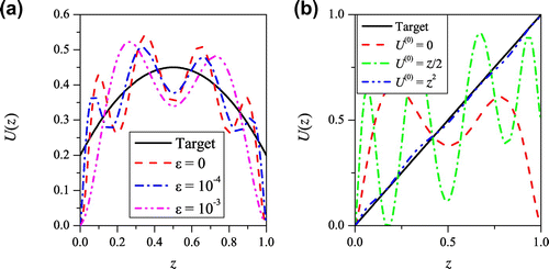
Fig. 4 (a) Reconstruction of target drift $U(z)=0.2+z(1-z)$ with initial guess $U^{(0)}=0$ and starting position $x=0$ for different noise levels $\mathit{\epsilon }$. Algorithm parameters were $N_1=2\times {10}^4$, $T_m=10$, $M=100$, $N=40$. (b) Reconstruction of target drift $U(z)=z$ with different initial guesses. Algorithm parameters were $N_1=2\times {10}^4$, $T_m=10$, $\mathit{\epsilon }={10}^{-6}$, $M=100$, $N=40$.

In Equation (17(17) $$\begin{array}{ccc}\hfill A& =\hfill & \hfill \frac{w_1(z,\mathit{\lambda })W(z)}{w_0(z,\mathit{\lambda })w_{1,z}(z,\mathit{\lambda })-w_1(z,\mathit{\lambda })w_{0,z}(z,\mathit{\lambda })},\\ \hfill B& =\hfill & \hfill \frac{w_0(z,\mathit{\lambda })W(z)}{w_0(z,\mathit{\lambda })w_{1,z}(z,\mathit{\lambda })-w_1(z,\mathit{\lambda })w_{0,z}(z,\mathit{\lambda })},\end{array}$$(17) ), we see that since $H(x,z,\mathit{\lambda })\frac{\text{d}w(z,\mathit{\lambda })}{\text{d}z}=0$ when $z=0$ and $z=1$, rows $1$ and $N+1$ of $J^T$ in (53) consist only of zeros, and columns $1$ and $N+1$ of $J$ consists only of zeros. Therefore, (52) implies that(46) $$\begin{array}{c}\hfill \mathit{\delta }U(z_0)=\mathit{\delta }U(z_N)=0,\end{array}$$(46) and boundary values of the iterates do not change. In Figure 4(a) the exact solution has $U(1)=U(0)=0.2$ and our method fails to converge to the exact solution even for perfectdata. Instead, because the initial guess is $U^{(0)}(z)\equiv 0$, the end points of the solution are pinned at zero and the rest of the solution oscillates about the target $U$. Like all Newton methods, the choice of initial guess is vital to the success of our algorithm and this is illustrated in (b). For initial guesses that have $U(1)\ne 1$, the method is unable to reconstruct even basic features of $U(z)$. However, when $U^{(0)}=z^2$, the method quickly converges to the target drift.

We did attempt to reconstruct drift functions from noisy FPTDs generated by numerically integrating the SDE (1(1) $$\begin{array}{c}\hfill \text{d}Y(t)=U(Y(t))\text{d}t+\sqrt{2D}\text{d}W(t),\end{array}$$(1) ) using a basic Euler–Maruyama method. However, there are(at least) two sources of error associated with sampling $w(x,t)$ in this way. Thefirst is related to the finite $\mathrm{\Delta }t$ discretization of the SDE; this method also over predictsthe first passage times.[28] The second is due to the finite sample size. When we used$\mathrm{\Delta }t={10}^{-5}$ and 4,000 first passage times (which took about 1.5 hours to generate on a quad core Intel Xeon 2 GHz workstation), the error in $\stackrel{\sim }{w}(0,s)$ was about 0.005 which waslarge enough to prevent convergence of the Levenberg–Marquardt method: ourmethod is extremely sensitive to small amounts of noise in the Laplace-transformeddata.

In Figure 2, data with $\mathit{\epsilon }=O({10}^{-5}),N_1=O({10}^4),T_m\approx 5$ usually produced convergent results; these noise parameters for the artificial data correspond to $\stackrel{\sim }{\mathit{\eta }}(\mathit{\lambda })=O({10}^{-5})$ in Equation (54). Unfortunately, we found that it was extremely time consuming to generate a FPTD through the SDE whose Laplace transform is accurate to $O({10}^{-5})$. Since the error in the Laplace-transformed data scales as the inverse square-root of the sample size, while the time taken to generate the data scales linearly with the sample size, we estimate that it would take about ${10}^9$ samples (with $\mathrm{\Delta }t={10}^{-5}$) to obtain FPTD data that is accurate to $O({10}^{-5})$. Therefore, generating ${10}^9$ samples would take about 40 years on our workstation. We leave as future work the implementation of more advanced methods [28, 29] that can simulate diffusive FPTDs more efficiently.

Conclusions

In this paper, we studied the reconstruction of a drift function in a Brownian motion from the Laplace transform of its FPTD. Our main contributions are a proof that the linearized inverse problem is ill-posed and a numerical method based on the Levenberg–Marquardt method. This method allows drift reconstruction to be implemented from artificial data, generated by adding Gaussian noise to a solution of the forward problem.

Our numerical method is able to reconstruct simple drift functions for low noise levels. Furthermore, as with many Newton-type methods, convergence is contingent on a suitable initial guess. In particular, unless the initial guess already takes the correct values at the endpoints, the iterates do not converge.

We see our future work as consisting of three main parts. First, the inverse problem should be solved using exit time data generated by the SDE (1(1) $$\begin{array}{c}\hfill \text{d}Y(t)=U(Y(t))\text{d}t+\sqrt{2D}\text{d}W(t),\end{array}$$(1) ). From our results so far, we anticipate that the Brownian dynamics must be simulated quickly and accurately in order to generate exit time distributions with sufficiently low levels of noise. Alternatively, other efficient methods to sample from the FPTD must be developed.

Second, it remains to establish whether the assumption of $U(Y)=U(1-Y)$ is sufficient to guarantee uniqueness of the inverse problem (10(10) $$\begin{array}{c}\hfill \mathcal{J}\mathit{\delta }{U}^{(k)}=w_{\mathrm{data}}(x_0,\mathit{\lambda })-\mathcal{A}[U^{(k)}]\equiv \mathit{\delta }{w}^{(k)},\end{array}$$(10) )–(12(12) $$\begin{array}{c}\hfill ({\mathcal{J}}^{\ast }\mathcal{J}+{\mathit{\alpha }}_k\mathcal{I})\mathit{\delta }{U}_{{\mathit{\alpha }}_k}^{(k)}={\mathcal{J}}^{\ast }\mathit{\delta }{w}^{(k)},\end{array}$$(12) ). When $U$ is not symmetric, we showed in corollary 1 that $U$ is not unique. In particular, if the starting position$x=0$, $U(Y)$ and $U(1-Y)$ generate exactly the same distribution of first passagetimes.

Finally, our numerical method should be extended so that it can recover drift functions that have non-zero boundary values. An important first step would be to establish the behaviour of $H\frac{\text{d}w}{\text{d}z}$ in (43(43) $$\begin{array}{c}\hfill w_n(x,\mathit{\lambda })=w_p(x,\mathit{\lambda })+\stackrel{\sim }{\mathit{\eta }}(\mathit{\lambda }),\end{array}$$(43) ) as $z\to 0,1$.

Acknowledgments

The author thanks Fioralba Cakoni and Tom Chou for helpful discussions. This work was supported by the University of Delaware Research Foundation (UDRF).

Inequality for uniform continuity

In this appendix, we prove the inequality (47(47) $$\begin{array}{c}\hfill \begin{array}{cc}|F(\mathit{\lambda }+h)-F(\mathit{\lambda })|\le \hfill & |F(\mathit{\lambda }+h)e^{\sqrt{\mathit{\lambda }+h}(1-x)}-F(\mathit{\lambda })e^{\sqrt{\mathit{\lambda }}(1-x)}|e^{-\sqrt{\mathit{\lambda }+h}(1-x)}\hfill \\ \hfill & +|F(\mathit{\lambda })|(1-e^{-[\sqrt{\mathit{\lambda }+h}-\sqrt{\mathit{\lambda }}](1-x)}).\hfill \end{array}\end{array}$$(47) ). Let $F(\mathit{\lambda })\equiv H(x,z,\mathit{\lambda })\frac{\text{d}w(z,\mathit{\lambda })}{\text{d}z}$ where for ease of notation, we omit the $x$ and $z$ dependence in $F$. Then for $h>0$,$$\begin{array}{cc}\hfill & |F(\mathit{\lambda }+h)e^{\sqrt{\mathit{\lambda }+h}(1-x)}-F(\mathit{\lambda })e^{\sqrt{\mathit{\lambda }}(1-x)}|\hfill \\ \hfill & =\hfill & \hfill |F(\mathit{\lambda }+h)e^{\sqrt{\mathit{\lambda }+h}(1-x)}-F(\mathit{\lambda })e^{\sqrt{\mathit{\lambda }+h}(1-x)}+F(\mathit{\lambda })e^{\sqrt{\mathit{\lambda }+h}(1-x)}-F(\mathit{\lambda })e^{\sqrt{\mathit{\lambda }}(1-x)}|,\\ \hfill & \ge \hfill & \hfill e^{\sqrt{\mathit{\lambda }+h}(1-x)}|F(\mathit{\lambda }+h)-F(\mathit{\lambda })|-|F(\mathit{\lambda })|(e^{\sqrt{\mathit{\lambda }+h}(1-x)}-e^{\sqrt{\mathit{\lambda }}(1-x)}).\end{array}$$Therefore,(47) $$\begin{array}{c}\hfill \begin{array}{cc}|F(\mathit{\lambda }+h)-F(\mathit{\lambda })|\le \hfill & |F(\mathit{\lambda }+h)e^{\sqrt{\mathit{\lambda }+h}(1-x)}-F(\mathit{\lambda })e^{\sqrt{\mathit{\lambda }}(1-x)}|e^{-\sqrt{\mathit{\lambda }+h}(1-x)}\hfill \\ \hfill & +|F(\mathit{\lambda })|(1-e^{-[\sqrt{\mathit{\lambda }+h}-\sqrt{\mathit{\lambda }}](1-x)}).\hfill \end{array}\end{array}$$(47)

References

- Fuhrmann A, Anselmetti D, Ros R, Getfert S, Reimann P. Refined procedure of evaluating experimental single-molecule force spectroscopy data. Phys. Rev. E. 2008;77:031912–1-31912-10.
- GetfertS, EvstigneevM, ReimannP. Single-molecule force spectroscopy: practical limitations beyond Bell’s model. Physica A. 2009;388:1120–1132.
- Getfert S, Reimann P. Suppression of thermally activated escape by heating. Phys. Rev. E. 2009;80:030101–1-030101-4.
- HeymannB, GrubmüllerH. Dynamic force spectroscopy of molecular adhesion bonds. Phys. Rev. Lett. 2000;84:6126–6129.
- BalseraM, StepaniantsS, IzrailevS, OonoY, SchultenK. Reconstructing potential energy functions from simulated force-induced unbinding processes. Biophys. J. 1997;73:1281–1287.
- DudkoOK. Single-molecule mechanics: new insights from the escape-over-a-barrier problem. Proc. Nat. Acad. Sci. U.S.A. 2009;106:8795–8796.
- DudkoOK, HummerG, SzaboA. Theory, analysis, and interpretation of single-molecule force spectroscopy experiments. Proc. Nat. Acad. Sci. U.S.A. 2008;105:15755–15760.
- HummerG, SzaboA. Kinetics from nonequilibrium single-molecule pulling experiments. Biophys. J. 2003;85:5–15.
- FreundLB. Characterizing the resistance generated by a molecular bond as it is forcibly separated. Proc. Nat. Acad. Sci. U.S.A. 2009;22:8818–8823.
- GardinerCW. Handbook of stochastic methods. Berlin: Springer; 1985.
- BorgG. Eine Umkehrung der Sturm-Liouvilleschen Eigenwertaufgabe. Acta Math. 1946;78:1–96.
- McLaughlinJR. Analytical methods for recovering coefficients in differential equations from spectral data. SIAM Rev. 1986;28:53–72.
- BrownBM, SamkoVS, KnowlesIW, MarlettaM. Inverse spectral problem for the Sturm-Liouville equation. Inverse Probl. 2003;19:235–252.
- RundellW, SacksPE. The reconstruction of Sturm-Liouville operators. Inverse Probl. 1992;8:457–482.
- Zhou S, Cui M. Determination of unknown coefficients in parabolic equations. J. Heat Transfer. 2009;131:111303–1-111303-6.
- BalG, ChouT. On the reconstruction of diffusions from first-exit time distributions. Inverse Probl. 2003;20:1053–1065.
- LipmanEA, SchulerB, BakajinO, EatonWA. Single-molecule measurement of protein folding kinetics. Science. 2003;301:1233–1235.
- MassonJ-B, CasanovaD, TürkcanS, VoisinneG, PopoffM, VergassolaM, AlexandrouA. Inferring maps of forces inside cell membrane microdomains. Phys. Rev. Lett. 2009;102:1–4.
- Fok P-W, Chou T. Reconstruction of potential energy profiles from multiple rupture time distributions. Proc. R. Soc. London, Ser. A. 2010;466:3479–3499.
- Groetsch CW. Integral equations of the first kind, inverse problems and regularization: a crash course. J. Phys.: Conf. Ser. 2007;73:45–54.
- KressR. Linear integral equations. Berlin: Springer-Verlag; 1989.
- EnglHW, HankeM, NeubauerA. Regularization of inverse problems. Dordrecht: Kluwer; 1996.
- HankeM. A regularizing Levenberg-Marquardt scheme with applications to inverse groundwater filtration problems. Inverse Probl. 1997;13:79.
- ChipotM. Elliptic equations: an introductory course. Basel: Birkhäuser Verlag; 2009.
- TrefethenLN. Spectral methods in Matlab. Philadelphia (PA): SIAM; 2000.
- HohageT. Logarithmic convergence rates of the iteratively regularized Gauss-Newton method for an inverse potential and an inverse scattering problem. Inverse Probl. 1997;13:1279.
- Colton D, Engl HW, Louis AK, McLaughlin JR, Rundell W, editors. Surveys on solution methods for inverse problems. New York: Springer; 2000.
- BuchmannFM. Simulation of stopped diffusions. J. Comput. Phys. 2005;202:446–462.
- GiraudoMT, SacerdoteL. An improved technique for the simulation of first passage times for diffusion processes. Comm. Statist. Simulation Comput. 1999;28:1135–1163.