Rapid identification of material properties of the interface tissue in dental implant systems using reduced basis method

Abstract

This paper proposes a rapid inverse analysis approach based on the reduced basis (RB) method and the Levenberg–Marquardt–Fletcher algorithm to identify the ‘unknown’ material properties: Young’s modulus and stiffness-proportional Rayleigh damping coefficient of the interfacial tissue between a dental implant and the surrounding bones. In the forward problem, a finite element approximation for a three-dimensional dental implant-bone model is first built. A RB approximation is then established by using a proper orthogonal decomposition – Greedy algorithm and the Galerkin projection to enable extremely fast and reliable computation of displacement responses for a range of material properties. In the inverse analysis, the RB approximation for the dental implant-bone model are incorporated in the Levenberg–Marquardt–Fletcher algorithm to enable rapid identification of the unknown material properties. Numerical results are presented to demonstrate the efficiency and robustness of the proposed method.

Keywords:

• second-order hyperbolic partial differential equations
• reduced basis method
• inverse analysis
• Levenberg–Marquardt–Fletcher algorithm
• material characterization
• POD–Greedy algorithm

Introduction

Osseointegration is a slow process of structural and functional connection between living bone and dental implant surfaces.[1] In the osseointegration process, the conditions of implant-bone interfacial tissues are very important as they reflect the bone remodelling and the stability of dental implant-bone structures. Understanding these conditions allows clinicians to decide on effective treatments. From a mechanical viewpoint, the material properties of the interfacial tissues are the most important condition indicator as they determine the biomechanical behaviour and stability of implant-bone structures.

A number of methods have been proposed to identify the tissue properties of dental implant-bone structures with in vitro and in vivo studies.[2] Examples are the clinical percussion testing (impact testing),[3, 4] the radio-graphic observation method and the resonance frequency analysis (RFA).[5, 6] Among these methods, the RFA is adopted by most researchers and is extensively used in many dental implant researches to date.[6–9] In the area of non-destructive evaluation, there are other methods which were shown successful with some levels in identifying the tissues properties of dental implant-bone structures. An example of such methods is the inverse analysis method.[10–12] However, either the method was based on the finite element method (FEM) (which is time consuming) [10, 11] or has focused on the frequency-domain (which is not really real-time analysis).[12] Therefore, they are not convenient for clinicians.

The FEM has been widely employed to solve elasticity equations in dental implant studies (e.g. [9, 13, 14]). Although the FEM is a very useful and powerful tool in the inverse analysis context, it can be time consuming because the complexity of implant-bone structures requires a very large number of elements and because many forward problems need to be solved. The total CPU time using FEM can be so long that real-time identification is not possible. A fast forward solver is therefore essential to enable real-time inverse analysis, thereby providing clinicians with the immediate knowledge of the conditions of the implant-bone interfacial tissues.

The reduced basis (RB) method is a model order reduction framework for rapid and reliable evaluation of functional outputs of solutions of parametrized partial differential equations (PDEs). These PDEs depend on an input parameter vector that includes geometry parameters and/or material properties. The RB method was developed for elliptic PDEs,[15, 16] parabolic PDEs,[17] hyperbolic PDEs,[18] the viscous Burgers’ equation [19] and the steady incompressible Navier-Stokes equation.[20] Recently, Liu et al. developed a RB method for elasticity problems based on a smooth Galerkin projection [21] which can provide an upper bound to the exact solution, while the original RB method provides a lower bound to the exact solution. The computational efficiency of the RB method was demonstrated significantly higher than that of the FEM in the inverse analysis context.[22]

Several methods have been proposed for solving inverse problems in non-destructive evaluation. They include global search algorithms such as the genetic algorithm, simulated annealing, neural network and local gradient-based algorithms such as the gradient descent, Gauss–Newton or Levenberg–Marquardt method. Applications of the neural network for dental implant inverse problems can be found in [10, 11]. Recently, Zaw et al. [12] developed a technique to determine non-invasively the material properties of implant-bone interfacial tissues by using the RB method in combination with the neural network in the frequency domain. However, time-domain applications have not yet been considered. In addition, the Levenberg–Marquardt algorithm has not been applied to the dental implant inverse problems, although this algorithm was widely used to solve other important inverse problems.[23–26]

In this paper, we introduce an inverse analysis approach for rapid identification of the material properties of the interfacial tissues. There are two main components in our approach: the RB method and the Levenberg–Marquardt–Fletcher algorithm. We first develop a RB approximation for linear elastodynamics that govern the structural responses of a dental implant-bone model. This is achieved by using a proper orthogonal decomposition (POD)–Greedy algorithm, the Galerkin projection and an offline–online computational procedure. The RB approximation provides extremely fast and reliable calculation of displacement responses for a range of material properties. We then incorporate the RB approximation into the Levenberg–Marquardt–Fletcher algorithm to enable rapid identification of the unknown material properties. Finally, the efficiency and robustness of the proposed method are demonstrated for a real in vitro model.

The paper is organized as follows. In Section 2, we introduce a real in vitro model and associated finite element approximations. In Section 3, we develop the RB approximation and present some numerical results. In Section 4, we describe the proposed inverse analysis approach and present numerical results to demonstrate its efficiency and robustness. Finally, we provide some concluding remarks in Section 5.

Problem description and finite element approximation

Models and approximations

The real in vitro model

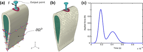
We consider a real in vitro model shown in Figure 1(a). The bone is made of the bovine rib of a mature specimen obtained commercially. The bone is composed of two subparts: the cortical bone and the cancellous bone. The thickness of the cortical bone is 2mm. A cylindrical implant socket whose diameter of 6.5mm and depth of 15mm is drilled into the bone. A cylindrical dental implant whose diameter of 4mm and length of 12mm is inserted into the drilled hole. A layer of 2.5mm thickness surrounding the dental implant is the interfacial tissue whose material properties need to be identified in the osseointegration process. Finally, a stainless steel screw is screwed tightly into the dental implant. The screw is modelled as a cylinder that has 1.5mm in diameter and 12.5mm in length, respectively.

Fig. 1 The real in vitro model (a) and the 3d simplified FEM model with sectional view (b).

Fig. 2 Output point, applied load and boundary conditions (a), meshed model in ABAQUS (b) and time history of load (c).

The simplified 3d FEM model

Figure 1(b) presents a simplified 3D dental implant-bone model that simulates the real in vitro model shown in Figure 1(a). The geometry of the simplified dental implant-bone model is constructed by using SolidWorks 2005. The physical domain $\mathrm{\Omega }$ consists of five regions: the outermost cortical bone ${\mathrm{\Omega }}_1$, the cancellous bone ${\mathrm{\Omega }}_2$, the interfacial tissue ${\mathrm{\Omega }}_3$, the dental implant ${\mathrm{\Omega }}_4$ and the stainless steel screw ${\mathrm{\Omega }}_5$. The 3D simplified model is then meshed and analysed in the software ABAQUS/CAE version 6.9-1. A dynamic force opposite to the $x$-direction is then applied to the body of the screw as shown in Figure 2(a). The time history of the applied load is also presented in Figure 2(c). The output of interest is defined as the displacement responses of a point on the head of the screw. The Dirichlet boundary condition $(\mathit{\partial }{\mathrm{\Omega }}^D)$ is specified in the bottom-half of the simplified model as illustrated in Figure 2(a). As shown in Figure 2(b) the finite element mesh consists of 9655 nodes and 52585 four-node tetrahedral solid elements. The coinciding nodes of the contact surfaces between different regions (the regions ${\mathrm{\Omega }}_1$, ${\mathrm{\Omega }}_2$, ${\mathrm{\Omega }}_3$, ${\mathrm{\Omega }}_4$, ${\mathrm{\Omega }}_5$) are assumed to be rigidly fixed, i.e. the displacements in the $x$-, $y$- and $z$-directions are all set to be the same for the same coinciding nodes.

Table 1 Material properties of the dental implant-bone structure.

Domain	Layers	E (Pa)	$\mathit{\nu }$	$\mathit{\rho }(\mathrm{g}{\mathit{mm}}^{-3})$	$\mathit{\beta }$
${\mathrm{\Omega }}_1$	Cortical bone	$2.3162\times {10}^{10}$	0.371	$1.8601\times {10}^{-3}$	$3.38\times {10}^{-6}$
${\mathrm{\Omega }}_2$	Cancellous bone	$8.2345\times {10}^8$	0.3136	$7.1195\times {10}^{-4}$	$6.76\times {10}^{-6}$
${\mathrm{\Omega }}_3$	Tissue	E	0.3155	$1.055\times {10}^{-3}$	$\mathit{\beta }$
${\mathrm{\Omega }}_4$	Titan implant	$1.05\times {10}^{11}$	0.32	$4.52\times {10}^{-3}$	$5.1791\times {10}^{-10}$
${\mathrm{\Omega }}_5$	Stainless steel screw	$1.93\times {10}^{11}$	0.305	$8.027\times {10}^{-3}$	$2.5685\times {10}^{-8}$

We assume that the regions ${\mathrm{\Omega }}_i,1\le i\le 5$, of the simplified model are homogeneous and isotropic1. The material properties: the Young’s moduli, Poisson’s ratios and densities of these regions are presented in Table 1 [12, 27]. In order to simulate the damping of the system, the Rayleigh damping assumption [28] is used in our analysis. Each region shall have their own pair values of ${\mathit{\alpha }}_i$ – the mass-proportional damping coefficients which represent the contribution of the mass matrices into the damping matrices of interest and ${\mathit{\beta }}_i$ ($i=1,\dots ,5$) – the stiffness-proportional damping coefficients which represent the contribution of the stiffness matrices into the damping matrices, respectively. We conducted a sensitivity analysis for the values of ${\mathit{\alpha }}_i,1\le i\le 5$, to the displacement output and found that they do not affect the displacement output of our problem. This means that our current problem setting is stiffness dominated and the damping being used here, in essence, is Kelvin–Voigt damping. Based on this finding, ${\mathit{\beta }}_i,1\le i\le 5$, have the values as presented in the last column of Table 1 such that$${\mathbf{C}}_i={\mathit{\beta }}_i{\mathbf{A}}_i,i=1,\dots ,5,$$where ${\mathbf{C}}_i$ and ${\mathbf{A}}_i$ are the FEM damping and stiffness matrices of each region, respectively. We also note in Table 1 that the Young’s modulus $E$ and the stiffness-proportional Rayleigh damping coefficient $\mathit{\beta }$ of the region ${\mathrm{\Omega }}_3$ ($E_3$,${\mathit{\beta }}_3$) are ‘unknown’ material parameters that need to be identified.

The 3D simplified dental implant-bone problem is solved by taking two important considerations. Firstly, the loading applied to the head of the screw is extremely small. Hence, the deformation of the whole structure is small and shall be governed by linear elastodynamics.[11–13] Secondly, all layers except the tissue (i.e. the cortical bone, the cancellous bone, the implant and the screw) are very hard and the tissue is the only soft layer considered. Therefore, the output displacement responses of the system are mostly affected by the material properties of the tissue layer only.

Here, we aim to identify the ‘unknown’ material properties of the interfacial tissue, namely the Young’s modulus $E$ and the stiffness-proportional Rayleigh’s damping coefficient $\mathit{\beta }$, from the displacement responses of the dental-implant bone structure due to the excitation force. Our analysis procedure consists of two parts: forward analysis and inverse analysis. In the forward analysis, the output displacement responses are determined for a range of input system parameters $(E,\mathit{\beta })$ for which we need to build a RB model. The inverse analysis determines $(E_{\mathrm{true}},{\mathit{\beta }}_{\mathrm{true}})$ from a given measurement of output displacement response of the dental implant structure when it is excited by the applied load.

Finite element approximation

Formulations and definitions

We consider a spatial domain $\mathrm{\Omega }\in {\mathbb{R}}^3$ with a boundary $\mathit{\partial }\mathrm{\Omega }$. We denote the Dirichlet portion of the boundary by ${\mathrm{\Gamma }}_i^D,1\le i\le 3$. We then introduce the Hilbert spaces(1a) $$\begin{array}{c}\hfill Y^e=\{v\equiv (v_1,v_2,v_3)\in {(H^1(\mathrm{\Omega }))}^3|v_i=0\mathrm{on}{\mathrm{\Gamma }}_i^D,i=1,2,3\},\end{array}$$(1a) (1b) $$\begin{array}{c}\hfill X^e={(L^2(\mathrm{\Omega }))}^3.\end{array}$$(1b) Here, $H^1(\mathrm{\Omega })=\{v\in L^2(\mathrm{\Omega })|\nabla v\in {(L^2(\mathrm{\Omega }))}^3\}$ where $L^2(\mathrm{\Omega })$ is the space of square-integrable functions over $\mathrm{\Omega }$. We equip our spaces with inner products and associated norms ${(·,·)}_{Y^e}$$({(·,·)}_{X^e})$ and $\parallel ·{\parallel }_{Y^e}=\sqrt{{(·,·)}_{Y^e}}$$(\parallel ·{\parallel }_{X^e}=\sqrt{{(·,·)}_{X^e}})$, respectively; a typical choice is(2a) $$\begin{array}{c}\hfill {(w,v)}_{Y^e}={\int }_{\mathrm{\Omega }}\frac{\mathit{\partial }{w}_i}{\mathit{\partial }{x}_j}\frac{\mathit{\partial }{v}_i}{\mathit{\partial }{x}_j}+w_i{v}_i,\end{array}$$(2a) (2b) $$\begin{array}{c}\hfill {(w,v)}_{X^e}={\int }_{\mathrm{\Omega }}{w}_i{v}_i,\end{array}$$(2b) where the summation over repeated indices is assumed.

We next define our parameter set $\mathcal{D}\in {\mathbb{R}}^P$, a typical point in which shall be denoted $\mathit{\mu }\equiv ({\mathit{\mu }}_1,\dots ,{\mathit{\mu }}_P)$. We then define the parametrized bilinear forms $a$ in $Y^e$, $a:Y^e\times Y^e\times \mathcal{D}\to \mathbb{R}$; $m,c,f,\ell$are continuous bilinear and linear forms in $X^e$, $m:X^e\times X^e\to \mathbb{R}$, $c:X^e\times X^e\times \mathcal{D}\to \mathbb{R}$, $f:X^e\to \mathbb{R}$ and $\ell :X^e\to \mathbb{R}$.

The ‘exact’ linear elasticity problem is stated follows: given a parameter $\mathit{\mu }\in \mathcal{D}\subset {\mathbb{R}}^P$, we evaluate the output of interest(3) $$\begin{array}{c}\hfill s^e(\mathit{\mu },t)=\ell (u^e(\mathit{\mu },t)),t\in [0,T],\end{array}$$(3) where the field variable $u^e(\mathit{\mu },t)\in Y^e$ satisfies the weak form of the $\mathit{\mu }$-parametrized hyperbolic PDE$$m(\frac{{\mathit{\partial }}^2{u}^e(\mathit{\mu },t)}{\mathit{\partial }{t}^2},v)+c(\frac{\mathit{\partial }{u}^e(\mathit{\mu },t)}{\mathit{\partial }t},v;\mathit{\mu })+a(u^e(\mathit{\mu },t),v;\mathit{\mu })=g(t)f(v),\forall v\in Y^e,t\in [0,T],$$with initial conditions $u^e(\mathit{\mu },t^0)=0$, $\frac{\mathit{\partial }{u}^e(\mathit{\mu },t^0)}{\mathit{\partial }t}=0$.

We next introduce a reference finite element approximation space $Y\subset Y^e(\subset X^e)$ of dimension $\mathcal{N}$; we further define $X\equiv X^e$. Note that $Y$ and $X$ shall inherit the inner product and norm from $Y^e$ and $X^e$, respectively. Our ‘true’ finite element approximation $u(\mathit{\mu },t)\in Y$ to the ‘exact’ problem2 is stated as:$$m(\frac{{\mathit{\partial }}^{2}u(\mathit{\mu },t)}{\mathit{\partial }{t}^2},v)+c(\frac{\mathit{\partial }u(\mathit{\mu },t)}{\mathit{\partial }t},v;\mathit{\mu })+a(u(\mathit{\mu },t),v;\mathit{\mu })=g(t)f(v),\forall v\in Y,t\in [0,T],$$with initial conditions $u(\mathit{\mu },t^0)=0$, $\frac{\mathit{\partial }u(\mathit{\mu },t^0)}{\mathit{\partial }t}=0$; we then evaluate the output of interest(4) $$\begin{array}{c}\hfill s(\mathit{\mu },t)=\ell (u(\mathit{\mu },t)),t\in [0,T].\end{array}$$(4) The RB approximation shall be built upon our reference finite element approximation, and the RB error will thus be evaluated with respect to $u(\mathit{\mu },t)\in Y$. Clearly, our methods must remain computationally efficient and stable as $\mathcal{N}\to \infty$.

We shall assume that the bilinear forms $a(·,·;\mathit{\mu })$ and $m(·,·;\mathit{\mu })$ are continuous,(5a) $$\begin{array}{c}\hfill a(w,v;\mathit{\mu })\le \mathit{\gamma }\parallel w{\parallel }_Y\parallel v{\parallel }_Y\le {\mathit{\gamma }}_0\parallel w{\parallel }_Y\parallel v{\parallel }_Y,\forall w,v\in Y,\forall \mathit{\mu }\in \mathcal{D},\end{array}$$(5a) (5b) $$\begin{array}{c}\hfill m(w,v;\mathit{\mu })\le \mathit{\rho }\parallel w{\parallel }_X\parallel v{\parallel }_X\le {\mathit{\rho }}_0\parallel w{\parallel }_X\parallel v{\parallel }_X,\forall w,v\in Y,\forall \mathit{\mu }\in \mathcal{D},\end{array}$$(5b) coercive,(6a) $$\begin{array}{c}\hfill 0\le {\mathit{\alpha }}_0\le \mathit{\alpha }(\mathit{\mu })\equiv \underset{v\in Y}{\inf }\frac{a(v,v;\mathit{\mu })}{\parallel v{\parallel }_Y^2},\forall \mathit{\mu }\in \mathcal{D},\end{array}$$(6a) (6b) $$\begin{array}{c}\hfill 0\le {\mathit{\sigma }}_0\le \mathit{\sigma }(\mathit{\mu })\equiv \underset{v\in Y}{\inf }\frac{m(v,v;\mathit{\mu })}{\parallel v{\parallel }_X^2},\forall \mathit{\mu }\in \mathcal{D};\end{array}$$(6b) and symmetric $a(v,w;\mathit{\mu })=a(w,v;\mathit{\mu }),\forall w,v\in Y,\forall \mathit{\mu }\in \mathcal{D}$ and $m(v,w;\mathit{\mu })=m(w,v;\mathit{\mu }),$$\forall w,v\in X,\forall \mathit{\mu }\in \mathcal{D}$. (We (plausibly) suppose that ${\mathit{\gamma }}_0,{\mathit{\rho }}_0,{\mathit{\alpha }}_0$ and ${\mathit{\sigma }}_0$ may be chosen independent of $\mathcal{N}$ [17]). We also require that the linear forms $f(v):Y\to \mathbb{R}$ and $\ell (v):Y\to \mathbb{R}$ be bounded with respect to $\parallel ·{\parallel }_Y$ and $\parallel ·{\parallel }_X$, respectively.

With respect to our particular dental implant problem described in Section Section32.1.2 the actual integral forms of the linear and bilinear forms are defined as:(7a) $$\begin{array}{c}\hfill m(w,v)=\sum _{r=1}^5{\int }_{{\mathrm{\Omega }}_r}{\mathit{\rho }}_r{w}_i{v}_i,\end{array}$$(7a) (7b) $$\begin{array}{c}\hfill a(w,v;\mathit{\mu })=\sum _{r=1,r\ne 3}^5{\int }_{{\mathrm{\Omega }}_r}\frac{\mathit{\partial }{v}_i}{\mathit{\partial }{x}_j}{C}_{\mathit{ijkl}}^r\frac{\mathit{\partial }{w}_k}{\mathit{\partial }{x}_l}+{\mathit{\mu }}_1{\int }_{{\mathrm{\Omega }}_3}\frac{\mathit{\partial }{v}_i}{\mathit{\partial }{x}_j}{C}_{\mathit{ijkl}}^3\frac{\mathit{\partial }{w}_k}{\mathit{\partial }{x}_l},\end{array}$$(7b) (7c) $$\begin{array}{c}\hfill c(w,v;\mathit{\mu })=\sum _{r=1,r\ne 3}^5{\mathit{\beta }}_r{\int }_{{\mathrm{\Omega }}_r}\frac{\mathit{\partial }{v}_i}{\mathit{\partial }{x}_j}{C}_{\mathit{ijkl}}^r\frac{\mathit{\partial }{w}_k}{\mathit{\partial }{x}_l}+{\mathit{\mu }}_2{\mathit{\mu }}_1{\int }_{{\mathrm{\Omega }}_3}\frac{\mathit{\partial }{v}_i}{\mathit{\partial }{x}_j}{C}_{\mathit{ijkl}}^3\frac{\mathit{\partial }{w}_k}{\mathit{\partial }{x}_l},\end{array}$$(7c) (7d) $$\begin{array}{c}\hfill f(v)={\int }_{{\mathrm{\Gamma }}_n^N}v,\end{array}$$(7d) for all $w,v\in Y$, $\mathit{\mu }\in \mathcal{D}$. Here, the ‘unknown’ parameter $\mathit{\mu }=({\mathit{\mu }}_1,{\mathit{\mu }}_2)\equiv (E,\mathit{\beta })$ belongs to the region ${\mathrm{\Omega }}_3$. $C_{\mathit{ijkl}}^r$ is the constitutive elasticity tensor for isotropic materials and it is expressed in terms of the Young’s modulus $E$ and Poisson’s ratio $\mathit{\nu }$ of each region ${\mathrm{\Omega }}_r,1\le r\le 5$, respectively. ${\mathrm{\Gamma }}_n^N$ is the point where the load is applied as shown in Figure 2(a). The material properties $E_r$ and ${\mathit{\beta }}_r,1\le r\le 5,r\ne 3$; ${\mathit{\nu }}_r$ and ${\mathit{\rho }}_r$, $1\le r\le 5$ are defined as in Table 1.

From (9b) and (9c), we find that $a$ and $c$ depend affinely on the parameter $\mathit{\mu }$ and that they can be expressed as:(8a) $$\begin{array}{c}\hfill a(w,v;\mathit{\mu })=\sum _{q=1}^{Q_a}{\mathrm{\Theta }}_a^q(\mathit{\mu })a^q(w,v),\forall w,v\in Y,\mathit{\mu }\in \mathcal{D},\end{array}$$(8a) (8b) $$\begin{array}{c}\hfill c(w,v;\mathit{\mu })=\sum _{q=1}^{Q_c}{\mathrm{\Theta }}_c^q(\mathit{\mu })c^q(w,v),\forall w,v\in Y,\mathit{\mu }\in \mathcal{D}.\end{array}$$(8b) Here, the smooth functions ${\mathrm{\Theta }}_a^1(\mathit{\mu })=1$, ${\mathrm{\Theta }}_a^2(\mathit{\mu })={\mathit{\mu }}_1$; ${\mathrm{\Theta }}_c^1(\mathit{\mu })=1$, ${\mathrm{\Theta }}_c^2(\mathit{\mu })={\mathit{\mu }}_1{\mathit{\mu }}_2$ depend on $\mathit{\mu }$. But the bilinear forms $a^1(w,v)=\sum _{r=1,r\ne 3}^5{\int }_{{\mathrm{\Omega }}_r}\frac{\mathit{\partial }{v}_i}{\mathit{\partial }{x}_j}{C}_{\mathit{ijkl}}^r\frac{\mathit{\partial }{w}_k}{\mathit{\partial }{x}_l}$, $a^2(w,v)={\int }_{{\mathrm{\Omega }}_3}\frac{\mathit{\partial }{v}_i}{\mathit{\partial }{x}_j}{C}_{\mathit{ijkl}}^3\frac{\mathit{\partial }{w}_k}{\mathit{\partial }{x}_l}$; $c^1(w,v)=\sum _{r=1,r\ne 3}^5{\mathit{\beta }}_r{\int }_{{\mathrm{\Omega }}_r}\frac{\mathit{\partial }{v}_i}{\mathit{\partial }{x}_j}{C}_{\mathit{ijkl}}^r\frac{\mathit{\partial }{w}_k}{\mathit{\partial }{x}_l}$ and $c^2(w,v)={\int }_{{\mathrm{\Omega }}_3}\frac{\mathit{\partial }{v}_i}{\mathit{\partial }{x}_j}{C}_{\mathit{ijkl}}^3$$\frac{\mathit{\partial }{w}_k}{\mathit{\partial }{x}_l}$ do not depend on $\mathit{\mu }$. Finally, we also require that all linear and bilinear forms be independent of time – the system is thus linear time-invariant.[17]

Time discretization

We shall use the Newmark’s scheme with coefficients $(\mathit{\phi }=\frac{1}{2},\mathit{\psi }=\frac{1}{4})$ [29] to approximate the time derivative terms of the ‘true’ statement (5). For time integration: we divide $[0,T]$ into $K$ subintervals of equal lengths $\mathrm{\Delta }t=\frac{T}{K}$, and define $t^k=k\mathrm{\Delta }t,0\le k\le K$. Our finite element approximation is then given by:(9) $$\begin{array}{cc}\hfill & m(u(\mathit{\mu },t^{k+1}),v)+\frac{1}{2}\mathrm{\Delta }tc(u(\mathit{\mu },t^{k+1}),v;\mathit{\mu })+\frac{1}{4}\mathrm{\Delta }{t}^{2}a(u(\mathit{\mu },t^{k+1}),v;\mathit{\mu })\hfill \\ \hfill & =-m(u(\mathit{\mu },t^{k-1}),v)+\frac{1}{2}\mathrm{\Delta }tc(u(\mathit{\mu },t^{k-1}),v;\mathit{\mu })-\frac{1}{4}\mathrm{\Delta }{t}^{2}a(u(\mathit{\mu },t^{k-1}),v;\mathit{\mu })\hfill \\ \hfill & +2m(u(\mathit{\mu },t^k),v)-\frac{1}{2}\mathrm{\Delta }{t}^{2}a(u(\mathit{\mu },t^k),v;\mathit{\mu })\hfill \\ \hfill & +\mathrm{\Delta }{t}^2{g}^{\mathit{eq}}(t^k)f(v),\hfill \\ \hfill & \forall v\in Y,1\le k\le K-1,\hfill \end{array}$$(9) with(10) $$\begin{array}{c}\hfill g^{\mathit{eq}}(t^k)=\frac{1}{4}g(t^{k-1})+\frac{1}{2}g(t^k)+\frac{1}{4}g(t^{k+1}),1\le k\le K-1.\end{array}$$(10) In order to start the procedure (11(11) $$\begin{array}{c}\hfill m(\ddot{u}(\mathit{\mu },t^1),v)+\frac{1}{2}\mathrm{\Delta }tc(\ddot{u}(\mathit{\mu },t^1),v;\mathit{\mu })+\frac{1}{4}\mathrm{\Delta }{t}^{2}a(\ddot{u}(\mathit{\mu },t^1),v;\mathit{\mu })=g(t^1)f(v),\forall v\in Y.\end{array}$$(11) ), $u(\mathit{\mu },t^1)$ is computed as on page 491 of [28]. With the assumptions of $u(\mathit{\mu },t^0)=0$, $\stackrel{·}{u}(\mathit{\mu },t^0)=0$ and $g(t^0)=0$; then $u(\mathit{\mu },t^1)$ is computed from: $u(\mathit{\mu },t^1)=\frac{1}{4}\mathrm{\Delta }{t}^2\ddot{u}(\mathit{\mu },t^1)$, where the acceleration $\ddot{u}(\mathit{\mu },t^1)$ is found from:(11) $$\begin{array}{c}\hfill m(\ddot{u}(\mathit{\mu },t^1),v)+\frac{1}{2}\mathrm{\Delta }tc(\ddot{u}(\mathit{\mu },t^1),v;\mathit{\mu })+\frac{1}{4}\mathrm{\Delta }{t}^{2}a(\ddot{u}(\mathit{\mu },t^1),v;\mathit{\mu })=g(t^1)f(v),\forall v\in Y.\end{array}$$(11) We then evaluate the output from:(12) $$\begin{array}{c}\hfill s(\mathit{\mu },t^k)=\ell (u(\mathit{\mu },t^k)),1\le k\le K.\end{array}$$(12)

RB approximation

The RB method is a cooperative method that is constructed from the FEM. The idea of the RB method is that instead of solving a very time-consuming and expensive FEM system for each input parameter, we would rather proceed with two stages: an offline stage and an online stage. In the offline stage – performed only once, we pre-compute several FEM solutions corresponding to several sets of input parameters (the $S^{\ast }$ set in the following sections) and use these FEM solutions as basis vectors of the RB spaces (the $Y_N$ space in the following sections). Then, in the online stage – performed numerous times, we can compute very rapidly and accurately the solution/ouput of the RB system for a required input parameter by taking a proper linear combination (Galerkin projection) of the RB basis vectors. The computational time and computational cost of the online stage are very cheap because necessary operation counts depend only on the dimension $N$ of the RB spaces rather than the dimension $\mathcal{N}$ of the FEM space and $N\ll \mathcal{N}$. Obviously, we will evaluate the error between the RB solution and the FEM solution as well as the error between the RB output and the FEM output to assess the quality of the RB solution/output with respect to the FEM ones. This kind of error, which is called the ‘RB error’ because it is the error induced by the RB approximation, will be discussed in more detail in Section Section23.3. One can refer to [30] for more information regarding the RB method and all related aspects.

RB method

We introduce the nested samples $S^{\ast }=\{{\mathit{\mu }}_1\in \mathcal{D},{\mathit{\mu }}_2\in \mathcal{D},\dots ,{\mathit{\mu }}_N\in \mathcal{D}\}$, $1\le N\le N_{\max }$, and associated nested Lagrangian RB spaces $Y_N=\mathrm{s}\mathit{pan}\{{\mathit{\zeta }}_n,1\le n\le N\},1\le N\le N_{\max }$, where ${\mathit{\zeta }}_n\in Y_N$, $1\le n\le N_{\max }$ are mutually ${(·,·)}_Y$ – orthonormal RB basis functions. The sets $S^{\ast }$ and $Y_N$ shall be constructed appropriately by the POD–Greedy algorithm described in Section Section33.2.2 afterward. Our RB approximation $u_N(\mathit{\mu },t)$ to $u(\mathit{\mu },t)$ is then obtained by a standard Galerkin projection: given $\mathit{\mu }\in \mathcal{D}$, we now look for $u_N(\mathit{\mu },t)\in Y_N$ satisfies$$m(\frac{{\mathit{\partial }}^2{u}_N(\mathit{\mu },t)}{\mathit{\partial }{t}^2},v)+c(\frac{\mathit{\partial }{u}_N(\mathit{\mu },t)}{\mathit{\partial }t},v;\mathit{\mu })+a(u_N(\mathit{\mu },t),v;\mathit{\mu })=g(t)f(v),\forall v\in Y_N,t\in [0,T].$$We evaluate the associated RB output, $s_N(\mathit{\mu },t)$, from(13) $$\begin{array}{c}\hfill s_N(\mathit{\mu },t)=\ell (u_N(\mathit{\mu },t)),t\in [0,T].\end{array}$$(13) The discrete RB approximation equation of (15(15) $$\begin{array}{c}\hfill s_N(\mathit{\mu },t^k)=\ell (u_N(\mathit{\mu },t^k)),1\le k\le K.\end{array}$$(15) ) is then given by:$$m(u_N(\mathit{\mu },t^{k+1}),v)+\frac{1}{2}\mathrm{\Delta }tc(u_N(\mathit{\mu },t^{k+1}),v;\mathit{\mu })+\frac{1}{4}\mathrm{\Delta }{t}^{2}a(u_N(\mathit{\mu },t^{k+1}),v;\mathit{\mu })=-m(u_N(\mathit{\mu },t^{k-1}),v)+\frac{1}{2}\mathrm{\Delta }tc(u_N(\mathit{\mu },t^{k-1}),v;\mathit{\mu })-\frac{1}{4}\mathrm{\Delta }{t}^{2}a(u_N(\mathit{\mu },t^{k-1}),v;\mathit{\mu })+2m(u_N(\mathit{\mu },t^k),v)-\frac{1}{2}\mathrm{\Delta }{t}^{2}a(u_N(\mathit{\mu },t^k),v;\mathit{\mu })+\mathrm{\Delta }{t}^2{g}^{\mathit{eq}}(t^k)f(v),\forall v\in Y_N,1\le k\le K-1.$$Similar to (13(13) $$\begin{array}{c}\hfill s_N(\mathit{\mu },t)=\ell (u_N(\mathit{\mu },t)),t\in [0,T].\end{array}$$(13) ), with zero initial conditions: $u_N(\mathit{\mu },t^0)=0$, ${\stackrel{·}{u}}_N(\mathit{\mu },t^0)=0$, $g(t^0)$$=0$; $u_N(\mathit{\mu },t^1)$ is calculated from: $u_N(\mathit{\mu },t^1)=\frac{1}{4}\mathrm{\Delta }{t}^2{\ddot{u}}_N(\mathit{\mu },t^1)$, and the RB acceleration ${\ddot{u}}_N(\mathit{\mu },t^1)$ is found from:(14) $$\begin{array}{cc}\hfill m({\ddot{u}}_N(\mathit{\mu },t^1),v)+& \frac{1}{2}\mathrm{\Delta }tc({\ddot{u}}_N(\mathit{\mu },t^1),v;\mathit{\mu })+\frac{1}{4}\mathrm{\Delta }{t}^{2}a({\ddot{u}}_N(\mathit{\mu },t^1),v;\mathit{\mu })=g(t^1)f(v),\hfill \\ \hfill & \forall v\in Y_N.\hfill \end{array}$$(14) Finally, the RB output is evaluated from:(15) $$\begin{array}{c}\hfill s_N(\mathit{\mu },t^k)=\ell (u_N(\mathit{\mu },t^k)),1\le k\le K.\end{array}$$(15)

POD–Greedy sampling procedure

In this section, we present briefly the POD method and then introduce our POD–Greedy sampling algorithm used in this work.

The proper orthogonal decomposition

We aim to generate an optimal (in the mean square error sense) basis set $\{{\mathit{\zeta }}_m{\}}_{m=1}^M$ from any given set of $M_{\max }(\ge M)$ snapshots $\{{\mathit{\xi }}_k{\}}_{k=1}^{M_{\max }}$. To do this, let $V_M=\mathrm{s}\mathit{pan}\{v_1,\dots ,v_M\}\subset \mathrm{s}\mathit{pan}\{{\mathit{\xi }}_1,\dots ,{\mathit{\xi }}_{M_{\max }}\}$ be an ‘arbitrary’ space of dimension $M$. We assume that the space $V_M$ is orthonormal such that $(v_n,v_m)={\mathit{\delta }}_{\mathit{nm}},1\le n,m\le M$ ($(·,·)$ denotes an appropriate inner product and ${\mathit{\delta }}_{\mathit{nm}}$ is the Kronecker delta symbol). The POD space, $W_M=\mathrm{s}\mathit{pan}\{{\mathit{\zeta }}_1,\dots ,{\mathit{\zeta }}_M\}$ is defined as:(16) $$\begin{array}{c}\hfill W_M=\arg \underset{V_M\subset \mathrm{s}\mathit{pan}\{{\mathit{\xi }}_1,\dots ,{\mathit{\xi }}_{M_{\max }}\}}{\min }(\frac{1}{M_{\max }}\sum _{k=1}^{M_{\max }}\underset{{\underset{¯}{\mathit{\alpha }}}^k\in {\mathbb{R}}^M}{\inf }\parallel {\mathit{\xi }}_k-\sum _{m=1}^M{\mathit{\alpha }}_m^k{v}_m{\parallel }^2).\end{array}$$(16) The POD space $W_M$ which is extracted from the given set of snapshots $\{{\mathit{\xi }}_k{\}}_{k=1}^{M_{\max }}$ is the space that best approximate this given set of snapshots and can be written as $W_M=\mathrm{POD}(\{{\mathit{\xi }}_1,\dots ,{\mathit{\xi }}_{M_{\max }}\},M)$. We can construct this POD space by using the method of snapshots which is presented concisely in the Appendix of [31].

POD–Greedy algorithm

We now discuss our POD–Greedy algorithm [32] to construct the nested sets $S^{\ast }$ and $Y_N$ of interest. Let $S^{\ast }$ denote the set of greedily selected parameters in $\mathcal{D}$. Initialize $S^{\ast }=\{{\mathit{\mu }}_0^{\ast }\}$, where ${\mathit{\mu }}_0^{\ast }$ is an arbitrarily chosen parameter. Let $e_{\mathrm{proj}}(\mathit{\mu },t^k)=u(\mathit{\mu },t^k)-{\mathit{proj}}_{Y_N}u(\mathit{\mu },t^k)$, where ${\mathit{proj}}_{Y_N}u(\mathit{\mu },t^k)$ is the $Y_N-$orthogonal projection of $u(\mathit{\mu },t^k)$ into the $Y_N$ space.

The algorithm is then defined as follows:(17) $$\begin{array}{cc}\hfill (21\mathrm{a})& \mathrm{Set}{Y}_N=0.\hfill \\ \hfill (21\mathrm{b})& \mathrm{Set}{\mathit{\mu }}^{\ast }={\mathit{\mu }}_0^{\ast }.\hfill \\ \hfill (21\mathrm{c})& \mathrm{While}N\le N_{\max }\hfill \\ \hfill (21\mathrm{d})& \mathcal{W}=\{e_{\mathit{proj}}({\mathit{\mu }}^{\ast },t^k),0\le k\le K\};\hfill \\ \hfill (21\mathrm{e})& Y_{N+M}\leftarrow Y_N⨁\text{POD}(\mathcal{W},M);\hfill \\ \hfill (21\mathrm{f})& N\leftarrow N+M;\hfill \\ \hfill (21\mathrm{g})& {\mathit{\mu }}^{\ast }=\arg \underset{\mathit{\mu }\in {\mathrm{\Xi }}_{\mathit{train}}}{\max }\left\{\frac{\sqrt{\sum _{k=1}^K\parallel R(v;\mathit{\mu },t^k){\parallel }_{Y^{{}^{\prime }}}^2}}{\parallel u_N(\mathit{\mu },t^K){\parallel }_Y}\right\};\hfill \\ \hfill (21\mathrm{h})& S^{\ast }\leftarrow S^{\ast }\bigcup \{{\mathit{\mu }}^{\ast }\};\hfill \\ \hfill (21\mathrm{i})& \mathrm{end}\mathrm{.}\hfill \end{array}$$(17) Here, $M$ is the number of RB basis functions that are constructed from the set of snapshots $\mathcal{W}$ at each POD–Greedy iteration, and ${\mathrm{\Xi }}_{\mathrm{train}}$ is the training parameter set where ${\mathrm{\Xi }}_{\mathrm{train}}\in \mathcal{D}$. The term $\parallel R(v;\mathit{\mu },t^k){\parallel }_{Y^{{}^{\prime }}},\forall v\in Y,1\le k\le K-1$ is the dual norm of the residual, where the residual is defined from (17(17) $$\begin{array}{cc}\hfill (21\mathrm{a})& \mathrm{Set}{Y}_N=0.\hfill \\ \hfill (21\mathrm{b})& \mathrm{Set}{\mathit{\mu }}^{\ast }={\mathit{\mu }}_0^{\ast }.\hfill \\ \hfill (21\mathrm{c})& \mathrm{While}N\le N_{\max }\hfill \\ \hfill (21\mathrm{d})& \mathcal{W}=\{e_{\mathit{proj}}({\mathit{\mu }}^{\ast },t^k),0\le k\le K\};\hfill \\ \hfill (21\mathrm{e})& Y_{N+M}\leftarrow Y_N⨁\text{POD}(\mathcal{W},M);\hfill \\ \hfill (21\mathrm{f})& N\leftarrow N+M;\hfill \\ \hfill (21\mathrm{g})& {\mathit{\mu }}^{\ast }=\arg \underset{\mathit{\mu }\in {\mathrm{\Xi }}_{\mathit{train}}}{\max }\left\{\frac{\sqrt{\sum _{k=1}^K\parallel R(v;\mathit{\mu },t^k){\parallel }_{Y^{{}^{\prime }}}^2}}{\parallel u_N(\mathit{\mu },t^K){\parallel }_Y}\right\};\hfill \\ \hfill (21\mathrm{h})& S^{\ast }\leftarrow S^{\ast }\bigcup \{{\mathit{\mu }}^{\ast }\};\hfill \\ \hfill (21\mathrm{i})& \mathrm{end}\mathrm{.}\hfill \end{array}$$(17) ) as:(18) $$\begin{array}{cc}\hfill R(v;\mathit{\mu },t^k)& =g^{\mathit{eq}}(t^k)f(v)-\frac{1}{\mathrm{\Delta }{t}^2}(m(u_N(\mathit{\mu },t^{k+1}),v)-2m(u_N(\mathit{\mu },t^k),v)\hfill \\ \hfill & +m(u_N(\mathit{\mu },t^{k-1}),v))\hfill \\ \hfill & -\frac{1}{\mathrm{\Delta }t}(\frac{1}{2}c(u_N(\mathit{\mu },t^{k+1}),v;\mathit{\mu })-\frac{1}{2}c(u_N(\mathit{\mu },t^{k-1}),v;\mathit{\mu }))\hfill \\ \hfill & -(\frac{1}{4}a(u_N(\mathit{\mu },t^{k+1}),v;\mathit{\mu })+\frac{1}{2}a(u_N(\mathit{\mu },t^k),v;\mathit{\mu })\hfill \\ \hfill & +\frac{1}{4}a(u_N(\mathit{\mu },t^{k-1}),v;\mathit{\mu })).\hfill \end{array}$$(18) In addition, the dual norm of the residual is defined theoretically as:(19) $$\begin{array}{c}\hfill \parallel R(v;\mathit{\mu },t^k){\parallel }_{Y^{{}^{\prime }}}\equiv \underset{v\in Y}{\sup }\frac{R(v;\mathit{\mu },t^k)}{\parallel v{\parallel }_Y},\forall v\in Y,1\le k\le K-1.\end{array}$$(19) At the step (21(21) $$\begin{array}{c}\hfill {\mathit{ϵ}}_u(\mathit{\mu },t^k)=\frac{\parallel e(\mathit{\mu },t^k){\parallel }_Y}{\parallel u_N(\mathit{\mu },t^k){\parallel }_Y};{\mathit{ϵ}}_s(\mathit{\mu },t^k)=\left|\frac{s(\mathit{\mu },t^k)-s_N(\mathit{\mu },t^k)}{s_N(\mathit{\mu },t^k)}\right|,1\le k\le K,\end{array}$$(21) $\mathrm{g}$) of the algorithm (21(21) $$\begin{array}{c}\hfill {\mathit{ϵ}}_u(\mathit{\mu },t^k)=\frac{\parallel e(\mathit{\mu },t^k){\parallel }_Y}{\parallel u_N(\mathit{\mu },t^k){\parallel }_Y};{\mathit{ϵ}}_s(\mathit{\mu },t^k)=\left|\frac{s(\mathit{\mu },t^k)-s_N(\mathit{\mu },t^k)}{s_N(\mathit{\mu },t^k)}\right|,1\le k\le K,\end{array}$$(21) ), note that we use the dual norm of the residual as a surrogate for the RB error (define in the next section).

Errors

RB error

In order to evaluate the efficiency of the RB model relative to the FEM model, RB errors are used in this work. The RB error for the solution $u_N(\mathit{\mu },t^k)$ is defined as:(20) $$\begin{array}{c}\hfill e(\mathit{\mu },t^k)=u(\mathit{\mu },t^k)-u_N(\mathit{\mu },t^k),1\le k\le K,\end{array}$$(20) where $u(\mathit{\mu },t^k)$, $u_N(\mathit{\mu },t^k),1\le k\le K$ are the FEM and RB solutions, respectively. The relative RB error of solution and relative RB error of output are defined as:(21) $$\begin{array}{c}\hfill {\mathit{ϵ}}_u(\mathit{\mu },t^k)=\frac{\parallel e(\mathit{\mu },t^k){\parallel }_Y}{\parallel u_N(\mathit{\mu },t^k){\parallel }_Y};{\mathit{ϵ}}_s(\mathit{\mu },t^k)=\left|\frac{s(\mathit{\mu },t^k)-s_N(\mathit{\mu },t^k)}{s_N(\mathit{\mu },t^k)}\right|,1\le k\le K,\end{array}$$(21) respectively. We note in (25) that the final time step $t_K$ is usually preferred since the errors will grow up as time progresses.

Error indicator

Consider the POD–Greedy algorithm (21(21) $$\begin{array}{c}\hfill {\mathit{ϵ}}_u(\mathit{\mu },t^k)=\frac{\parallel e(\mathit{\mu },t^k){\parallel }_Y}{\parallel u_N(\mathit{\mu },t^k){\parallel }_Y};{\mathit{ϵ}}_s(\mathit{\mu },t^k)=\left|\frac{s(\mathit{\mu },t^k)-s_N(\mathit{\mu },t^k)}{s_N(\mathit{\mu },t^k)}\right|,1\le k\le K,\end{array}$$(21) ), we can use the RB error (24(24) $$\begin{array}{c}\hfill s_N(\mathit{\mu },t^k)={\mathbf{L}}_N^T{\underset{¯}{u}}_N(\mathit{\mu },t^k),1\le k\le K.\end{array}$$(24) ) as the error indicator in the step (21(21) $$\begin{array}{c}\hfill {\mathit{ϵ}}_u(\mathit{\mu },t^k)=\frac{\parallel e(\mathit{\mu },t^k){\parallel }_Y}{\parallel u_N(\mathit{\mu },t^k){\parallel }_Y};{\mathit{ϵ}}_s(\mathit{\mu },t^k)=\left|\frac{s(\mathit{\mu },t^k)-s_N(\mathit{\mu },t^k)}{s_N(\mathit{\mu },t^k)}\right|,1\le k\le K,\end{array}$$(21) $\mathrm{g}$). In that situation the computational time, computational effort and required storage will be huge because we need to solve and store all the FEM solutions of all $\mathit{\mu }\in {\mathrm{\Xi }}_{\mathrm{train}}$; hence the use of RB error is not feasible. Another choice for the error indicator (and also for the error evaluation) is the rigorous a posteriori error bound [15, 17]. Tan derived the a posteriori error bound for linear hyperbolic PDEs [18]; however, this bound is for the Newmark’s scheme3$(\mathit{\phi }=\frac{1}{2},\mathit{\psi }=\frac{1}{2})$ and is thus not applicable for our work. Recently, Huynh et al. [33] used the Laplace transform technique to derive a new a posteriori error bound for linear hyperbolic PDEs. The technique improves the situation but also introduces much additional complication.

As analyzed above, we need to have another error indicator since both the error bound and RB error are not available for our particular problem. Therefore, in order to implement the POD–Greedy strategy we use the dual norm of the residual $\parallel R(v;\mathit{\mu },t^k){\parallel }_{Y^{{}^{\prime }}}$ as a surrogate. The dual norm of the residual is actually not rigorous because it does not include stability information, i.e. some temporal terms as present in the full error bound of [18]. However, there are three advantages in using the dual norm of the residual. Firstly, it is nearly the only remaining choice; secondly, it can evaluate relatively the accuracy of the RB solutions for various choices of $\mathit{\mu }$; and thirdly – most important, its calculation is very convenient: fast and efficient offline–online decomposition for many $\mathit{\mu }$ computations as required in the Greedy strategy. Furthermore, in the next section we will show that the operation counts to find the dual norm of the residual (22(22) $$\begin{array}{c}\hfill u_N(\mathit{\mu },t^k)=\sum _{n=1}^N{u}_{Nn}(\mathit{\mu },t^k){\mathit{\zeta }}_n,\forall {\mathit{\zeta }}_n\in Y_N.\end{array}$$(22) ) for one particular $\mathit{\mu }$ is very cheap – roughly $O({\mathit{KN}}^2{Q}^2+{\mathit{KN}}^{2}Q+\mathit{KNQ})$, where $Q=Q_a+Q_c$.

Offline–online computational procedure

In this section, we develop an offline–online computational procedure in order to fully exploit the dimension reduction of the problem. We first express $u_N(\mathit{\mu },t^k)$ as:(22) $$\begin{array}{c}\hfill u_N(\mathit{\mu },t^k)=\sum _{n=1}^N{u}_{Nn}(\mathit{\mu },t^k){\mathit{\zeta }}_n,\forall {\mathit{\zeta }}_n\in Y_N.\end{array}$$(22) We then choose a test functions $v={\mathit{\zeta }}_n,1\le n\le N$ for the discrete RB equation (17(17) $$\begin{array}{cc}\hfill (21\mathrm{a})& \mathrm{Set}{Y}_N=0.\hfill \\ \hfill (21\mathrm{b})& \mathrm{Set}{\mathit{\mu }}^{\ast }={\mathit{\mu }}_0^{\ast }.\hfill \\ \hfill (21\mathrm{c})& \mathrm{While}N\le N_{\max }\hfill \\ \hfill (21\mathrm{d})& \mathcal{W}=\{e_{\mathit{proj}}({\mathit{\mu }}^{\ast },t^k),0\le k\le K\};\hfill \\ \hfill (21\mathrm{e})& Y_{N+M}\leftarrow Y_N⨁\text{POD}(\mathcal{W},M);\hfill \\ \hfill (21\mathrm{f})& N\leftarrow N+M;\hfill \\ \hfill (21\mathrm{g})& {\mathit{\mu }}^{\ast }=\arg \underset{\mathit{\mu }\in {\mathrm{\Xi }}_{\mathit{train}}}{\max }\left\{\frac{\sqrt{\sum _{k=1}^K\parallel R(v;\mathit{\mu },t^k){\parallel }_{Y^{{}^{\prime }}}^2}}{\parallel u_N(\mathit{\mu },t^K){\parallel }_Y}\right\};\hfill \\ \hfill (21\mathrm{h})& S^{\ast }\leftarrow S^{\ast }\bigcup \{{\mathit{\mu }}^{\ast }\};\hfill \\ \hfill (21\mathrm{i})& \mathrm{end}\mathrm{.}\hfill \end{array}$$(17) ). It then follows from (17(17) $$\begin{array}{cc}\hfill (21\mathrm{a})& \mathrm{Set}{Y}_N=0.\hfill \\ \hfill (21\mathrm{b})& \mathrm{Set}{\mathit{\mu }}^{\ast }={\mathit{\mu }}_0^{\ast }.\hfill \\ \hfill (21\mathrm{c})& \mathrm{While}N\le N_{\max }\hfill \\ \hfill (21\mathrm{d})& \mathcal{W}=\{e_{\mathit{proj}}({\mathit{\mu }}^{\ast },t^k),0\le k\le K\};\hfill \\ \hfill (21\mathrm{e})& Y_{N+M}\leftarrow Y_N⨁\text{POD}(\mathcal{W},M);\hfill \\ \hfill (21\mathrm{f})& N\leftarrow N+M;\hfill \\ \hfill (21\mathrm{g})& {\mathit{\mu }}^{\ast }=\arg \underset{\mathit{\mu }\in {\mathrm{\Xi }}_{\mathit{train}}}{\max }\left\{\frac{\sqrt{\sum _{k=1}^K\parallel R(v;\mathit{\mu },t^k){\parallel }_{Y^{{}^{\prime }}}^2}}{\parallel u_N(\mathit{\mu },t^K){\parallel }_Y}\right\};\hfill \\ \hfill (21\mathrm{h})& S^{\ast }\leftarrow S^{\ast }\bigcup \{{\mathit{\mu }}^{\ast }\};\hfill \\ \hfill (21\mathrm{i})& \mathrm{end}\mathrm{.}\hfill \end{array}$$(17) ) that ${\underset{¯}{u}}_N(\mathit{\mu },t^k)={[u_{N1}(\mathit{\mu },t^k)u_{N2}(\mathit{\mu },t^k)\dots u_{NN}(\mathit{\mu },t^k)]}^T\in {\mathbb{R}}^N$ satisfies(23) $$\begin{array}{cc}\hfill & ({\mathbf{M}}_N+\frac{1}{2}\mathrm{\Delta }t{\mathbf{C}}_N(\mathit{\mu })+\frac{1}{4}\mathrm{\Delta }{t}^2{\mathbf{A}}_N(\mathit{\mu })){\underset{¯}{u}}_N(\mathit{\mu },t^{k+1})\hfill \\ \hfill & =(-{\mathbf{M}}_N+\frac{1}{2}\mathrm{\Delta }t{\mathbf{C}}_N(\mathit{\mu })-\frac{1}{4}\mathrm{\Delta }{t}^2{\mathbf{A}}_N(\mathit{\mu })){\underset{¯}{u}}_N(\mathit{\mu },t^{k-1})\hfill \\ \hfill & +(2{\mathbf{M}}_N-\frac{1}{2}\mathrm{\Delta }{t}^2{\mathbf{A}}_N(\mathit{\mu })){\underset{¯}{u}}_N(\mathit{\mu },t^k)\hfill \\ \hfill & +\mathrm{\Delta }{t}^2{g}^{\mathit{eq}}(t^k){\mathbf{F}}_N,\hfill \\ \hfill & 1\le k\le K-1.\hfill \end{array}$$(23) The initial condition is treated similar to the treatment in (13(13) $$\begin{array}{c}\hfill s_N(\mathit{\mu },t)=\ell (u_N(\mathit{\mu },t)),t\in [0,T].\end{array}$$(13) ) and (18(18) $$\begin{array}{cc}\hfill R(v;\mathit{\mu },t^k)& =g^{\mathit{eq}}(t^k)f(v)-\frac{1}{\mathrm{\Delta }{t}^2}(m(u_N(\mathit{\mu },t^{k+1}),v)-2m(u_N(\mathit{\mu },t^k),v)\hfill \\ \hfill & +m(u_N(\mathit{\mu },t^{k-1}),v))\hfill \\ \hfill & -\frac{1}{\mathrm{\Delta }t}(\frac{1}{2}c(u_N(\mathit{\mu },t^{k+1}),v;\mathit{\mu })-\frac{1}{2}c(u_N(\mathit{\mu },t^{k-1}),v;\mathit{\mu }))\hfill \\ \hfill & -(\frac{1}{4}a(u_N(\mathit{\mu },t^{k+1}),v;\mathit{\mu })+\frac{1}{2}a(u_N(\mathit{\mu },t^k),v;\mathit{\mu })\hfill \\ \hfill & +\frac{1}{4}a(u_N(\mathit{\mu },t^{k-1}),v;\mathit{\mu })).\hfill \end{array}$$(18) ). Here, ${\mathbf{C}}_N(\mathit{\mu })$, ${\mathbf{A}}_N(\mathit{\mu })$, ${\mathbf{M}}_N\in {\mathbb{R}}^{N\times N}$ are symmetric positive definite matrices with entries ${\mathbf{C}}_{Ni,j}(\mathit{\mu })=c({\mathit{\zeta }}_i,{\mathit{\zeta }}_j;\mathit{\mu })$, ${\mathbf{A}}_{Ni,j}(\mathit{\mu })=a({\mathit{\zeta }}_i,{\mathit{\zeta }}_j;\mathit{\mu })$, ${\mathbf{M}}_{Ni,j}=m({\mathit{\zeta }}_i,{\mathit{\zeta }}_j),1\le i,j\le N$ and ${\mathbf{F}}_N\in {\mathbb{R}}^N$ is the RB load vector with entries ${\mathbf{F}}_{Ni}=f({\mathit{\zeta }}_i),1\le i\le N$.

The RB output is then computed from:(24) $$\begin{array}{c}\hfill s_N(\mathit{\mu },t^k)={\mathbf{L}}_N^T{\underset{¯}{u}}_N(\mathit{\mu },t^k),1\le k\le K.\end{array}$$(24) Invoking the affine parameter dependence (Section310), we obtain(25a) $$\begin{array}{c}\hfill {\mathbf{A}}_{Ni,j}(\mathit{\mu })=a({\mathit{\zeta }}_i,{\mathit{\zeta }}_j;\mathit{\mu })=\sum _{q=1}^{Q_a}{\mathrm{\Theta }}_a^q(\mathit{\mu })a^q({\mathit{\zeta }}_i,{\mathit{\zeta }}_j),\end{array}$$(25a) (25b) $$\begin{array}{c}\hfill {\mathbf{C}}_{Ni,j}(\mathit{\mu })=c({\mathit{\zeta }}_i,{\mathit{\zeta }}_j;\mathit{\mu })=\sum _{q=1}^{Q_c}{\mathrm{\Theta }}_c^q(\mathit{\mu })c^q({\mathit{\zeta }}_i,{\mathit{\zeta }}_j),\end{array}$$(25b) which can be written as:(26) $$\begin{array}{c}\hfill {\mathbf{A}}_{Ni,j}(\mathit{\mu })=\sum _{q=1}^{Q_a}{\mathrm{\Theta }}_a^q(\mathit{\mu }){\mathbf{A}}_{Ni,j}^q,{\mathbf{C}}_{Ni,j}(\mathit{\mu })=\sum _{q=1}^{Q_c}{\mathrm{\Theta }}_c^q(\mathit{\mu }){\mathbf{C}}_{Ni,j}^q,\end{array}$$(26) where the parameter independent quantities ${\mathbf{A}}_N^q\in {\mathbb{R}}^{N\times N}$ and ${\mathbf{C}}_N^q\in {\mathbb{R}}^{N\times N}$ are given by:(27a) $$\begin{array}{c}\hfill {\mathbf{A}}_{Ni,j}^q=a^q({\mathit{\zeta }}_i,{\mathit{\zeta }}_j),1\le i,j\le N_{\max },1\le q\le Q_a,\end{array}$$(27a) (27b) $$\begin{array}{c}\hfill {\mathbf{C}}_{Ni,j}^q=c^q({\mathit{\zeta }}_i,{\mathit{\zeta }}_j),1\le i,j\le N_{\max },1\le q\le Q_c,\end{array}$$(27b) respectively.

The computational procedure is now clear with two stages: an offline stage and an online stage. In the offline stage – performed only once, we solve for the ${\mathit{\zeta }}_n,1\le n\le N_{\max }$; we then compute and store the $\mathit{\mu }$-independent quantities in (Section231), (A6) and (A8) for the estimation of the output and the dual norm of the residual. We consider each POD–Greedy iteration (21(21) $$\begin{array}{c}\hfill {\mathit{ϵ}}_u(\mathit{\mu },t^k)=\frac{\parallel e(\mathit{\mu },t^k){\parallel }_Y}{\parallel u_N(\mathit{\mu },t^k){\parallel }_Y};{\mathit{ϵ}}_s(\mathit{\mu },t^k)=\left|\frac{s(\mathit{\mu },t^k)-s_N(\mathit{\mu },t^k)}{s_N(\mathit{\mu },t^k)}\right|,1\le k\le K,\end{array}$$(21) ) in more details. We first need to solve (11(11) $$\begin{array}{c}\hfill m(\ddot{u}(\mathit{\mu },t^1),v)+\frac{1}{2}\mathrm{\Delta }tc(\ddot{u}(\mathit{\mu },t^1),v;\mathit{\mu })+\frac{1}{4}\mathrm{\Delta }{t}^{2}a(\ddot{u}(\mathit{\mu },t^1),v;\mathit{\mu })=g(t^1)f(v),\forall v\in Y.\end{array}$$(11) ) for the ‘true’ FE solutions; then do the error projection in step (21(21) $$\begin{array}{c}\hfill {\mathit{ϵ}}_u(\mathit{\mu },t^k)=\frac{\parallel e(\mathit{\mu },t^k){\parallel }_Y}{\parallel u_N(\mathit{\mu },t^k){\parallel }_Y};{\mathit{ϵ}}_s(\mathit{\mu },t^k)=\left|\frac{s(\mathit{\mu },t^k)-s_N(\mathit{\mu },t^k)}{s_N(\mathit{\mu },t^k)}\right|,1\le k\le K,\end{array}$$(21) $\mathrm{d}$) and solve the POD/eigenvalue problem in step (21(21) $$\begin{array}{c}\hfill {\mathit{ϵ}}_u(\mathit{\mu },t^k)=\frac{\parallel e(\mathit{\mu },t^k){\parallel }_Y}{\parallel u_N(\mathit{\mu },t^k){\parallel }_Y};{\mathit{ϵ}}_s(\mathit{\mu },t^k)=\left|\frac{s(\mathit{\mu },t^k)-s_N(\mathit{\mu },t^k)}{s_N(\mathit{\mu },t^k)}\right|,1\le k\le K,\end{array}$$(21) $\mathrm{e}$). In addition, we have to compute $O(N^{2}Q)$$\mathcal{N}$-inner products ${(·,·)}_Y$ in (Section231); $O(\mathit{NQ}+N)$ pseudo $\mathcal{N}$-solutions in (A6) and roughly $O(N^2{Q}^2+N^{2}Q+\mathit{NQ})$$\mathcal{N}$-inner products ${(·,·)}_Y$ in (A8) for the dual norm estimations. Since there are totally $\frac{N_{\max }}{M}$ POD–Greedy iterations, the above calculations are thus multiplied by $\frac{N_{\max }}{M}$ times. In summary, for the offline stage, the operation counts depend on $\mathcal{N}$ and hence, its computational cost is very expensive.

In the online stage – performed many times, for each new parameter $\mathit{\mu }$ – we first assemble the RB matrices in (Section229), this requires $O(N^{2}Q)$ operations. We then solve the RB governing equation (27), the operation counts are $O(N^3+{\mathit{KN}}^2)$ as the RB matrices are generally full. Finally, we evaluate the displacement output $s_N(\mathit{\mu },t^k)$ from (28(28) $$\begin{array}{c}\hfill S(\mathit{\mu })=\sum _{i=1}^K{[s_{N,i}(\mathit{\mu })-s_i^{\mathit{measure}}]}^2=r^{T}r,\end{array}$$(28) ) at the cost of $O(\mathit{KN})$. For the dual norm of the residual, the operation counts to gather all offline terms and calculate the norm as in (A7) are roughly $O({\mathit{KN}}^2{Q}^2+{\mathit{KN}}^{2}Q+\mathit{KNQ})$. Therefore, as required in real-time context, the online complexity is independent of $\mathcal{N}$, and since $N\ll \mathcal{N}$ we can expect significant computational saving in the online stage relative to the classical FE approach.

Numerical results

We now turn to the 3D simplified FEM dental implant-bone model created in Section Section32.1.2. The ‘true’ finite element approximation space is of dimension $\mathcal{N}=26802$. For time integration, $T=1\times {10}^{-3}\mathrm{s}$, $\mathrm{\Delta }t=2\times {10}^{-6}\mathrm{s}$, $K=\frac{T}{\mathrm{\Delta }t}=500$. The input parameter $\mathit{\mu }$ is defined by $E$ and $\mathit{\beta }$: $\mathit{\mu }\equiv (E,\mathit{\beta })\in \mathcal{D}$, where $\mathcal{D}=[1.0\times {10}^6,15\times {10}^6]\mathrm{Pa}\times [5\times {10}^{-6},$$5\times {10}^{-5}]\subset {\mathbb{R}}^{P=2}$. The $\parallel ·{\parallel }_Y$ used in this work is defined as $\parallel w{\parallel }_Y^2=a(w,w;\overline{\mathit{\mu }})+m(w,w;\overline{\mathit{\mu }})$, where $\overline{\mathit{\mu }}=(8\times {10}^6\mathrm{Pa},2.75\times {10}^{-5})$ is the arithmetic average of $\mathit{\mu }$ in $\mathcal{D}$; $Q_a=2$, $Q_c=2$. To verify our computational code (performed in Matlab R2007a), we first compare the FEM outputs computed by ABAQUS and by our code with the test parameter ${\mathit{\mu }}_{\mathrm{test}}=(10\times {10}^6\mathrm{Pa},1\times {10}^{-5})$. Figure 3 shows the output displacement responses in the $x$-, $y$- and $z$-directions vs. time at ${\mathit{\mu }}_{\mathrm{test}}$ via ABAQUS and our code, respectively. Figure 3(a) and (c) demonstrate that the FEM results by our code match very well with the results computed by ABAQUS. However, due to machine errors, there are some small differences between the ABAQUS results and ours as shown in Figure 3(b). In our dental implant problem, since the applied load is opposite to the $x$-direction, the $x$-component of the output displacement response is the most important among the three components (i.e. $x$-, $y$- and $z$-components). Hence, for the remaining discussion the ‘output displacement response’ refers only to the $x$-component of the output displacement.

Fig. 3 Comparison of the FEM output displacement responses computed by our code vs. by ABAQUS software with respect time in the $x$- (a), $y$- (b), and $z$-direction (c) with ${\mathit{\mu }}_{\mathrm{test}}=(10\times {10}^6\mathrm{Pa},1\times {10}^{-5})$.

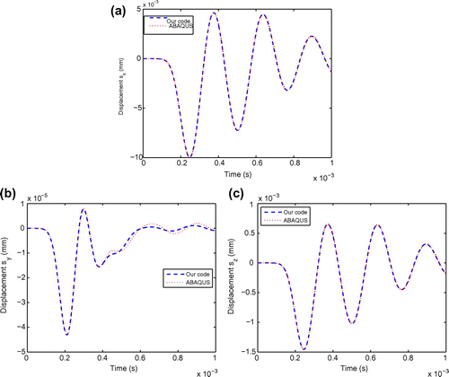
Fig. 4 Distribution of sampling points with the POD–Greedy procedure (a) and the maximum relative RB error of the solution and the output as functions of $N$ (b).

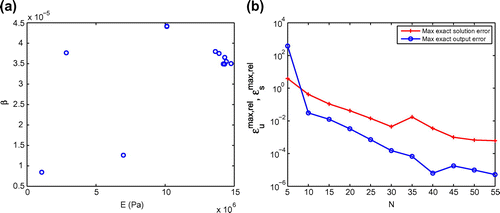
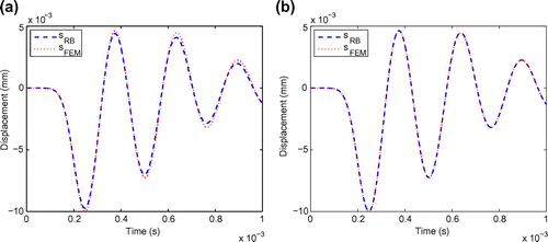
Fig. 5 Comparison of output displacement responses by FEM and RB with ${\mathit{\mu }}_{\mathrm{test}}=(10\times {10}^6\mathrm{Pa},1\times {10}^{-5})$ with $N=2$ (a) and $N=10$ (b) basis functions.

The POD–Greedy algorithm is then implemented to create the RB spaces $Y_N=\{{\mathit{\zeta }}_n,1\le n\le N\},1\le N\le N_{\max }$. The algorithm is actually the POD in the time space and Greedy in the parameter space. We choose $M=5$ (in step (21(21) $$\begin{array}{c}\hfill {\mathit{ϵ}}_u(\mathit{\mu },t^k)=\frac{\parallel e(\mathit{\mu },t^k){\parallel }_Y}{\parallel u_N(\mathit{\mu },t^k){\parallel }_Y};{\mathit{ϵ}}_s(\mathit{\mu },t^k)=\left|\frac{s(\mathit{\mu },t^k)-s_N(\mathit{\mu },t^k)}{s_N(\mathit{\mu },t^k)}\right|,1\le k\le K,\end{array}$$(21) $\mathrm{e}$)) for each Greedy iteration and $N_{\max }=60$ to terminate the iteration procedure4. A sample set ${\mathrm{\Xi }}_{\mathrm{train}}$ is created randomly by a uniform distribution over $\mathcal{D}$ with $n_{\mathrm{train}}=1000$ samples. The distribution of the sample set $S^{\ast }$ is illustrated in Figure 4(a). We show, as a function of $N$: ${\mathit{ϵ}}_u^{\max \mathrm{,}\mathrm{rel}}$ is the maximum over ${\mathrm{\Xi }}_{\mathrm{train}}$ of ${\mathit{ϵ}}_u(\mathit{\mu },t^K)$ and ${\mathit{ϵ}}_s^{\max \mathrm{,}\mathrm{rel}}$ is the maximum over ${\mathrm{\Xi }}_{\mathrm{train}}$ of ${\mathit{ϵ}}_s(\mathit{\mu },t^K)$ in Figure 4(b). The comparison of $s({\mathit{\mu }}_{\mathrm{test}},t)$ vs. $s_N({\mathit{\mu }}_{\mathrm{test}},t)$ for various choices of $N$ are presented in Figure 5, respectively. The numerical results demonstrate that our RB errors are acceptably small, and that the convergence rate is fast for a $N\ll \mathcal{N}$.

Table 2 Comparison of the CPU-time for a FEM, RB and ABAQUS forward analysis.

N	$t_{\mathrm{RB}\mathrm{(}\mathrm{online}\mathrm{)}}$ (s)	$t_{\mathrm{FEM}}$ (s)	$t_{\mathrm{ABAQUS}}$ (s)	$\mathit{\kappa }=t_{\mathrm{FEM}}/t_{\mathrm{RB}\mathrm{(}\mathrm{online}\mathrm{)}}$
10	0.1947	3750	2010	$1.9260\times {10}^4$
20	0.2312	3750	2010	$1.6220\times {10}^4$
30	0.2969	3750	2010	$1.2631\times {10}^4$
40	0.3405	3750	2010	$1.1013\times {10}^4$

All computations were performed on a desktop with processor Intel(R) Core(TM)2 Duo CPU E8200 @2.66GHz 2.66GHz, RAM 3.25GB, 32-bit Operating System. The computation time for the RB forward solver ($t_{\mathrm{RB}\mathrm{(}\mathrm{online}\mathrm{)}}$), the CPU-time for the FEM forward solver by our code ($t_{\mathrm{FEM}}$) and by ABAQUS ($t_{\mathrm{ABAQUS}}$), and the CPU-time saving factor $\mathit{\kappa }=t_{\mathrm{FEM}}/t_{\mathrm{RB}\mathrm{(}\mathrm{online}\mathrm{)}}$ are listed on Table 2, respectively. We observe that while the FEM forward solvers (i.e. our code and ABAQUS) take a thousand of seconds to compute the output displacement responses, the RB solver (with various choices of $N$) takes less than 1 second to find the approximation displacement response with known accuracy. Thus, it is clear that the RB is very efficient and reliable for solving forward problems. Next, our RB model is now ready to be utilized as an efficient forward solver in the inverse analysis.

Inverse procedure

Here, we establish an inverse procedure using our RB model in combination with the Levenberg–Marquardt–Fletcher algorithm to identify rapidly the elastic modulus $E$ and the stiffness Rayleigh damping coefficient $\mathit{\beta }$ of the interfacial tissue in our dental implant-bone structure.

The Levenberg–Marquardt–Fletcher (LMF) algorithm

The considered inverse problem is concerned with the simultaneous estimation of two parameter components: the Young’s modulus $E$ and the stiffness Rayleigh damping coefficient $\mathit{\beta }$ of the interfacial tissue from the ‘measured’ displacement response at the output point (Figure 2(a)). This inverse problem can be regarded as an optimization problem which aims at finding the unknown parameter5${\mathit{\mu }}^{\ast }=(E^{\ast },{\mathit{\beta }}^{\ast })$ that minimizes the following objective function or cost function(28) $$\begin{array}{c}\hfill S(\mathit{\mu })=\sum _{i=1}^K{[s_{N,i}(\mathit{\mu })-s_i^{\mathit{measure}}]}^2=r^{T}r,\end{array}$$(28) where(29) $$\begin{array}{c}\hfill r_i(\mathit{\mu })=s_{N,i}(\mathit{\mu })-s_i^{\mathit{measure}}.\end{array}$$(29) Here, $K$ is the total number of discrete time steps; $s_{N,i}(\mathit{\mu })$ is the ‘computed’ RB displacement response defined in (16(16) $$\begin{array}{c}\hfill W_M=\arg \underset{V_M\subset \mathrm{s}\mathit{pan}\{{\mathit{\xi }}_1,\dots ,{\mathit{\xi }}_{M_{\max }}\}}{\min }(\frac{1}{M_{\max }}\sum _{k=1}^{M_{\max }}\underset{{\underset{¯}{\mathit{\alpha }}}^k\in {\mathbb{R}}^M}{\inf }\parallel {\mathit{\xi }}_k-\sum _{m=1}^M{\mathit{\alpha }}_m^k{v}_m{\parallel }^2).\end{array}$$(16) ) at the time $t_i$ with the parameter $\mathit{\mu }$; $s_i^{\mathrm{measure}}$ is the simulated ‘measured’ displacement response at the time $t_i$ and $\mathit{\mu }=(E,\mathit{\beta })$ is the input material property parameter.

The parameter ${\mathit{\mu }}^{\ast }$ which minimizes the objective function $S$ must satisfy the following set of non-linear algebraic equations:(30) $$\begin{array}{c}\hfill \sum _{i=1}^{K}2\frac{\mathit{\partial }{s}_{N,i}}{\mathit{\partial }{\mathit{\mu }}_j}(s_{N,i}-s_i^{\mathrm{measure}})=2\frac{\mathit{\partial }{\mathit{r}}^{\mathit{T}}}{\mathit{\partial }{\mathit{\mu }}_j}\mathit{r}=2{\mathbf{J}}^T\mathit{r}=0,j=1,2.\end{array}$$(30) The set of equations (34(34) $$\begin{array}{c}\hfill s^{\mathrm{measure}}=s_N({\mathit{\mu }}^{\mathrm{measure}})+\mathit{\omega }\mathit{\sigma },\end{array}$$(34) ) is obtained by differentiating (32(32) $$\begin{array}{c}\hfill |{\mathit{\mu }}_j^{(l+1)}-{\mathit{\mu }}_j^{(l)}|<\mathit{\epsilon },j=1,2,\end{array}$$(32) ) with respect to each component of the parameter $\mathit{\mu }$ and then setting those derivatives equal to zero. The matrix $\mathbf{J}$ is called the Jacobian matrix whose entries are defined as: $J_{\mathit{ij}}=\frac{\mathit{\partial }{r}_i}{\mathit{\partial }{\mathit{\mu }}_j},1\le i\le K,j=1,2$. In order to solve the system (34(34) $$\begin{array}{c}\hfill s^{\mathrm{measure}}=s_N({\mathit{\mu }}^{\mathrm{measure}})+\mathit{\omega }\mathit{\sigma },\end{array}$$(34) ), the Levenberg–Marquardt–Fletcher iterative method [34, 35] is used. The update equation of the parameter $\mathit{\mu }$ at $(l+1)\mathrm{th}$ iteration has the form:(31a) $$\begin{array}{c}\hfill {\mathit{\mu }}^{(l+1)}={\mathit{\mu }}^{(l)}+\mathrm{\Delta }{\mathit{\mu }}^{(l)},\end{array}$$(31a) (31b) $$\begin{array}{c}\hfill \mathrm{\Delta }{\mathit{\mu }}^{(l)}=-({\mathbf{J}}^{{(l)}^T}{\mathbf{J}}^{(l)}+{\mathit{\lambda }}^{(l)}\mathbf{D}{)}^{-1}{\mathbf{J}}^{{(l)}^T}{\mathit{r}}^{\mathbf{(}\mathit{l}\mathbf{)}}.\end{array}$$(31b)

The solution of the inverse problem starts with a suitable guess ${\mathit{\mu }}^{(0)}$, and the iteration procedure is continued until(32) $$\begin{array}{c}\hfill |{\mathit{\mu }}_j^{(l+1)}-{\mathit{\mu }}_j^{(l)}|<\mathit{\epsilon },j=1,2,\end{array}$$(32) where $\mathit{\epsilon }$ is a prescribed tolerance. The entries of the Jacobian matrix $\mathbf{J}$ can be calculated from the following finite difference formula(33) $$\begin{array}{c}\hfill \frac{\mathit{\partial }{r}_i(\mathit{\mu })}{\mathit{\partial }{\mathit{\mu }}_j}\approx \frac{r_i(\mathit{\mu }+\mathit{ϵ}{U}_j)-r_i(\mathit{\mu })}{\mathit{ϵ}},\end{array}$$(33) where $U_j={[{\mathit{\delta }}_{1j},{\mathit{\delta }}_{2j}]}^T$, $\mathit{\delta }$ denotes the Kronecker delta symbol and $\mathit{ϵ}$ is a small number.

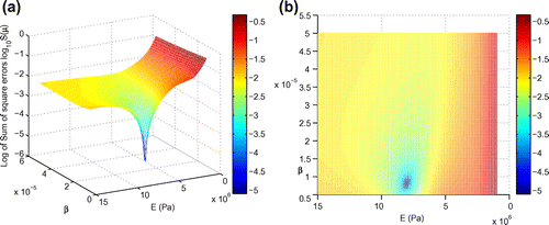
In order to check the uniqueness of solutions of the posed inverse problem, a study on local minima is carried out by plotting the function $S(\mathit{\mu })$ vs. a wide range of both parameter components. Note that we use $N=40$ basis functions in all computations related to our RB model in the inverse analysis (i.e. computations of $s_N(\mathit{\mu })$ in (32(32) $$\begin{array}{c}\hfill |{\mathit{\mu }}_j^{(l+1)}-{\mathit{\mu }}_j^{(l)}|<\mathit{\epsilon },j=1,2,\end{array}$$(32) )). We present on Figure 6 the plot of the logarithm of the function $S(\mathit{\mu })$ vs. both parameter components $E$ and $\mathit{\beta }$ in the parameter domain $\mathcal{D}$. In these plots, we choose ${\mathit{\mu }}^{\mathrm{measure}}\equiv (8\times {10}^6\mathrm{Pa},8\times {10}^{-6})$ for $S(\mathit{\mu })$ as defined in (32(32) $$\begin{array}{c}\hfill |{\mathit{\mu }}_j^{(l+1)}-{\mathit{\mu }}_j^{(l)}|<\mathit{\epsilon },j=1,2,\end{array}$$(32) ). The parameter $\mathit{\mu }$ is taken in the parameter domain $\mathcal{D}$, whereby $\mathcal{D}$ is discretized uniformly into a rectangular grid of $(100\times 100)$ points. The plots confirm that with a particular ${\mathit{\mu }}^{\mathrm{measure}}\equiv (8\times {10}^6\mathrm{Pa},8\times {10}^{-6})$ the function $S(\mathit{\mu })$ has a unique global minimum point which is exactly the ${\mathit{\mu }}^{\mathrm{measure}}$ itself. This also confirms the absence of other local minima (if any) of the function $S(\mathit{\mu })$, and hence ensuring the uniqueness of solutions of our inverse problem.

In the remaining sections, the open-source code [35] with appropriate modifications is used to implement our RB–LMF algorithm.

Numerical results

Effects of $E$ and $\mathit{\beta }$ to output displacement $s_N$

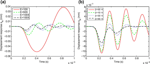
We use $N=40$ basis functions in all computations related to our RB model in this inverse analysis. The effects of both the Young’s modulus $E$ and the stiffness Rayleigh damping coefficient $\mathit{\beta }$ to the displacement response $s_N$ are plotted in Figure 7(a) and (b), respectively. As observed, the Young’s modulus $E$ dominates the width between two consecutive peaks of the displacement response curves (Figure 7(a)), while the coefficient $\mathit{\beta }$ controls the height of these peaks (Figure 7(b)). It is shown that the output displacement responses are very sensitive to these two parameter components.

Fig. 6 Logarithm of the function $S(\mathit{\mu })$ over the parameter domain $\mathcal{D}$ of parameter components $E$ and $\mathit{\beta }$ with (a) an overall 3D view and (b) a xy-view.

Fig. 7 Effects of the Young’s modulus $E$ (with $\mathit{\beta }=1\times {10}^{-5}$) (a) and effects of the stiffness Rayleigh damping coefficient $\mathit{\beta }$ (with $E=10\times {10}^6\mathrm{Pa}$) (b) on displacement responses.

Synthetic data

To verify our RB–LMF procedure, the simulated ‘measured’ displacement responses are used as the input information. A simulated measured displacement response $s^{\mathrm{measure}}$ is generated by adding a Gaussian noise term to the displacement response $s_N({\mathit{\mu }}^{\mathrm{measure}})$ as

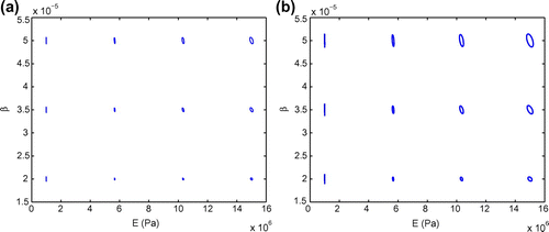
Fig. 8 95% confidence ellipses and computed parameter samples of (a) 100 random tests and (b) 500 random tests.

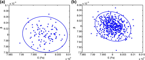
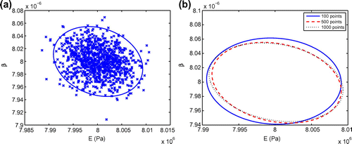
Fig. 9 95% confidence ellipse and computed parameter samples of 1000 random tests (a) and 95% confidence ellipses of all three cases.

Fig. 10 95% confidence ellipses of the sample set $S^{\mathrm{true}}$ with $p_e=1\%$ (a) and $p_e=3\%$ (b) noise added.

Fig. 11 95% confidence ellipses of the sample set $S^{\mathrm{true}}$ with $p_e=5\%$ (a) and $p_e=10\%$ (b) noise added.

(34) $$\begin{array}{c}\hfill s^{\mathrm{measure}}=s_N({\mathit{\mu }}^{\mathrm{measure}})+\mathit{\omega }\mathit{\sigma },\end{array}$$(34) where $\mathit{\omega }$ is a vector which contains random variables with zero mean and unit variance normal [24]; the standard deviation $\mathit{\sigma }$ computed as in [36](35) $$\begin{array}{c}\hfill \mathit{\sigma }=p_e{(\frac{1}{K-1}\sum _{k=1}^K(s_N({\mathit{\mu }}^{\mathrm{measure}},t^k{))}^2)}^{1/2}.\end{array}$$(35) Here, $p_e$ is the noise level (for example, $p_e=0.05$ means a 5% noise level), $K$ is the total number of time steps and $s_N$ is the usual RB displacement response, respectively.

Parameter estimation

As an estimation example, we choose ${\mathit{\mu }}^{\mathrm{measure}}=(8\times {10}^6\mathrm{Pa},8\times {10}^{-6})$ to test our RB–LMF procedure. The lowest value of $\mathit{\mu }\in \mathcal{D}$: ${\mathit{\mu }}^{(0)}=(1\times {10}^6\mathrm{Pa},5\times {10}^{-6})$ is chosen to be the initial guess – which is also independent of ${\mathit{\mu }}^{\mathrm{measure}}$. We first create a number of noisy (or contaminated) outputs $\left\{s^{\mathrm{measure}}\right\}$ as defined in (38(38) $$\begin{array}{cc}\hfill {(\hat{e}(\mathit{\mu },t^k),v)}_Y& =g^{\mathit{eq}}(t^k)f(v)\hfill \\ \hfill & +\sum _{n=1}^N\frac{-u_{Nn}(\mathit{\mu },t^{k+1})+2u_{Nn}(\mathit{\mu },t^k)-u_{Nn}(\mathit{\mu },t^{k-1})}{\mathrm{\Delta }{t}^2}m({\mathit{\zeta }}_n,v)\hfill \\ \hfill & +\sum _{n=1}^N\sum _{q=1}^{Q_c}{\mathrm{\Theta }}_c^q(\mathit{\mu })\frac{-u_{Nn}(\mathit{\mu },t^{k+1})+u_{Nn}(\mathit{\mu },t^{k-1})}{2\mathrm{\Delta }t}{c}^q({\mathit{\zeta }}_n,v)\hfill \\ \hfill & +\sum _{n=1}^N\sum _{q=1}^{Q_a}{\mathrm{\Theta }}_a^q(\mathit{\mu })\frac{-u_{Nn}(\mathit{\mu },t^{k+1})-2u_{Nn}(\mathit{\mu },t^k)-u_{Nn}(\mathit{\mu },t^{k-1})}{4}{a}^q({\mathit{\zeta }}_n,v).\hfill \end{array}$$(38) ), then we use the LMF algorithm to find the corresponding set $\left\{{\mathit{\mu }}^{\mathrm{compute}}\right\}$. This set of computed parameters is then covered by a 95% confidence ellipse which is drawn using the principal components analysis method.[37] For a $p_e=3\%$ noise level, the estimation results which are the 95% confidence ellipses and the computed parameter samples of 100, 500 and 1000 random tests are plotted in Figures 8 and 9(a), respectively. These figures show that the computed parameter samples converge around the center point ${\mathit{\mu }}^{\mathrm{measure}}=(8\times {10}^6\mathrm{Pa},8\times {10}^{-6})$ and that the ellipses’ shapes are nearly similar as the number of random tests increase (Figure 9(b)). Hence, 500 random tests are sufficient to construct reliable 95% confidence ellipses for all test cases afterwards.

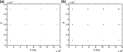
In order to test with many parameters, a sample set $S^{\mathrm{true}}$ of regular $(4\times 3)$ grid pattern over $[1.0\times {10}^6,15\times {10}^6]\mathrm{Pa}\times [2\times {10}^{-5},5\times {10}^{-5}]$ is created. We then implement the RB–LMF procedure with the fixed initial guess ${\mathit{\mu }}^{(0)}=(1\times {10}^6\mathrm{Pa},5\times {10}^{-6})$ and 500 random tests for each true parameter point in the grid. We show the plots of 95% confidence ellipses of each true parameter point with added noise levels $p_e=1\%,3\%,5\%$ and 10% in Figures 10 and 11, respectively. The accuracy and suitability of obtained results show that at lower noise of displacement responses, reliable estimates can be provided by this procedure.

To validate the efficiency of the RB–LMF procedure, total forward solver calls for the RB–LMF inverse analysis are given in Table 3; the total CPU time is recorded and provided in Table 4. It is found that the CPU time of the LMF model using the RB solver6 is significantly faster than the one using the FEM solver. Therefore, the proposed RB–LMF approach strongly reduces the computational time and cost.

Table 3 Total number of forward analyses required in the RB–LMF inverse analysis (for one particular ${\mathit{\mu }}^{\mathrm{measure}}$).

Average number of iterations	Number of RB calls in each iteration	Total RB calls
30	3	$m=90$

Table 4 Comparison of computational time for the LMF model using FEM and RB as forward solvers (for one particular ${\mathit{\mu }}^{\mathrm{measure}}$).

Total RB calls	CPU time for each solver		Total computation time
$m=90$	$t_{\mathrm{FEM}}$	3750 (s)	$m\times t_{\mathrm{FEM}}$	93.75 (h)
	$t_{\mathrm{RB}\mathrm{(}\mathrm{online}\mathrm{)}}$	0.3405 (s)	$m\times t_{\mathrm{RB}\mathrm{(}\mathrm{online}\mathrm{)}}$	35.65 (s)

 

Conclusion

In this paper, a rapid inverse procedure (RB–LMF) is established, which consists of two main stages: constructing a fast elastodynamic RB model and determining inversely material properties via the Levenberg–Marquardt–Fletcher algorithm. We applied the RB–LMF approach to a specific 3D simplified dental implant-bone structure. In the RB stage, the results show that the RB model is very efficient and reliable. In the inverse analysis, the identified results of the RB–LMF approach are very accurate and fast for all test cases: noise-free, contaminated noise, one true parameter, various true parameters. The results of our example support our conclusion that the computational efficiency is greatly increased due to the use of the RB, and that the RB–LMF approach is able to model the non-linear relations between the structural parameters and the non-static responses of complex dental implant structures.

Acknowledgments

This work was supported by the Singapore–MIT Alliance. We thank Dr. Bernard Haasdonk for revising critically the manuscript. We also thank the reviewers for valuable comments which improve the quality of this paper.

Notes

1. This assumption would introduce modelling error and approximation error (due to sharp interfaces) and that functionally graded materials (FGM) would be a more realistic assumption. Since this paper is our first attempt on the development of the RB method for elastic wave equations and its application to the inverse dental implant problem, we consider this simplified 3D model to demonstrate the usefulness of the RB method for certain applications. The FGM assumption approach will be another subject for future work.

2. Generally, for our dental implant problem $u$ and $u^e$ (and hence $s$ and $s^e$) are different due to various environmentally contaminated noise. The simulation treatment of this noise will be described in Section Section34.2.2.

3. In this work, note that we use the Newmark’s scheme $(\mathit{\phi }=\frac{1}{2},\mathit{\psi }=\frac{1}{4})$ as described in Section Section32.2.2.

4. In fact, the POD–Greedy algorithm behaves unstably when $N\ge 60$ basis functions, i.e. the maximum error curves (in Figure 4(b)) will go up with $N\ge 60$. This is because of the high instability of the dual norm of the residual $\parallel R(v;\mathit{\mu },t^k){\parallel }_{Y^{\prime }}$ and the ill conditions of the RB matrices $A_N$ and $C_N$ with larger $N$. However, as observed from Figure 4(b) we already obtain acceptably small RB error even with $N=30$ basis functions and hence, we chose to terminate the procedure with $N_{\max }=60$ basis functions.

5. Here, the vector $\mathit{\mu }$ should be typed in bold as $\mathit{\mu }$, we use the mediumface italic for suitability with previous sections.

6. The work focuses on the real-time context with many online computations, the offline stage is done once and expensive: its computational time is approximately 16 h on the same computer described in Section Section23.5.

Appendix

Calculation of the dual norm of the residual

In this section, we present explicitly the calculation of the dual norm of the residual associated with the discrete RB equation (17(17) $$\begin{array}{cc}\hfill (21\mathrm{a})& \mathrm{Set}{Y}_N=0.\hfill \\ \hfill (21\mathrm{b})& \mathrm{Set}{\mathit{\mu }}^{\ast }={\mathit{\mu }}_0^{\ast }.\hfill \\ \hfill (21\mathrm{c})& \mathrm{While}N\le N_{\max }\hfill \\ \hfill (21\mathrm{d})& \mathcal{W}=\{e_{\mathit{proj}}({\mathit{\mu }}^{\ast },t^k),0\le k\le K\};\hfill \\ \hfill (21\mathrm{e})& Y_{N+M}\leftarrow Y_N⨁\text{POD}(\mathcal{W},M);\hfill \\ \hfill (21\mathrm{f})& N\leftarrow N+M;\hfill \\ \hfill (21\mathrm{g})& {\mathit{\mu }}^{\ast }=\arg \underset{\mathit{\mu }\in {\mathrm{\Xi }}_{\mathit{train}}}{\max }\left\{\frac{\sqrt{\sum _{k=1}^K\parallel R(v;\mathit{\mu },t^k){\parallel }_{Y^{{}^{\prime }}}^2}}{\parallel u_N(\mathit{\mu },t^K){\parallel }_Y}\right\};\hfill \\ \hfill (21\mathrm{h})& S^{\ast }\leftarrow S^{\ast }\bigcup \{{\mathit{\mu }}^{\ast }\};\hfill \\ \hfill (21\mathrm{i})& \mathrm{end}\mathrm{.}\hfill \end{array}$$(17) ) discretized by the Newmark’s scheme $(\mathit{\phi }=\frac{1}{2},\mathit{\psi }=\frac{1}{4})$. We consider the residual defined in (22(22) $$\begin{array}{c}\hfill u_N(\mathit{\mu },t^k)=\sum _{n=1}^N{u}_{Nn}(\mathit{\mu },t^k){\mathit{\zeta }}_n,\forall {\mathit{\zeta }}_n\in Y_N.\end{array}$$(22) ) and its dual norm given in (23(23) $$\begin{array}{cc}\hfill & ({\mathbf{M}}_N+\frac{1}{2}\mathrm{\Delta }t{\mathbf{C}}_N(\mathit{\mu })+\frac{1}{4}\mathrm{\Delta }{t}^2{\mathbf{A}}_N(\mathit{\mu })){\underset{¯}{u}}_N(\mathit{\mu },t^{k+1})\hfill \\ \hfill & =(-{\mathbf{M}}_N+\frac{1}{2}\mathrm{\Delta }t{\mathbf{C}}_N(\mathit{\mu })-\frac{1}{4}\mathrm{\Delta }{t}^2{\mathbf{A}}_N(\mathit{\mu })){\underset{¯}{u}}_N(\mathit{\mu },t^{k-1})\hfill \\ \hfill & +(2{\mathbf{M}}_N-\frac{1}{2}\mathrm{\Delta }{t}^2{\mathbf{A}}_N(\mathit{\mu })){\underset{¯}{u}}_N(\mathit{\mu },t^k)\hfill \\ \hfill & +\mathrm{\Delta }{t}^2{g}^{\mathit{eq}}(t^k){\mathbf{F}}_N,\hfill \\ \hfill & 1\le k\le K-1.\hfill \end{array}$$(23) ). The dual norm of the residual can be computed alternatively as:(36) $$\begin{array}{cc}\hfill \parallel R(v;\mathit{\mu },t^k){\parallel }_{Y^{{}^{\prime }}}& \equiv \underset{v\in Y}{\sup }\frac{R(v;\mathit{\mu },t^k)}{\parallel v{\parallel }_Y},\hfill \\ \hfill & =\parallel \hat{e}(\mathit{\mu },t^k){\parallel }_Y,1\le k\le K-1,\hfill \end{array}$$(36) where $\hat{e}(\mathit{\mu },t^k)\in Y$ is given by the Riesz representation:(37) $$\begin{array}{c}\hfill {(\hat{e}(\mathit{\mu },t^k),v)}_Y=R(v;\mathit{\mu },t^k),\forall v\in Y,1\le k\le K-1.\end{array}$$(37) From (22(22) $$\begin{array}{c}\hfill u_N(\mathit{\mu },t^k)=\sum _{n=1}^N{u}_{Nn}(\mathit{\mu },t^k){\mathit{\zeta }}_n,\forall {\mathit{\zeta }}_n\in Y_N.\end{array}$$(22) ), (26(26) $$\begin{array}{c}\hfill {\mathbf{A}}_{Ni,j}(\mathit{\mu })=\sum _{q=1}^{Q_a}{\mathrm{\Theta }}_a^q(\mathit{\mu }){\mathbf{A}}_{Ni,j}^q,{\mathbf{C}}_{Ni,j}(\mathit{\mu })=\sum _{q=1}^{Q_c}{\mathrm{\Theta }}_c^q(\mathit{\mu }){\mathbf{C}}_{Ni,j}^q,\end{array}$$(26) ) and the affine property (Section310) it thus follows that $\hat{e}(\mathit{\mu },t^k)$ satisfies(38) $$\begin{array}{cc}\hfill {(\hat{e}(\mathit{\mu },t^k),v)}_Y& =g^{\mathit{eq}}(t^k)f(v)\hfill \\ \hfill & +\sum _{n=1}^N\frac{-u_{Nn}(\mathit{\mu },t^{k+1})+2u_{Nn}(\mathit{\mu },t^k)-u_{Nn}(\mathit{\mu },t^{k-1})}{\mathrm{\Delta }{t}^2}m({\mathit{\zeta }}_n,v)\hfill \\ \hfill & +\sum _{n=1}^N\sum _{q=1}^{Q_c}{\mathrm{\Theta }}_c^q(\mathit{\mu })\frac{-u_{Nn}(\mathit{\mu },t^{k+1})+u_{Nn}(\mathit{\mu },t^{k-1})}{2\mathrm{\Delta }t}{c}^q({\mathit{\zeta }}_n,v)\hfill \\ \hfill & +\sum _{n=1}^N\sum _{q=1}^{Q_a}{\mathrm{\Theta }}_a^q(\mathit{\mu })\frac{-u_{Nn}(\mathit{\mu },t^{k+1})-2u_{Nn}(\mathit{\mu },t^k)-u_{Nn}(\mathit{\mu },t^{k-1})}{4}{a}^q({\mathit{\zeta }}_n,v).\hfill \end{array}$$(38) It is clear from linear superposition that we can express $\hat{e}(\mathit{\mu },t^k)$ as:(39) $$\begin{array}{cc}\hfill \hat{e}(\mathit{\mu },t^k)& =g^{\mathit{eq}}(t^k)\mathcal{F}+\sum _{n=1}^N{\mathit{\lambda }}_{m,n}(\mathit{\mu },t^k){\mathcal{M}}_n\hfill \\ \hfill & +\sum _{n=1}^N\sum _{q=1}^{Q_c}{\mathrm{\Theta }}_c^q(\mathit{\mu }){\mathit{\lambda }}_{c,n}(\mathit{\mu },t^k){\mathcal{C}}_{q,n}+\sum _{n=1}^N\sum _{q=1}^{Q_a}{\mathrm{\Theta }}_a^q(\mathit{\mu }){\mathit{\lambda }}_{a,n}(\mathit{\mu },t^k){\mathcal{A}}_{q,n}.\hfill \end{array}$$(39) Here,(40) $$\begin{array}{cc}\hfill {\mathit{\lambda }}_{m,n}(\mathit{\mu },t^k)& =\frac{-u_{Nn}(\mathit{\mu },t^{k+1})+2u_{Nn}(\mathit{\mu },t^k)-u_{Nn}(\mathit{\mu },t^{k-1})}{\mathrm{\Delta }{t}^2},\hfill \\ \hfill {\mathit{\lambda }}_{c,n}(\mathit{\mu },t^k)& =\frac{-u_{Nn}(\mathit{\mu },t^{k+1})+u_{Nn}(\mathit{\mu },t^{k-1})}{2\mathrm{\Delta }t},\hfill \\ \hfill {\mathit{\lambda }}_{a,n}(\mathit{\mu },t^k)& =\frac{-u_{Nn}(\mathit{\mu },t^{k+1})-2u_{Nn}(\mathit{\mu },t^k)-u_{Nn}(\mathit{\mu },t^{k-1})}{4};\hfill \end{array}$$(40) and the parameter-independent terms $\mathcal{F}$, $\mathcal{M}$, $\mathcal{C}$, $\mathcal{A}$ are calculated from:(41) $$\begin{array}{c}\hfill \begin{array}{cccccc}\mathcal{F}\in Y\hfill & \mathrm{from}\hfill & {(\mathcal{F},v)}_Y=f(v),\hfill & \forall v\in Y,\hfill & \hfill & \hfill \\ {\mathcal{M}}_n\in Y\hfill & \mathrm{from}\hfill & {({\mathcal{M}}_n,v)}_Y=m({\mathit{\zeta }}_n,v),\hfill & \forall v\in Y\hfill & \mathrm{for}\hfill & 1\le n\le N,\hfill \\ {\mathcal{C}}_{q,n}\in Y\hfill & \mathrm{from}\hfill & {({\mathcal{C}}_{q,n},v)}_Y=c^q({\mathit{\zeta }}_n,v),\hfill & \forall v\in Y\hfill & \mathrm{for}\hfill & 1\le q\le Q_c,1\le n\le N,\hfill \\ {\mathcal{A}}_{q,n}\in Y\hfill & \mathrm{from}\hfill & {({\mathcal{A}}_{q,n},v)}_Y=a^q({\mathit{\zeta }}_n,v),\hfill & \forall v\in Y\hfill & \mathrm{for}\hfill & 1\le q\le Q_a,1\le n\le N.\hfill \end{array}\end{array}$$(41) From (A1) and (A4) it follows that(42) $$\begin{array}{c}\hfill \begin{array}{cc}\hfill \parallel \hat{e}(\mathit{\mu },t^k){\parallel }_Y^2& \hfill ={(\hat{e}(\mathit{\mu },t^k),\hat{e}(\mathit{\mu },t^k))}_Y\hfill \\ \hfill & \hfill =g^{\mathit{eq}}(t^k)g^{\mathit{eq}}(t^k){\mathrm{\Lambda }}^{\mathit{ff}}\hfill \\ \hfill & \hfill +2\sum _{n=1}^N{g}^{\mathit{eq}}(t^k)\{{\mathit{\lambda }}_{m,n}(\mathit{\mu },t^k){\mathrm{\Lambda }}_n^{\mathit{fm}}+\sum _{q=1}^{Q_c}{\mathrm{\Theta }}_c^q(\mathit{\mu }){\mathit{\lambda }}_{c,n}(\mathit{\mu },t^k){\mathrm{\Lambda }}_{\mathit{qn}}^{\mathit{fc}}\hfill \\ \hfill & \hfill \hfill & +\sum _{q=1}^{Q_a}{\mathrm{\Theta }}_a^q(\mathit{\mu }){\mathit{\lambda }}_{a,n}(\mathit{\mu },t^k){\mathrm{\Lambda }}_{\mathit{qn}}^{\mathit{fa}}\}\hfill \\ \hfill & \hfill +\sum _{n,n^{\prime }=1}^N\{{\mathit{\lambda }}_{m,n}(\mathit{\mu },t^k){\mathit{\lambda }}_{m,n^{\prime }}(\mathit{\mu },t^k){\mathrm{\Lambda }}_{{\mathit{nn}}^{\prime }}^{\mathit{mm}}+2\sum _{q=1}^{Q_c}{\mathrm{\Theta }}_c^q(\mathit{\mu }){\mathit{\lambda }}_{c,n}(\mathit{\mu },t^k){\mathit{\lambda }}_{m,n^{\prime }}(\mathit{\mu },t^k){\mathrm{\Lambda }}_{{\mathit{qnn}}^{\prime }}^{\mathit{mc}}\hfill \\ \hfill & \hfill \hfill & +2\sum _{q=1}^{Q_a}{\mathrm{\Theta }}_a^q(\mathit{\mu }){\mathit{\lambda }}_{a,n}(\mathit{\mu },t^k){\mathit{\lambda }}_{m,n^{\prime }}(\mathit{\mu },t^k){\mathrm{\Lambda }}_{{\mathit{qnn}}^{\prime }}^{\mathit{ma}}\hfill \\ \hfill & \hfill \hfill & +\sum _{q,q^{\prime }=1}^{Q_c}{\mathrm{\Theta }}_c^q(\mathit{\mu }){\mathrm{\Theta }}_c^{q^{\prime }}(\mathit{\mu }){\mathit{\lambda }}_{c,n}(\mathit{\mu },t^k){\mathit{\lambda }}_{c,n^{\prime }}(\mathit{\mu },t^k){\mathrm{\Lambda }}_{{\mathit{qnq}}^{\prime }{n}^{\prime }}^{\mathit{cc}}\hfill \\ \hfill & \hfill \hfill & +2\sum _{q=1}^{Q_c}\sum _{q^{\prime }=1}^{Q_a}{\mathrm{\Theta }}_c^q(\mathit{\mu }){\mathit{\lambda }}_{c,n}(\mathit{\mu },t^k){\mathrm{\Theta }}_a^{q^{\prime }}(\mathit{\mu }){\mathit{\lambda }}_{a,n^{\prime }}(\mathit{\mu },t^k){\mathrm{\Lambda }}_{{\mathit{qnq}}^{\prime }{n}^{\prime }}^{\mathit{ca}}\hfill \\ \hfill & \hfill \hfill & +\sum _{q,q^{\prime }=1}^{Q_a}{\mathrm{\Theta }}_a^q(\mathit{\mu }){\mathit{\lambda }}_{a,n}(\mathit{\mu },t^k){\mathrm{\Theta }}_a^{q^{\prime }}(\mathit{\mu }){\mathit{\lambda }}_{a,n^{\prime }}(\mathit{\mu },t^k){\mathrm{\Lambda }}_{{\mathit{qnq}}^{\prime }{n}^{\prime }}^{\mathit{aa}}\},\hfill \end{array}\end{array}$$(42) where the parameter-independent quantities $\mathrm{\Lambda }$ are defined as(43) $$\begin{array}{c}\hfill \begin{array}{ccc}{\mathrm{\Lambda }}^{\mathit{ff}}\hfill & \hfill ={(\mathcal{F},\mathcal{F})}_Y,\hfill & \hfill \\ {\mathrm{\Lambda }}_n^{\mathit{fm}}\hfill & \hfill ={(\mathcal{F},{\mathcal{M}}_n)}_Y,\hfill & 1\le n\le N,\hfill \\ {\mathrm{\Lambda }}_{\mathit{qn}}^{\mathit{fc}}\hfill & \hfill ={(\mathcal{F},{\mathcal{C}}_{q,n})}_Y,\hfill & 1\le q\le Q_c,1\le n\le N,\hfill \\ {\mathrm{\Lambda }}_{\mathit{qn}}^{\mathit{fa}}\hfill & \hfill ={(\mathcal{F},{\mathcal{A}}_{q,n})}_Y,\hfill & 1\le q\le Q_a,1\le n\le N,\hfill \\ {\mathrm{\Lambda }}_{{\mathit{nn}}^{\prime }}^{\mathit{mm}}\hfill & \hfill ={({\mathcal{M}}_n,{\mathcal{M}}_{n^{\prime }})}_Y,\hfill & 1\le n,n^{\prime }\le N,\hfill \\ {\mathrm{\Lambda }}_{{\mathit{qnn}}^{\prime }}^{\mathit{mc}}\hfill & \hfill ={({\mathcal{M}}_{n^{\prime }},{\mathcal{C}}_{q,n})}_Y,\hfill & 1\le q\le Q_c,1\le n,n^{\prime }\le N,\hfill \\ {\mathrm{\Lambda }}_{{\mathit{qnn}}^{\prime }}^{\mathit{ma}}\hfill & \hfill ={({\mathcal{M}}_{n^{\prime }},{\mathcal{A}}_{q,n})}_Y,\hfill & 1\le q\le Q_a,1\le n,n^{\prime }\le N,\hfill \\ {\mathrm{\Lambda }}_{{\mathit{qnq}}^{\prime }{n}^{\prime }}^{\mathit{cc}}\hfill & \hfill ={({\mathcal{C}}_{q,n},{\mathcal{C}}_{q^{\prime },n^{\prime }})}_Y,\hfill & 1\le q,q^{\prime }\le Q_c,1\le n,n^{\prime }\le N,\hfill \\ {\mathrm{\Lambda }}_{{\mathit{qnq}}^{\prime }{n}^{\prime }}^{\mathit{ca}}\hfill & \hfill ={({\mathcal{C}}_{q,n},{\mathcal{A}}_{q^{\prime },n^{\prime }})}_Y,\hfill & 1\le q\le Q_c,1\le q^{\prime }\le Q_a,1\le n,n^{\prime }\le N,\hfill \\ {\mathrm{\Lambda }}_{{\mathit{qnq}}^{\prime }{n}^{\prime }}^{\mathit{aa}}\hfill & \hfill ={({\mathcal{A}}_{q,n},{\mathcal{A}}_{q^{\prime },n^{\prime }})}_Y,\hfill & 1\le q,q^{\prime }\le Q_a,1\le n,n^{\prime }\le N.\hfill \end{array}\end{array}$$(43)

References

- BranemarkPI, ZarbGA, AlbrektssonT. Tissue-integrated prostheses: osseointegration in clinical dentistry. Chicago (IL): Quintessence; 1985.
- CowinSC. Bone mechanics handbook. Boca Raton (FL): CRC Press; 2001.
- OlivéJ, AparicioC. Periotest method as a measure of osseointegrated oral implant stability. Int. J. Oral Maxillofac. Implants. 1990;5:390–400.
- SwainR, FaulknerG, RaboudJ, WolfaardtJ. A dynamic analytical model for impact evaluation of percutaneous implants. J. Biomech. Eng. 2008;130:13–26.
- Sennerby L, Meredith N. Implant stability measurements using resonance frequency analysis: biological and biomechanical aspects and clinical implications. Periodontology 2000. 2008;47:51–66.
- HuangHM, PanLC, LeeSY, ChiuCL, FanKH, HoKN. Assessing the implant/bone interface by using natural frequency analysis. Oral. Surg. Oral. Med. Oral. Pathol. Oral. Radiol. Endod. 2000;90:285–291.
- Lachmann S, Jäger B, Axmann D, Gomez-Roman G, Groten M, Weber H. Resonance frequency analysis and damping capacity assessment. Part 1: an in vitro study on measurement reliability and a method of comparison in the determination of primary dental implant stability. Clin. Oral Impl. Res. 2006;17:75–79.
- Lachmann S, Jäger B, Axmann D, Gomez-Roman G, Groten M, Weber H. Resonance frequency analysis and damping capacity assessment. Part 2: peri-implant bone loss follow-up. An in vitro study with the PeriotestTM and OsstellTM instruments. Clin. Oral Impl. Res. 2006;17:80–84.
- CapekL, SimunekA, SlezakR, DzanL. Influence of the orientation of the Osstell transducer during measurement of dental implant stability using resonance frequency analysis: a numerical approach. Med. Eng. Phys. 2009;31:764–769.
- Deng B, Han X, Liu GR, Tan KBC. Prediction of elastic properties of the maxillary bone. Proceeding of WCCM VI in conjunction with APCOM’04, Computational Mechanics; 2004.
- DengB, TanKBC, LuY, ZawK, ZhangJ, LiuGR, GengJP. Inverse identification of elastic modulus of dental implant-bone interfacial tissue using neural network and FEA model. Inverse Probl. Sci. Eng. 2009;17:1073–1083.
- ZawK, LiuGR, DengB, TanKBC. Rapid identification of elastic modulus of the interface tissue on dental implants surfaces using reduced-basis method and a neural network. J. Biomech. 2009;42:634–641.
- NataliAN, MeroiEA, WilliamsKR, CalabreseL. Investigation of the integration process of dental implants by means of a numerical analysis of dynamic response. Dent. Mater. 1997;13:325–332.
- DengB, TanKBC, LiuGR. Influence of osseointegration degree and pattern on resonance frequency in the assessment of dental implant stability using finite element analysis. Int. J. Oral Maxillofac. Implants. 2008;23:1082–1088.
- RozzaG, HuynhDBP, PateraAT. Reduced basis approximation and a posteriori error estimation for affinely parametrized elliptic coercive partial differential equations - application to transport and continuum mechanics. Arch. Comput. Methods Eng. 2008;15:229–275.
- HuynhDBP, PateraAT. Reduced basis approximation and a posteriori error estimation for stress intensity factors. Int. J. Numer. Methods Eng. 2007;72:1219–1259.
- Grepl MA, Patera AT. A posteriori error bounds for reduced-basis approximations of parametrized parabolic partial differential equations. ESAIM. Math. Model. Numer. Anal. (M2AN). 2005;39:157–181.
- Tan AYK. Reduced basis methods for 2nd order wave equation: application to one dimensional seismic problem [Master thesis]. Singapore-MIT Alliance, National University of Singapore; 2006.
- NguyenNC, RozzaG, PateraAT. Reduced basis approximation and a posteriori error estimation for the time-dependent viscous Burgers’ equation. Calcolo. 2009;46:157–185.
- VeroyK, PateraAT. Certified real-time solution of the parametrized steady incompressible NavierûStokes equations: rigorous reduced-basis a posteriori error bounds. Int. J. Numer. Methods Fluids. 2005;47:773–788.
- LiuGR, ZawK, WangYY, DengB. A novel reduced-basis method with upper and lower bounds for real-time computation of linear elasticity problems. Comput. Methods Appl. Mech. Eng. 2008;198:269–279.
- LiuGR, LeeJH, PateraAT, YangZL, LamKY. Inverse identification of thermal parameters using reduced-basis method. Comput. Methods Appl. Mech. Eng. 2005;194:3090–3107.
- SawafB, ÖzisikMN, JarnyY. An inverse analysis to estimate linearly temperature dependent thermal conductivity components and heat capacity of an orthotropic medium. Int. J. Heat Mass Transfer. 1995;38:3005–3010.
- TangDW, ArakiN. An inverse analysis to estimate relaxation parameters and thermal diffusivity with a universal heat conduction equation. Int. J. Thermophys. 2000;21:553–561.
- SchnurDS, ZabarasN. An inverse method for determining elastic material properties and a material interface. Int. J. Numer. Methods Eng. 1992;33:2039–2057.
- ZhaoKM, LeeJK. Inverse estimation of material properties for sheet metals. Commun. Numer. Methods Eng. 2004;20:105–118.
- WangS, LiuGR, HoangKC, GuoY. Identifiable range of osseointegration of dental implants through resonance frequency analysis. Med. Eng. Phys. 2010;32:1094–1106.
- HughesTJR. The finite element method: linear static and dynamic finite element analysis. Englewood Cliffs (NJ): Prentice-Hall; 1987.
- DanielWJT. The subcycled Newmark algorithm. Comput. Mech. 1997;20:272–281.
- Patera AT. RB website (augustine); 2007. Available from: http://augustine.mit.edu/methodology.htm
- NguyenNC. A multiscale reduced-basis method for parametrized elliptic partial differential equations with multiple scales. J. Comput. Phys. 2008;227:9807–9822.
- Haasdonk B, Ohlberger M. Reduced basis method for finite volume approximations of parametrized linear evolution equations. ESAIM. Math. Model. Numer. Anal. (M2AN). 2008;42:277–302.
- HuynhDBP, KnezevicDJ, PateraAT. A Laplace transform certified reduced basis method; application to the heat equation and wave equation. C. R. Math. 2011;349:401–405.
- Fletcher R. A modified Marquardt subroutine for nonlinear least squares. Tech. Rep. AERE-R-6799. Harwell (UK): Atomic Energy Research Establishment; 1971.
- Balda M. An algorithm for nonlinear least squares. Institute of Thermomechanics, Academy of Sciences of the Czech Republic, v.v.i., 2010. Available from: http://dsp.vscht.cz/konference_matlab/MATLAB07/prispevky/balda_m/balda_m.pdf
- XuYG, LiuGR. Detection of flaws in composites from scattered elastic-wave field using an improved μGA and a local optimizer. Comput. Methods Appl. Mech. Eng. 2002;191:3929–3946.
- JacksonJE. A User’s Guide to Principal Components. Hoboken (NJ): John Wiley & Sons; 1991.