Application of simulated annealing in a rectangular fin with variable heat transfer coefficient

Abstract

This work deals with the inverse prediction of unknown parameters in a rectangular fin geometry subjected to a variable surface heat transfer coefficient. The unknowns which have been estimated are the thermal conductivity, the heat transfer coefficient at the base of the fin and the exponent for variable heat transfer coefficient. The estimations are done for satisfying a predefined temperature distribution obtained using some known fin properties from a forward method based on the decomposition scheme. Then, using the temperature information only at three locations, through the simulated annealing-based inverse algorithm, the unknowns are estimated. Due to correlated nature of the unknowns, many feasible combinations of the three unknowns have been found, which is proposed to offer the designer flexibility in selecting the fin material. The present inverse algorithm is proposed to be useful in situations where only few discrete temperatures are available, as it helps to find out the possible unknown properties which are required to satisfy a given temperature distribution.

Keywords:

• inverse problem
• thermal conductivity
• variable heat transfer coefficient
• base heat transfer coefficient
• simulated annealing

View correction statement:

Application of simulated annealing in a rectangular fin with variable heat transfer coefficient

1. Introduction

Fins are extended surface used for enhancing the rate of heat transfer.[1] Under a normal situation, along with inside heat conduction, the heat is convected away from its surface, which depends upon the prevailing heat transfer coefficient. The assumption of a constant heat transfer coefficient does not always hold well [2–4]234 as it is found to be dependent on the local temperature. This variation of the heat transfer coefficient with temperature is expressed by a power law expression [4], which increases the non-linearity in the equation governing the energy transport. Using the knowledge of properties, their dependency on the temperature and boundary conditions, the main objective is to obtain the local thermal fields. The method involves solution of a forward/direct problem, which is assumed to be perfect when solved analytically. In this connection, the use of the decomposition method has gained considerable attention for solving heat transfer problems containing enhanced non-linearities [4–7]4567. However, the situation becomes different and more interesting when the final objective in the form of temperature field is only available, but multiple parameters and/or boundary conditions responsible for such field remain unknown. Such cases fall under inverse problems [8], which are mathematically ill posed.

Compared to direct problems, the inverse problems related to fins are relatively new. One of the most important considerations for solving an inverse problem is the proper selection of the optimization tool and a suitable direct/forward algorithm. For problems involving a single unknown with less non-linearity in the governing equation, conventional deterministic optimization methods prove better than the stochastic optimization methods. The details of many optimization algorithms for unknown parameter estimations in fins can be found in archival studies. Huang et al. [9] estimated the conductance in a finned tube heat exchanger using the conjugate gradient method (CGM). Further, the CGM was again used for estimating the heat transfer coefficient in an annular fin by Chen et al. [10]. Das [11] estimated the convective–conductive parameter and the variable conductivity parameter in a rectangular fin using the simplex search method. Recently, Azimi et al. [12] have predicted the base temperature distribution in a non-Fourier fin using Cattaneo-Vernotte model and adjoint CGM. For a cylindrical fin, the application of the simulated annealing (SA) for three parameter estimation was done by Das and Dutta [13]. It is well known that for an objective function which consist of discontinuities and are of multimodal nature, the evolutionary search techniques perform better than the conventional deterministic methods [14]. For the present problem, the inherent difficulties involve the existence of non-linearity (due to variation of heat transfer coefficient) and the existence of multiple and correlated nature of the unknowns. Apart from the SA [13,15]1315, other evolutionary techniques which have been applied to inverse problems are the genetic algorithm [16], the particle swarm algorithm [17], ant colony method [18], etc.

Based on the above discussions, the objective of the present work is to estimate important unknowns in a rectangular fin which are required to satisfy a given temperature distribution. These are the thermal conductivity, k, the exponent for variable heat coefficient, n and the base heat transfer coefficient, h_b. The geometry of the fin is considered to remain fixed. It should be well noted that for a fixed geometry, the convection–conduction parameter, N (which is a non-dimensional quantity) is defined by all three unknowns such as the thermal conductivity, k, the exponent for variable heat coefficient, n and the base heat transfer coefficient, h_b. In the present study, only three temperature locations have been used in the inverse problem for estimating the various unknowns. The required temperature field was obtained by initially solving a direct problem based on the Adomian decomposition method. For optimization purpose, the SA is used due to its various advantages [19–21]192021.

2 Formulation

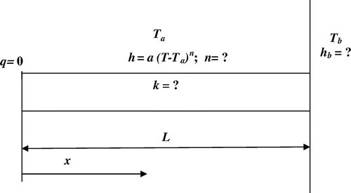
Let us consider a rectangular fin (Figure 1) with insulated tip and the base maintained at a fixed temperature, T_b = 400 K. The ambient temperature is T_a = 300 K. The length, L, the perimeter, p and the areas of cross-section, A, are taken as 0.1 m, 0.012 m and 5 × 10⁻⁴m², respectively. We assume the thermal conductivity, k and the base heat transfer coefficient, h_b to be unknown. In addition to this, we assume the surface heat transfer coefficient to be variable and the relevant exponent, n is also unknown. At steady state, the governing energy equation may be expressed as below [1],(1) $\frac{{\text{d}}^{2}T}{\text{d}{x}^2}-\frac{\mathit{hp}}{\mathit{kA}}(T-T_a)=0$(1)

Figure 1 Geometry of the rectangular fin.

The boundary conditions for the above equation can be expressed as given below,(2) $\begin{array}{c}\hfill x=0\text{;}\frac{\text{d}T}{\text{d}x}=0\hfill \\ \hfill x=L\text{;}T=T_b\hfill \end{array}$(2)

In Equation (1), the heat transfer coefficient, h is assumed to be variable with temperature obeying the following functional relationship [6],(3) $h=a(T-T_a{)}^n$(3)

where, a is a constant. The exponent n represents the type of heat transfer which may cover a wide range from transition boiling (−0.25 < n < −4) to radiation into free space (3 < n < 5) [2–4]234. Therefore, using Equation (3), the governing equation (Equation (1)) takes the following form [4],(4) $\frac{{\text{d}}^{2}T}{\text{d}{x}^2}-\frac{\mathit{ap}}{\mathit{kA}}(T-T_a{)}^{n+1}=0$(4)

For simplicity and generalization, we carry out the non-dimensionalisation in the following manner [4],(5) $\left[\begin{array}{c}\hfill x^{\ast }\hfill \\ \hfill \theta \hfill \\ \hfill N\hfill \end{array}\right]=\left[\begin{array}{c}\hfill x/L\hfill \\ \hfill (T-T_a)/(T_b-T_a)\hfill \\ \hfill {\left(h_b{\mathit{pL}}^2/\mathit{kA}\right)}^{1/2}\hfill \end{array}\right]\text{;}{h}_b=a(T_b-T_a{)}^n$(5)

With the above non-dimensional form (Equation (5)) and after rearrangement of different mathematical terms, the governing equation (Equation (4)) takes the following non-dimensional form [4],(6) $\frac{{\text{d}}^2\theta }{\text{d}{x}^{\ast 2}}-N^2{\theta }^{n+1}=0$(6)

Consequently, the boundary conditions (Equation (2)) also non-dimensionally transforms as below,(7) $\begin{array}{c}\hfill x^{\ast }=0\text{;}\frac{\text{d}\theta }{\text{d}{x}^{\ast }}=0\hfill \\ \hfill x^{\ast }=1\text{;}\theta =1\hfill \end{array}$(7)

Using the above boundary conditions (Equation (7)), the non-dimensional governing equation (Equation (6)) can be either solved analytically or by using any numerical technique such as finite difference method, finite volume method, etc. In this work, it is solved analytically using the Adomian decomposition method which is finding increased popularity for solving mathematical expressions involving increased non-linearities [4–7]4567. Below we discuss the solution procedure.

The governing equation (Equation (6)) can be rewritten as below,(8) $\frac{{\text{d}}^2\theta }{\text{d}{x}^{\ast 2}}=N^2{\theta }^{n+1}$(8)

Using the second-order operator, $L_x=\frac{{\text{d}}^2}{\text{d}{x}^{{\ast }^2}}$ to the above equation, we get the following expression,(9) $L_x\theta =N^2{\theta }^{n+1}$(9)

Next, applying the inverse operator, $L_x^{-1}={\int }_0^{x^{\ast }}{\int }_0^{x^{\ast }}(·)\text{d}{x}^{\ast }\text{d}{x}^{\ast }$ to the above (Equation (9)), and after few mathematical operations, we obtain the components of local temperatures as given below [4–7]4567,(10) $\left[\begin{array}{c}\hfill {\theta }_0\hfill \\ \hfill {\theta }_1\hfill \\ \hfill {\theta }_2\hfill \\ \hfill {\theta }_3\hfill \\ \hfill \cdots \hfill \end{array}\right]=\left[\begin{array}{c}\hfill C\hfill \\ \hfill 1/2C^{1+n}{N}^2{x}^{{\ast }^2}\hfill \\ \hfill 1/24\left(1+n\right)C^{1+2n}{N}^4{x}^{{\ast }^4}\hfill \\ \hfill 1/720\left(1+5n+4n^2\right)C^{1+3n}{N}^6{x}^{{\ast }^6}\hfill \\ \hfill \cdots \hfill \end{array}\right]$(10)

Finally, the local non-dimensional temperature, $\theta$ is obtained by summing all the above components. This can be mathematically represented by the following expression [4–7]4567,(11) $\theta (x^{\ast })=\sum _{i=0}^{\infty }{\theta }_i$(11)

It is worth to note that the unknown constant, C can be easily obtained by the second boundary (right boundary) condition, which is $\theta (1)=1$ and realizing that the non-dimensional temperature, $\theta$ lies in the range 0–1.

The above procedure of calculating temperature, $\theta$ field from using known properties and boundary conditions is termed as the direct (or forward) problem. However, the situation becomes more interesting, when either the exact or a measured thermal field is available, but multiple properties of the system are unknown. Compared to the direct problems, the solutions of such ill-posed inverse problems are relatively difficult because of insufficient mathematical expressions as compared to the number of unknowns. Below, we briefly discuss the formulation of the present inverse problem.

Let us assume an inverse problem where the local temperature, $\theta$ field is available. The temperature, $\theta$ field can be either measured from experiments or calculated using any numerical scheme. For the present analysis, we obtain the temperature, $\theta$ field using the direct method, as mentioned earlier. In the present work, parameters such as the thermal conductivity, k, the exponent for the variable heat coefficient, n and the base heat transfer coefficient, h_b have been assumed to be unknowns. The dimension of the fin is assumed to be already available. Since, three parameters (k, n and h_b) are embedded inside the convective–conductive parameter, N (Equation (5)), thus to solve the inverse problem, we minimize an objective function conventionally described as below [11–13]111213,(12) $\text{Minimize}:\sum _{i=1}^m\{{\theta }_i(N)-{\tilde{\theta }}_i(N){\}}^2$(12)

where, $\tilde{\theta }$ is the available reference or exact field corresponding to some known values of the convection-conduction parameter, $N$. The temperature, $\theta$ field corresponds to some guessed value of the unknowns ($k\text{,}n$ and h_b) to be estimated which are optimized in an iterative manner, and m represents the number of points where the temperature, $\tilde{\theta }$ fields are available. In Equation (12), the available reference or exact, $\tilde{\theta }$ field may contain random measurement errors $(e_r)$. In this work, we induce perturbations between −0.1 and + 0.1, and assumed to follow a Gaussian distribution with approximately zero mean. In connection with the same, the above equation (Equation (12)) gets modified as below [11–13]111213,(13) $\text{Minimize}:\sum _{i=1}^m\{{\theta }_i(N)-[{\tilde{\theta }}_i(N)+e_r]{\}}^2$(13)

where, e_r is the random error as described earlier. In any experiment, it is always desirable to reduce the number of measurement points, m, which for this work may be either thermocouple or any other temperature sensing device. For obtaining the exact temperature, $\tilde{\theta }$ field, we only use three measurement points, two at the boundaries and one at the centre, i.e. m = 3. For updating the guessed temperature, $\theta$ field, the computations must be done for the grid independent situation of measurement points, which in the present work is m = 101. Out of these, three temperatures (${\theta }_1\text{,}{\theta }_{51}\text{,}{\theta }_{101}$) are then fed inside the objective function to compare with the corresponding exact values, $\tilde{\theta }$. Since the inverse algorithm is a combination of the direct method coupled with an optimization algorithm, therefore, the guessed temperature at the centre if updated only on the basis of boundary conditions (and not from its sufficiently close node), it will obviously cause large error. The above exercise, therefore, minimizes the requirement of locating temperature sensing device in real-time experiments. Thus, when the measurements are made at the above three locations, the objective function for temperature field involving no measurement error becomes as expressed below,(14) $\text{Minimize}:({\theta }_1-{\tilde{\theta }}_1{)}^2+({\theta }_{51}-{\tilde{\theta }}_{51}{)}^2+({\theta }_{101}-{\tilde{\theta }}_{101}{)}^2$(14)

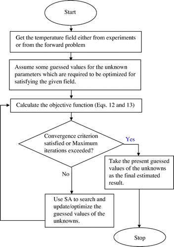
The objective function for the case involving measurement error can also be expressed in the similar manner. The solution procedure of unknown parameter estimation through inverse analysis is shown in Figure 2. For optimization, we have used the SA due to its various advantages [13,15,19–21]1315192021. Below, we provide a brief discussion of the algorithm.

Figure 2 Flowchart of the inverse algorithm.

The SA mimics the annealing process of heat treatment and is based upon the concept of statistical mechanics. During early stages, the concept of the SA was used for studying the atomic behaviour with change in temperature [21]. In the SA, the value of the objective function, J is initially assigned to a higher SA-temperature, $T^{\prime }$ level and successively; it minimizes it to a lower level. Using the initial guess, some random solutions are generated and the differences of the objective functions between the initial guess and the new points (e) are calculated. For a particular new point, if the error, e decreases, then that new point is always accepted with the probability, p = 1. However, if the error, e increases, then the acceptance probability for that point is expressed as below [19–21]192021,(15) $P=\exp \left(\frac{-e}{T^{\prime }}\right)$(15)

The above operation of including worst points is called the uphill approach of the SA [19–21]192021. When all random points are checked, the SA-temperature, $T^{\prime }$ is lowered as below,(16) $T_{k+1}^{\prime }=0.85T_k^{\prime }$(16)

where k is the index for iteration level. The process is repeated and is termed as the re-annealing, which is carried out until the termination criterion is satisfied. For the present study, the termination criterion is taken either when the objective function becomes zero or the SA exceeds a given number of iterations. In this work, 50 iterations have been found to be enough for lowering the objective function to a sufficiently lower value. The following section presents the results and discussions.

3 Results and discussion

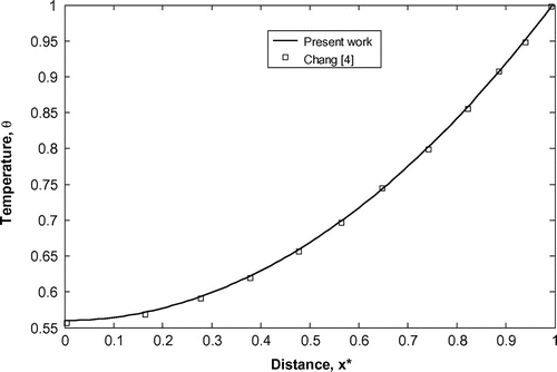
In this section, we present the results of simultaneous estimation of parameters (k, n and h_b) using the knowledge of the temperature, $\theta$ field only at three locations. The required temperature, $\theta$ field is obtained by solving a forward problem based on the Adomian decomposition method. However, before we carry out the optimization study, it is essential to validate the accuracy of the present forward method. Thus, in Figure 3, we compare the steady state temperature, $\theta$ field with the results of Chang [4]. The comparison is shown for the convective–conductive parameter, N = 1 and the exponent for variable heat coefficient, n = −0.75, which is observed to be satisfactory.

Figure 3 Validation of the forward method.

In Table 1, we show the working procedure of the SA algorithm for estimating the unknowns using some arbitrary initial guess as indicated in the table. The results have been done for the case involving exact temperature, $\theta$ field (e_r = 0). The exact values of convective–conductive parameter, N and the exponent for variable heat coefficient, n are 1 and −0.75, respectively. It is well known that all three unknowns, viz. the thermal conductivity, k, the heat transfer coefficient at the base, h_b and the exponent for variable heat transfer coefficient, n are embedded inside the convective–conductive parameter, N. Thus, for a given geometry, so far as the value of the convective–conductive parameter remains the same, the temperature field will also be the same. Using an initial guess, some solutions (10, in the present work) are randomly generated and compared with the objective function of the initial guess. The starting guess for a particular iteration corresponds to the best solution from its previous iteration level. Depending upon the respective value of the objective function and the probability, P (Equation (15)), the selection for the next iteration level is made. In the table, the comparisons have been presented at an initial stage and at a later stage. It can be observed that during later stages, the SA follows a greedy algorithm. This is because during the early stages, many all inferior solutions were accepted. But, during later stages, much improved solutions (Sl. nos. 12–18) were also rejected, thereby allowing more competition amongst the good solutions.

Table 1. Status of solutions during optimization. Range: [k = 20 to 400 W m⁻¹ K¹, n = −1.0 to −0.1 and h_b = 10 to 200 W m⁻² K¹].

Sl. no.	Random points	J	Error difference, e	P = exp (−e/T)	Random no.
Initial guess [k W m^−1 K^1, n, hbW m^−2 K^1] = [95, −0.10, 15]; J = 0.292 during iteration 1; $T^{\prime }$ = 1
1	[57.01, −0.64, 99.0]	0.115	−0.177	Not required	Not required (All are Accepted as error differences, e are negative)
2	[300.26, −0.58, 188.29]	0.230	−0.062
3	[66.14, −0.53, 55.02]	0.209	−0.083
4	[225.85, −0.28, 167.93]	0.230	−0.062
5	[85.76, −0.90, 192.91]	0.054	−0.238
6	[389.11, −0.05, 174.66]	0.265	−0.027
7	[23.56, −0.30, 153.93]	0.026	−0.266
8	[69.71, −0.09, 38.63]	0.254	−0.038
9	[35.59, −0.54, 75.39]	0.093	−0.199
10	[365.22, −0.87, 151.98]	0.246	−0.046
Current guess [kW m^−1 K^1, n, hbW m^−2 K^1] = [34.81, −0.807, 141.08]; J = 2.63 × 10^−8; iteration number = 40. $T^{\prime }$ = 1.8 × 10^−3
11	[29.52, −0.47, 133.81]	1.54 × 10^−4	1.53 × 10^−4	0.918	0.324 < P; Accept
12	[56.61, −0.62, 126.00]	0.078	0.077	1 × 10^−19	0.055 > P; Reject
13	[40.06, −0.08, 199.25]	0.006	0.005	0.062	0.633 > P; Reject
14	[36.22, −0.75, 126.33]	0.008	0.007	0.020	0.170 > P; Reject
15	[27.60, −0.44, 150.17]	0.005	0.005	0.062	0.574 > P; Reject
16	[33.17, −0.84, 112.42]	0.007	0.006	0.035	0.066 > P; Reject
17	[18.54, −0.64, 92.99]	0.006	0.005	0.062	0.754 > P; Reject
18	[22.53, −0.72, 111.36]	0.009	0.008	0.011	0.101 > P; Reject
19	[29.45, −0.48, 137.55]	7.61 × 10^−5	7.60 × 10^−5	0.958	0.270 < P; Accept
20	[72.43, −0.88, 277.76]	1.27 × 10^−4	1.26 × 10^−4	0.932	0.804 < P; Accept

Using the same initial guess as considered in Table 1, in Table 2, we present the comparisons of the exact and the estimated values of the three parameters such as the thermal conductivity, k, base heat transfer coefficient, h_b and the exponent of variable heat coefficient, n. The comparisons have been done both for the case of exact temperature measurements (e_r = 0) as well as for the case involving measurement error (−0.1 ⩽ e_r ⩽  + 0.1) in the temperature field. For each case, the results have been obtained using a different initial guessed value of the parameters. It is observed from Table 2 that there exist many feasible combinations of k, h_b and n which can yield the same temperature, $\theta$ field. However, it is also seen that all feasible combinations yield approximately the same value of the convection–conduction parameters, N. This is due to the fact that for a given geometry (i.e. having fixed length, thickness and area), the local temperature is only a function of the convection–conduction parameter, N and the three unknowns (k, n and h_b) are embedded inside it. In context with the inverse problems, such event is very much useful to a designer, as it offers the flexibility to explore and select the feasible design parameters amongst various possible combinations.

Table 2. Comparison of multiple combinations of unknown parameters (k, n and h_b) satisfying a given temperature field. Range: [k = 20 to 400 W m⁻¹ K¹, n = −1.0 to −0.1 and h_b = 10 to 200 W m⁻² K¹].

Sl. no.	Thermal conductivity, k (W m^−1 K^1)	Variable heat coefficient exponent, n	Base heat transfer coefficient, hb (W m^−2 K^1)	Convective-conductive parameter, N	Measurement error
1	34.81	−0.808	141.08	0.986	er = 0
2	25.68	−0.741	107.45	1.002
3	29.70	−0.264	156.17	1.123
4	60.02	−0.898	199.97	0.894
5	51.12	−0.885	199.58	0.968
6	28.78	−0.419	140.51	1.082	$-0.1⩽e_r⩽+0.1$
7	34.12	−0.151	189.27	1.153
8	43.00	−0.639	188.90	1.026
9	50.60	−0.887	197.33	0.967
10	42.73	−0.576	193.51	1.042

Figure 4 presents the variation of three simultaneously estimated unknowns with iterations of the SA. The comparisons have been shown for temperature, $\theta$ measurements without measurement error (e_r = 0), with measurement points, m = 3 and for the case corresponding to Sl. 1 of Table 2. The exact values of the convective–conductive parameter, N and the exponent for variable heat coefficient, n are taken as 1 and −0.75, respectively. It is observed from Figure 4 that during early stages, the unknowns undergo large fluctuations which become stable after some time. For the present work, 50 iterations of the SA are found to be sufficient, as insignificant updating occurs beyond approximately 40 iterations. In order to show the accuracy of the above estimated values, in Figure 5(a), we present a comparison of the reconstructed and the exact temperature fields. It is observed from the present study that the maximum error difference between the reconstructed and the exact fields is within 0.3% (for measurements with noise) and 0.1% (for measurements without noise). In Figure 5(b), we show the variation of the relevant objective function (Equation (12)), with number of iterations of the SA. It is observed that beyond approximately 40 iterations of the SA, there occurs negligible change in the value of the objective function. The value of the objective function after 50 iterations is found to be $O({10}^{-13})$. After comparing the temperature, $\theta$ field and studying the objective function without any error (e_r = 0), we present these results for the case involving measurement error (−0.1 ⩽ e_r ⩽  + 0.1). In SA, the initial guesses for the unknowns are taken as the same as considered in Sl. 6 of Table 2. The variation of the estimated parameters (k, n and h_b) is shown in Figure 6 and in this case too, 50 iterations of the SA have been found to be sufficient. The details of the measurement error (e_r) are explained earlier. Figure 7 shows the comparisons of the reconstructed temperature, $\theta$ fields and the variation of the relevant objective function (Equation (13)). The results have been found to be similar to the case obtained earlier in Figure 5 and the value of the objective function after 50 iterations is found to be approximately, $O({10}^{-10})$.

Figure 4 Variation of the unknowns with iterations of the SA for temperature, $\theta$ field without measurement error.

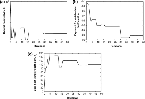
Figure 5 (a) Comparisons of the exact and the reconstructed temperature fields, (b) variation of the objective function; without measurement error (e_r = 0).

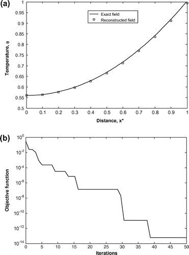
Figure 6 Variation of the unknowns with iterations of the SA for temperature, $\theta$ field; with measurement error.

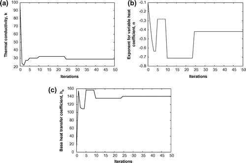
Figure 7 (a) Comparisons of the actual and the reconstructed temperature fields, (b) variation of the objective function; with measurement error (−0.1 ⩽ e_r ⩽ +0.1).

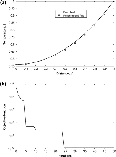
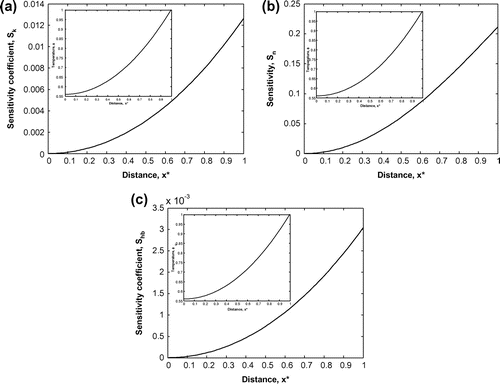
Figure 8 presents the sensitivity coefficients of various parameters estimated in this work. The sensitivity coefficient for any parameter (say k), is defined as $S_k={\left|\left(\frac{\partial \theta }{\partial k}\right)\right|}_{n\text{,}{h}_b}$. Similarly, for other parameters too, the sensitivity coefficients can be represented. For evaluating this, a small change (10⁻³) is made to the relevant parameter (by keeping other parameters fixed) and then the differences of the temperatures, $\theta$ is calculated. Further details about the sensitivity coefficients can be found in [8,22,23]82223. Two important observations can be made from the Figure 8. First, the sensitivity of the exponent for the heat transfer coefficient, S_n is found to be relative more than the other three parameters. In other words, it can be inferred that the temperature, $\theta$ field is more dependent on the value of the exponent for the heat transfer coefficient, S_n. Second, the sensitivity coefficients tend to attain higher values near the hot (east) boundary. This finding is in accordance with the earlier results [11,22]1122, where the temperature field becomes more sensitive to the parameters near the hot boundary as compared to the cold boundary, due to increase in heat loss occurring near the hot boundary.

Figure 8 Comparisons of sensitivity coefficients of the estimated parameters.

4 Conclusions

An inverse problem is solved for estimating parameters such as the thermal conductivity, the exponent for variable heat coefficient and the heat transfer coefficient at the base of the fin. The heat transfer coefficient is assumed to be variable with the temperature. The SA is used to perform the optimization of the relevant objective function. The estimations are done for exact and erroneous temperature field obtained only at three locations. The evolution of the unknown parameters during the optimization process has also been reported. The accuracy of the estimated parameters is benchmarked by comparing the convective–conductive parameter (which contains the three unknowns embedded within itself) and also from the temperature field reconstructions. The feasible combinations of parameters satisfying the same condition have been reported, which is proposed to offer the designer a range of possible alternatives in selecting and various parameters. The present study is concluded to be very useful in finding feasible unknowns by using the knowledge of few discrete temperature data in fins involving variable surface heat transfer coefficient.

Nomenclature

Table

A	area of cross section, m^2
Ai	adomian polynomials
e	error in the SA
er	random measurement error
h	heat transfer coefficient, W m^−2 K^1
k	thermal conductivity, W m^−1 K^1
L	length of the fin, m
m	no. of temperature measurement points
N	convection–conduction parameter
n	exponent for variable heat transfer coefficient
p	perimeter of the fin, m
P	probability of selection in SA
S	sensitivity coefficient
T	temperature, K
$T^{\prime }$	non-dimensional SA temperature level
x	any location along the fin length, m
Greek symbols
$\theta$	non-dimensional temperature
Subscripts
a	ambient
b	fin base
k	index for a particular iteration level of SA
Superscripts
∗	index for non-dimensional distance
∼	exact value

Notes

This article was originally published with errors. This version has been corrected. Please see Corrigendum (http://dx.doi.org/10.1080/17415977.2013.773684)

References

- Kern QD, Kraus DA. Extended surface heat transfer. New York: McGraw-Hill; 1972.
- Liaw SP, Yeh RH. Fins with surface dependent surface heat flux-I: single heat transfer mode. Int. J. Heat Mass Transfer. 1994;37:1509–1515.
- Dul’kin IN, Garas’ko GI. Analytical solutions of 1D heat conduction problem for a single fin with temperature dependent heat transfer coefficient-I: closed-form inverse solution. Int. J. Heat Mass Transfer. 2002;45:1895–1903.
- Chang MH. A decomposition solution for fins with temperature dependent surface heat flux. Int. J. Heat Mass Transfer. 2005;48:1819–1824.
- Kundu B, Bhanja D. An analytical prediction for performance and optimum design analysis of porous fins. Int. J. Refrig. 2011;34:337–352.
- Adomian G. Solving frontier problems in physics: the decomposition method. Dordrecht: Kluwer Academic; 1994.
- Pue-on P, Viriyapong N. Modified Adomian decomposition method for solving particular third-order ordinary differential equations. Appl. Math. Sci. 2012;6:1463–1469.
- Ozisik MN, Orlande HRB. Inverse heat transfer. New York: Taylor and Francis; 2000.
- Huang CH, Wang DM, Chen HM. Prediction of local thermal contact conductance in plate finned-tube heat exchangers. Inverse Probl. Sci. Eng. 1999;7:119–141.
- Chen WL, Yang YC, Lee HL. Inverse problem in determining convection heat transfer coefficient of an annular fin. Energy Convers. Manage. 2007;48:1081–1088.
- Das R. A simplex search method for a conductive-convective fin with variable conductivity. Int. J. Heat Mass Transfer. 2011;54:5001–5009.
- Azimi A, Bamdad K, Ahmadikia H. Inverse hyperbolic heat conduction in fins with arbitrary profiles. Numer. Heat Transfer A. 2012;61:220–240.
- Das R, Dutta PP. Application of simulated annealing for simultaneous estimation of parameters in a cylindrical fin. Numer. Heat Transfer A. 2012;61:699–716.
- De Jong KA. Evolutionary computation: a unified approach. Cambridge, MA: MIT Press; 2006.
- Das R. A simulated annealing-based inverse computational fluid dynamics model for unknown parameter estimation in fluid flow problem. Int. J. Comput. Fluid Dyn. 2012;26:499–513.
- Liu FB. A modified genetic algorithm for solving the inverse heat transfer problem of estimating plan heat source. Int. J. Heat Mass Transfer. 2008;51:3745–3752.
- Chopade RP, Agnihotri E, Singh AK, Kumar A, Uppaluri R, Mishra SC, Mahanta P. Application of a particle swarm algorithm for parameter retrieval in a transient conduction-radiation problem. Numer. Heat Transfer A. 2011;59:672–692.
- Fainekos GE, Giannakoglou KC. Inverse design of airfoils based on a novel formulation of the ant colony optimization method. Inverse Probl. Sci. Eng. 2003;11:21–38.
- Kirkpatrick S, Gelatt CD Jr, Vecchi MP. Optimization by simulated annealing. Science. 1983;220:671–680.
- Rodrigues PPGW, González YM, de Sousa EP, Neto FDM. Evaluation of dispersion parameters for River São Pedro, Brazil, by the simulated annealing method. Inverse Probl. Sci. Eng. 1999. Doi: 10.1080/17415977.2012.665907.
- Metropolis N, Rosenbluth AW, Rosenbluth MN, Teller AH. Equation of state calculations by fast computing machines. J. Chem. Phys. 1953;21:1087–1092.
- Beck JV, Dinwiddie RB. Parameter estimation method for flash thermal diffusivity with two different heat transfer coefficients; Proceedings of 23rd International Thermal Conductivity Conference. Berlin: Springer; 1996.
- Cen H, Lu R, Dolen K. Optimization of inverse algorithm for estimating the optical properties of biological materials using spatially-resolved diffuse reflectance. Inverse Probl. Sci. Eng. 2010;18:853–872.