Identification of space-dependent permeability in nonlinear diffusion equation from interior measurements using wavelet multiscale method

Abstract

Numerical identification of the space-dependent permeability function in a nonlinear diffusion equation is considered. This problem plays an important role in promoting the permeability estimation within multiphase porous media flow. The forward problem is discretized using finite-difference methods and the identification is formulated as a minimization problem with regularization terms. To overcome disturbance of local minimum, a wavelet multiscale method is applied to solve this inverse problem. This method works by decomposing the inverse problem into multiple scales using wavelet transform so that the original inverse problem is reformulated to be a sequence of subinverse problems relying on scale variables, and successively solving these subinverse problems according to the size of scale from the longest to the shortest. The stable and fast regularized Gauss–Newton method is applied to each scale. Numerical simulations show the wide convergence, computational efficiency, anti-noise and de-noising abilities of the proposed algorithm.

Keywords:

• wavelet multiscale method
• inverse problems
• Tikhonov regularization
• nonlinear diffusion equation
• permeability

Introduction

The partial differential equation (PDE) system describing two-phase immiscible flow of incompressible fluids in a porous medium with zero gravity effects is(1.1) $$\begin{array}{cc}\hfill \mathit{\varphi }(\mathbf{x})\frac{\mathit{\partial }S}{\mathit{\partial }t}& -\nabla ·(K(\mathbf{x}){\mathit{\mu }}_w^{-1}(q)k_w(S)\nabla q)=s_w(\mathbf{x},t),\hfill \end{array}$$(1.1) (1.2) $$\begin{array}{cc}\hfill -\mathit{\varphi }(\mathbf{x})\frac{\mathit{\partial }S}{\mathit{\partial }t}& -\nabla ·(K(\mathbf{x}){\mathit{\mu }}_n^{-1}(q)k_n(S)(\nabla q+Q^{\prime }(S)\nabla S))=s_n(\mathbf{x},t),\hfill \end{array}$$(1.2) where $\mathit{\varphi }$ is the porosity, $S$ is the wetting-phase fluid saturation, $K$ is the (absolute) permeability, $\mathit{\mu }$ is the fluid viscosity, $k$ is the relative permeability, $q$ is the wetting-phase fluid pressure, $s$ is the fluid source term and $Q$ is the capillary pressure. The subscripts $w$ and $n$ refer to the wetting and nonwetting fluid phases, respectively, while the prime superscript refers to derivation.

Reservoir simulation based on the above PDE system (and its more detailed versions, including extra physical effects) has the important application value in such fields as oil and gas exploration and management of petroleum reservoirs. With its help, it is easy to select, for example, the type of recovery method, fluid production, injection rates and well locations.

Depending on the independent variables of coefficient functions, the parameter identification based on the above PDE system can be roughly classified in two categories: one is to identify the space-dependent functions $\mathit{\varphi }(\mathbf{x})$ and $K(\mathbf{x})$ and the other one is to identify the saturation-dependent functions $k_w(S)$, $k_n(S)$ and $Q(S)$. This paper is concerned with the research and development of the parameter estimation methodology for one of the space-dependent functions $K(\mathbf{x})$.

There are several modelling and computational difficulties in indentifying the space-dependent permeability function $K(\mathbf{x})$. First, the permeability $K(\mathbf{x})$ is usually modelled as a piecewise constant function, namely, it is defined by a single value within each reservoir simulator grid cell. Therefore, it is interesting to infer as many parameters as there are grid cells in the simulator. This number is frequently more than ${10}^5$ for a field simulation. But, there is far from sufficient information in measurable reservoir quantities such as well pressures and flow rates to identify the permeability function with such a high resolution. This issue is not the subject of this paper, the interested reader is directed to such standard texts as [1–4] for solution. Second, the identification has computational difficulties because the direct model is described by the solution of PDE system that is computationally demanding to solve. Lastly, this inverse problem is highly nonlinear, and fast iterative methods like the quasi-Newton or Gauss–Newton require good initial estimates. When there is no prior information available, the initial value is often chosen to be a constant. However, in oil reservoirs where the permeability usually has very large jumps, the general iterative methods cannot converge when the initial estimate is chosen as an arbitrary constant. So, it is impractical to use them for realistic applications. As stated above, there is a pressing need for parameter identification methods able to solve the later two difficulties. This paper is concentrated on the further development of such parameter identification methods.

A significant amount of literature (see [5–10] and references therein) is devoted to the development of appropriate methods for the identification of $p(\mathbf{x})$ within the linear elliptic equation $-\nabla ·(p(\mathbf{x})\nabla u)=s(\mathbf{x})$, while much less work (e.g. [11–16]) has been done on the parameter identification in the linear parabolic equation $u_t-\nabla ·(p(\mathbf{x})\nabla u)=s(\mathbf{x},t)$.

Both of the above equations can be used for describing the flow processes associated with those described by the PDE system (1.1) and (1.2). The linear elliptic equation is used as the model of single-phase porous media flow with constant fluid density and viscosity, and the linear parabolic equation is used for modelling the slightly compressible flow process of single phase in porous media with constant compressibility, viscosity and porosity. On the basis of above-mentioned basic assumptions, the coefficient function $p(\mathbf{x})$ in actuality is associated with the permeability function by $p(\mathbf{x})=\mathrm{constant}·K(\mathbf{x}\mathrm{)}$. Hence, in the following, $p(\mathbf{x})$ can denote the permeability.

The purpose of this paper is to investigate the numerical identification of the space-dependent permeability function $p(\mathbf{x})$ in the following two-dimensional nonlinear diffusion equations, which is closely relevant to two-phase porous media flow:(1.3) $$\begin{array}{c}\hfill u_t-\nabla ·(p(\mathbf{x})N(u)\nabla u)=s(\mathbf{x},t),(\mathbf{x},t)\in \mathrm{\Omega }\times (0,T),\end{array}$$(1.3) or(1.4) $$\begin{array}{c}\hfill u_t-\nabla ·(p(\mathbf{x})N(\nabla u)\nabla u)=s(\mathbf{x},t),(\mathbf{x},t)\in \mathrm{\Omega }\times (0,T),\end{array}$$(1.4) with the initial-boundary conditions $u(\mathbf{x},0)=u_0(\mathbf{x}),\mathbf{x}\in \mathrm{\Omega }$ and $u(\mathbf{x},t)=0,(\mathbf{x},t)\in \mathit{\partial }\mathrm{\Omega }\times (0,T)$. $s(\mathbf{x},t)$ is a given source term, $N$ is a positive nonlinear function of $u$ or $\nabla u$. For simplicity, $\mathrm{\Omega }$ is assumed to be the unit square, and Equations (1.3) and (1.4) will be written as follows in some places(1.5) $$\begin{array}{c}\hfill u_t-\nabla ·(p(\mathbf{x})N(u,\nabla u)\nabla u)=s(\mathbf{x},t).\end{array}$$(1.5) This identification process is carried out in a manner that the solution $u$ optimally matches the observations $f$ at some fixed points in the spatial domain(1.6) $$\begin{array}{c}\hfill u({\mathbf{x}}^d,t)=f({\mathbf{x}}^d,t),d=1,2,\dots ,D,t\in (0,T).\end{array}$$(1.6) These observations may contain noise.

Inverse coefficient problems for various nonlinear parabolic equations have been investigated by several authors. In [17–19], the authors discuss the numerical identification of parameters in nonlinear convection–diffusion equations. The parameter estimation of a class of nonlinear reaction diffusion equations is studied in [20]. The inverse problem of the parabolic equation with the control parameter is considered in [21]. The parameters of the nonlinear heat conduction problem researched in [22] depend on the space and temperature. The problem studied in [23, 24] coincides with ours, and when the nonlinear function $N=|\nabla u{|}^2$, the problem is the same as the one considered in [25].

As a recently developed inversion strategy, multiscale inversion has a world-wide reputation for speeding up convergence, enhancing stability of inversion, avoiding impact of local minimum and by which we can find the global minimum. The main essence of multiscale inversion is to decompose the original problem into different scales or frequency bands, and to carry out inversion beginning at the longest scale, because the objective function at a longer scale has less local minimum and stronger convexity, so as to have a good opportunity of searching out the global minimum. The global minimum of the longest scale is such a good approximation of the global minimum of the second longest scale that it can be regarded as the initial guess for the second optimization problem. Successively finding upward in this manner can successfully search out the global minimum of the original fine scale problem.

The effectiveness of scale decomposition for the one-dimensional inversion problem was verified in [26]. The multigrid method is a specific form of multiscale methods that can be used to reduce the computational requirements of large-scale numerical problems.[27] This method work by recursively moving between different scales, thereby propagating information between long and short scales. The multigrid method has been primarily used for solving PDEs,[28] but more recently it has been applied to image reconstruction problems such as electrical impedance tomography (EIT) [29] and optical diffusion tomography (ODT).[30] Later, Oh et al. [31, 32] gave the so-called multigrid inversion, which can be employed for the solution of a large variety of inverse problems. The conclusion drawn from these works is that the performance of iterative inversion methods is much better when there exists a scale decomposition.

Wavelet has had many important applications in areas such as signal processing, image analysis and data compression, but its development in applied mathematics is quite recent. The last few years have witnessed the intense activity and interest in the application of wavelet theory and its associated multiresolution analysis.[33] It is very interesting to use wavelet multiresolution to solve inverse problems. More recently, a large amount of literature is devoted to the wavelet multiresolution method for parameter estimation. The wavelet multiresolution method is applied to the parameter identification of an elliptical equation,[34] the parameter identification of two-dimensional acoustic wave equation,[35, 36] the parameter identification of fluid-saturated porous media,[37, 38] the parameter identification of one-dimensional two-phase medium,[39] the multiparameter identification of fluid-saturated porous medium,[40] and the parameter identification of Maxwell equations.[41] All these works testified that wavelet multiresolution is effective for the inverse problems.

This paper attempts to make some further contribution to the permeability estimation within multiphase porous media flow by proposing some practical wavelet multiscale strategies for identifying $p(\mathbf{x})$ in Equation (1.5). The approach is on the basis of the hierarchical approximation of wavelet, and in conjunction with the regularized Gauss–Newton method, which is taken as the basic inversion method applied to each scale. This wavelet multiscale method has been proved to be widely convergent and computationally efficient, and have the anti-noise and de-noising abilities.

In Equation (1.5), the essential nonlinearity, associated with some of the coefficient functions in Equations (1.1) and (1.2), is modelled by the nonlinear function $N(u,\nabla u)$. The nonlinearities, contained in these two coupling equations for $S$ and $q$, are associated with both the dependent variables. $S$ has influence through the actual value of $S$, while $q$ has influence through the value of $\nabla q$. Therefore, Both $u$ and $\nabla u$ are included in the independent variables in $N$.

It is obvious that all aspects of the influence of the nonlinearities in the coefficient functions in Equations (1.1) and (1.2) can be approximately modelled by $N$ rather than entirely. As a result, our purpose should be to evaluate the performance of the above-mentioned wavelet multiscale method when there is a generic nonlinear function multiplying the function to be identified. In addition, the study of Equation (1.5) has cast new light on the information about the performance of the wavelet multiscale method for the PDE system (1.1), (1.2).

The remainder of the paper is arranged as follows. In Section 2, the finite-difference scheme used for discretizing the forward problem is presented. In Section 3, a brief introduction of wavelet and multiresolution analysis is given. In Section 4, the proposed wavelet multiscale method in detail is presented. In Section 5, some numerical simulations are provided. Section 6 consists of a brief summary.

Finite-difference discretization

By using the finite-difference scheme, Equation (1.3) can be discretized as(2.1) $$\begin{array}{c}\hfill \begin{array}{cc}\hfill & \frac{u_{i,j}^n-u_{i,j}^{n-1}}{\mathrm{\Delta }t}-\nabla ·\left(p_{i,j}{N}_{i,j}^n\nabla u_{i,j}^n\right)=s_{i,j}^n,\hfill \\ \hfill & n=1,2,\dots ,M;i=1,2,\dots ,n_1-1;j=1,2,\dots ,n_2-1,\hfill \end{array}\end{array}$$(2.1) where $u_{i,j}^n=u(i\mathrm{\Delta }x,j\mathrm{\Delta }y,n\mathrm{\Delta }t)$, $s_{i,j}^n=s(i\mathrm{\Delta }x,j\mathrm{\Delta }y,n\mathrm{\Delta }t)$, $p_{i,j}=p(i\mathrm{\Delta }x,j\mathrm{\Delta }y)$, $N_{i,j}^n=N(u_{i,j}^n)$, $n_1=\frac{1}{\mathrm{\Delta }x}$, $n_2=\frac{1}{\mathrm{\Delta }y}$, $M=\frac{T}{\mathrm{\Delta }t}$, $\mathrm{\Delta }t$ is the time step length and $\mathrm{\Delta }x$, $\mathrm{\Delta }y$ are the spacings of the rectangular grid in the $x$- and $y$-direction, respectively. $\nabla ·\left(p_{i,j}{N}_{i,j}^n\nabla u_{i,j}^n\right)$ is the discretization of the nonlinear diffusion term; to obtain its expression, the following definitions are given.

The discrete derivatives in the $x$-direction are denoted as$$D_{-}^x{u}_{i,j}^n=\frac{u_{i,j}^n-u_{i-1,j}^n}{\mathrm{\Delta }x},D_{+}^x{u}_{i,j}^n=\frac{u_{i+1,j}^n-u_{i,j}^n}{\mathrm{\Delta }x}$$for the backward and forward difference approximations, respectively. For the discrete derivatives in the $y$-direction, a corresponding notation is used.

The mean values about the discretized permeability $p$ and nonlinear function $N(u)$ can be denoted as$$\begin{array}{cc}\hfill {\overline{p}}_{i,j+\frac{1}{2}}^x& =\frac{1}{2}(p_{i+\frac{1}{2},j+\frac{1}{2}}+p_{i-\frac{1}{2},j+\frac{1}{2}}),{\overline{p}}_{i+\frac{1}{2},j}^y=\frac{1}{2}(p_{i+\frac{1}{2},j+\frac{1}{2}}+p_{i+\frac{1}{2},j-\frac{1}{2}}),\hfill \\ \hfill {\left({\overline{N}}^x\right)}_{i+\frac{1}{2},j}^n& =\frac{1}{2}(N_{i+1,j}^n+N_{i,j}^n),{\left({\overline{N}}^y\right)}_{i,j+\frac{1}{2}}^n=\frac{1}{2}(N_{i,j+1}^n+N_{i,j}^n),\hfill \end{array}$$where $p_{i+\frac{1}{2},j+\frac{1}{2}}=p((i+\frac{1}{2})\mathrm{\Delta }x,(j+\frac{1}{2})\mathrm{\Delta }y)$. The nonlinear diffusion term can then be discretized by$$\nabla ·\left(p_{i,j}{N}_{i,j}^n\nabla u_{i,j}^n\right)=D_{-}^x\left({\overline{p}}_{i+\frac{1}{2},j}^y{\left({\overline{N}}^x\right)}_{i+\frac{1}{2},j}^n{D}_{+}^x{u}_{i,j}^n\right)+D_{-}^y\left({\overline{p}}_{i,j+\frac{1}{2}}^x{\left({\overline{N}}^y\right)}_{i,j+\frac{1}{2}}^n{D}_{+}^y{u}_{i,j}^n\right).$$Because the nonlinear function $N$ is the only difference between Equations (1.3) and (1.4), the finite-difference equation of (1.4) is the same as (2.1), except for $N_{i,j}^n=N(\nabla u_{i,j}^n)$. The mean values about the nonlinear function $N(\nabla u)$ in the $x-$direction are denoted as$$\begin{array}{c},\hfill \\ ({\left({\overline{N}}^x\right)}_{i-\frac{1}{2},j}^n=\frac{1}{2}(\genfrac{}{}{0ex}{}{N{D}_{+}^x{u}_{i,j}^n}{D_{+}^y{u}_{i,j}^n)}+N{D}^{\genfrac{}{}{0ex}{}{(x_{+}{u}_{i-1,j}^n}{D_{+}^y{u}_{i-1,j}^n)}}),\hfill \end{array}$$and a corresponding notation is used for the $y-$direction. As a result, Equation (1.4) can also be approximated by the finite-difference Equation (2.1).

Initial condition and boundary condition are respectively discretized as(2.2) $$\begin{array}{c}\hfill u_{i,j}^0=u_0(i\mathrm{\Delta }x,j\mathrm{\Delta }y),i=0,1,\dots ,n_1;j=0,1,\dots ,n_2,\end{array}$$(2.2) (2.3) $$\begin{array}{c}\hfill \begin{array}{cc}\hfill & u_{0,j}^n=u_{n_1,j}^n=u_{i,0}^n=u_{i,n_2}^n=0,\hfill \\ \hfill & n=1,2,\dots ,M;i=0,1,\dots ,n_1;j=0,1,\dots ,n_2.\hfill \end{array}\end{array}$$(2.3) For the reason of the implicit treatment of the nonlinear diffusion term, the system that needs to be solved for each time level in the forward simulation is nonlinear. We use the Picard iteration to solve these resultant nonlinear systems.

If the nonlinear system is written on the form $B(u)u=b$, where $B(u)$ is a nonsingular matrix depending nonlinearly on $u$, then we iterate$$B(u^{k-1})u^k=b,$$until convergence, with $u^0$ given. $u^0$ is usually the solution from the previous time level. If $N=N(\nabla u)$, this iteration may diverge and a more stabilized three-term version of the Picard iteration is used$$\begin{array}{cc}\hfill & B(u^0)u^1=b,\hfill \\ \hfill & B(\mathit{\beta }{u}^{k-1}+(1-\mathit{\beta })u^{k-2})u^k=b,\mathit{\beta }\in (0.4,0.6),k\ge 2.\hfill \end{array}$$In this paper, the value of $\mathit{\beta }$ is chosen to be 0.5 when this kind of Picard iteration is used.

If we let$$\begin{array}{cc}\hfill u^{\top }& =(u_{1,1}^n,u_{1,2}^n,\dots ,u_{1,n_2-1}^n,u_{2,1}^n,u_{2,2}^n,\dots ,u_{2,n_2-1}^n,\hfill \\ \hfill & \dots ,u_{n_1-1,1}^n,u_{n_1-1,2}^n,\dots ,u_{n_1-1,n_2-1}^n),\hfill \end{array}$$then $B$ is a block tridiagonal matrix. We can conveniently solve this block tridiagonal matrix equations with the chase method. This Picard iteration method is only used to solve the forward problem (2.1).

Remark 1

A natural candidate for the Picard iteration is to linearize Equations (1.3) and (1.4). The identified permeability function $p(\mathbf{x})$ does not depend on $u$ or the gradient $\nabla u$, but on the space variable $\mathbf{x}$. Thus, Equation (1.3), for example, can be linearized into the linear parabolic equation$$v_t-\nabla ·(p(\mathbf{x})\tilde{N}(\mathbf{x},t)\nabla v)=s(\mathbf{x},t),$$where $v(\mathbf{x},t)=u^{(n)}(\mathbf{x},t)$, $\tilde{N}(\mathbf{x},t)=N(u^{(n-1)})$. For this linear parabolic equation, the well-known coefficient identification approaches have been studied in [42, 43].

 

Remark 2

After linearizing, finite-difference discretization (2.1) needs to be applied to the linearized equations, which constitutes another type of forward algorithm. The iteration process for linearization of the nonlinear diffusion Equations (1.3) and (1.4), as is known, may not converge at all. Furthermore, the cases $N=N(u)$ (defined to be as ‘anisotropic nonlinear diffusion’) and $N=N(\nabla u)$ (defined to be as ‘isotropic nonlinear diffusion’) are essentially different cases, in particular, in sense of sufficient conditions for convergence of approximate solutions. The sufficient conditions for the steady state nonlinear operator equation $\mathit{Au}=\nabla ·(N(\nabla u)\nabla u)$ were studied in [44], and the numerical solution of the steady state problem with the nonlinear operator $\mathit{Au}=\nabla ·(N(\nabla u)\nabla u)$ was studied in [45]. The convergence of the forward algorithm adopted in this paper has not been proved in theory; however, the numerical results in Section 5 can show its effectiveness.

 

We can see from the above method that the discretized permeability used in the numerical solution method of the forward problem is $p_{i+\frac{1}{2},j+\frac{1}{2}}$, $i=0,1,\dots ,n_1-1$; $j=0,1,\dots ,n_2-1$. Therefore, the discretized permeability vector $p\in R^{n_1\times n_2}$ is needed.

The initial grid and a coarse grid are, respectively denoted, as ${\mathrm{\Omega }}^{n_1\times n_2}$ and ${\mathrm{\Omega }}^{m_1\times m_2}$, where ${\mathrm{\Omega }}^{m_1\times m_2}$ is got by coarsening ${\mathrm{\Omega }}^{n_1\times n_2}$, $n_1\times n_2$ and $m_1\times m_2$ are, respectively, the grid numbers of the initial grid and the coarse grid. Similar to [24], $p\in R^{m_1\times m_2}$ is defined at ${\mathrm{\Omega }}^{m_1\times m_2}$, and a constant prolongation is used when $p\in R^{n_1\times n_2}$ is needed. The constant prolongation means that the entry of $p$ at ${\mathrm{\Omega }}^{n_1\times n_2}$ is obtained by taking the value from the closed point of ${\mathrm{\Omega }}^{m_1\times m_2}$. In fact, $m_1\times m_2$ is typically dependent on the number of available measurements.

Wavelet multiresolution analysis

In this section, we give a brief introduction of wavelet multiresolution analysis, and refer the interested reader to [33] for more details.

The analysing wavelet $\mathit{\psi }\in L^2(\mathbb{R})$ should satisfy the admissibility condition(3.1) $$\begin{array}{c}\hfill C_{\mathit{\psi }}=2\mathit{\pi }\int d\mathit{\xi }|\mathit{\xi }{|}^{-1}|\hat{\mathit{\psi }}(\mathit{\xi }){|}^2<\infty ,\end{array}$$(3.1) where $\hat{\mathit{\psi }}(\mathit{\xi })$ is the Fourier transform of the wavelet function $\mathit{\psi }(x)$. By dilating and translating, a doubly indexed family of wavelets from $\mathit{\psi }$ can be generated(3.2) $$\begin{array}{c}\hfill {\mathit{\psi }}^{a,b}(x)=|a{|}^{-\frac{1}{2}}\overline{\mathit{\psi }\left(\frac{x-b}{a}\right)}.\end{array}$$(3.2)

Definition 3.1

For any function $f\in L^2(\mathbb{R})$, its continuous wavelet transform with respect to this wavelet family is defined by(3.3) $$\begin{array}{c}\hfill (T^{\mathit{wav}}f)(a,b)=〈f,{\mathit{\psi }}^{a,b}〉=\int \mathit{dxf}(x)·|a{|}^{-\frac{1}{2}}\overline{\mathit{\psi }\left(\frac{x-b}{a}\right)}.\end{array}$$(3.3) Its inverse transform is(3.4) $$\begin{array}{c}\hfill f(x)=C_{\mathit{\psi }}^{-1}{\int }_{-\infty }^{+\infty }{\int }_{-\infty }^{+\infty }\frac{\mathit{dadb}}{a^2}(T^{\mathit{wav}}f)(a,b){\mathit{\psi }}^{a,b}.\end{array}$$(3.4)

 

Definition 3.2

A nest of closed subspaces $\{V_j,j\in \mathbb{Z}\}$ in $L^2(\mathbb{R})$ is said to be a multiresolution analysis (MRA) for $L^2(\mathbb{R})$ if it has the following five properties:

1. $V_j\subset V_{j-1}$, $\forall j\in \mathbb{Z}$;

2. $\bigcap _{j\in \mathbb{Z}}{V}_j=\{0\}$, $\overline{(\bigcup _{j\in \mathbb{Z}}{V}_j)}=L^2(\mathbb{R})$;

3. $f(x)\in V_j\iff f(2^{j}x)\in V_0$, $\forall j\in \mathbb{Z}$;

4. $f(x)\in V_0\iff f(x-k)\in V_0$, $\forall k\in \mathbb{Z}$; and

5. There exists a function $\mathit{\varphi }\in V_0$ such that $\{\mathit{\varphi }(x-k),k\in \mathbb{Z}\}$ is an orthonormal basis in $V_0$.

 

The dilates and translates of the scaling function $\mathit{\varphi }$ comprise the basis function ${\mathit{\varphi }}_{j,k}(x)$ in subspace $V_j$, and the dilates and translates of the wavelet function $\mathit{\psi }$ comprise the basis function ${\mathit{\psi }}_{j,k}(x)$ in subspace $W_j$, which is the orthogonal complement of $V_j$ in $V_{j-1}$. Then, it follows that(3.5) $$\begin{array}{c}\hfill V_0=V_1\oplus W_1=V_2\oplus W_2\oplus W_1=V_J\oplus \underset{j=1}{\overset{J}{⨁}}{W}_j.\end{array}$$(3.5) A given function can be expressed in terms of scaling and wavelet functions(3.6) $$\begin{array}{c}\hfill f=\sum _k{c}_{0,k}{\mathit{\varphi }}_{0,k}(x)=\sum _k{c}_{J,k}{\mathit{\varphi }}_{J,k}(x)+\sum _{j=1}^J\sum _k{d}_{j,k}{\mathit{\psi }}_{j,k}(x).\end{array}$$(3.6) When the problem is decomposed into the $(J+1)$th scale from the $J$th scale, because the space $V_{J+1}$ is merely composed of the lower frequency part of the space $V_J$, the inversed solution in the space $V_{J+1}$ should be an approximation to the original one, which does not contain the higher frequency part. In fact, it is only a local trend near the parameter of the model. However, due to the higher frequency part contained in the subspace $W_{J+1}$ of $V_J$, the information of higher frequency (which cannot be obtained at the longer scale in the space $V_{J+1}$) can be obtained through the inversion in the space $V_J$. The information of further higher frequency, which cannot be obtained in the space $V_J$, can be obtained through the inversion in the space $V_{J-1}$ in the same way. Consequently, the resolution can be gradually enhanced.

Wavelet multiscale method

In this section, we derive a specific wavelet multiscale method for the permeability identification problem of a nonlinear diffusion equation. To deduce this method, we first construct the iteratively regularized Gauss–Newton method as a basic iterative method in Section 4.1, and then design the wavelet multiscale strategy in Section 4.2.

The inversion model and regularized Gauss–Newton method

Equation (1.6) can be discretized as$$u_{{\mathbf{x}}^d}^n=f_{{\mathbf{x}}^d}^n,n=1,2,\dots ,M;d=1,2,\dots ,D.$$The above discretization equation and (2.1)–(2.3) define a vector-valued function $A:P\to F$, where $P$ and $F$ denote vectors, which are composed of $p_{i,j}$ and $f_{{\mathbf{x}}^d}^n$ in the suitable sequence$$P^{\top }=(p_{1,1},p_{1,2},\dots ,p_{1,m_2},p_{2,1},p_{2,2},\dots ,p_{2,m_2},\dots ,p_{m_1,1},p_{m_1,2},\dots ,p_{m_1,m_2}),$$$$F^{\top }=(f_{{\mathbf{x}}^1}^1,f_{{\mathbf{x}}^2}^1,\dots ,f_{{\mathbf{x}}^D}^1,f_{{\mathbf{x}}^1}^2,f_{{\mathbf{x}}^2}^2,\dots ,f_{{\mathbf{x}}^D}^2,\dots ,f_{{\mathbf{x}}^1}^M,f_{{\mathbf{x}}^2}^M,\dots ,f_{{\mathbf{x}}^D}^M).$$Let ${\hat{f}}_{{\mathbf{x}}^d}^n$ denote the observation and forms the vector $\hat{F}$ in the same sequence as $F$,$${\hat{F}}^{\top }=({\hat{f}}_{{\mathbf{x}}^1}^1,{\hat{f}}_{{\mathbf{x}}^2}^1,\dots ,{\hat{f}}_{{\mathbf{x}}^D}^1,{\hat{f}}_{{\mathbf{x}}^1}^2,{\hat{f}}_{{\mathbf{x}}^2}^2,\dots ,{\hat{f}}_{{\mathbf{x}}^D}^2,\dots ,{\hat{f}}_{{\mathbf{x}}^1}^M,{\hat{f}}_{{\mathbf{x}}^2}^M,\dots ,{\hat{f}}_{{\mathbf{x}}^D}^M).$$Then, the problem of inversing $P$ can be transformed into solving the following nonlinear operator equation(4.1) $$\begin{array}{c}\hfill A(P)=\hat{F}.\end{array}$$(4.1) In our numerical simulations, the observation points ${\mathbf{x}}^d$, $d=1,2,\dots ,D$ are on the grid points. The values of $f_{{\mathbf{x}}^d}^n$ will be obtained using a spatial linear interpolation of $u^n$, but if the observation points are not located at the grid points.

For the completeness of the paper, we recall the regularized Gauss–Newton method which is also used in [24]. It is well known that the nonlinear operator Equation (4.1) is an ill-posed problem; therefore, the Tikhonov regularization is introduced. In stead of directly solving (4.1), the optimal problem is considered(4.2) $$\begin{array}{c}\hfill \min \{\parallel A(P)-\hat{F}{\parallel }^2+{\mathit{\alpha }}_1\parallel L_{1}P{\parallel }^2+{\mathit{\alpha }}_2\parallel L_{2}P{\parallel }^2\},\end{array}$$(4.2) where ${\mathit{\alpha }}_1$, ${\mathit{\alpha }}_2$ are the regularization parameters and $L_1$, $L_2$ are the second-order smooth matrices in the $x-$ and $y-$direction, respectively.$$L_{1}P=\left[\begin{array}{c}\hfill 0\hfill \\ \hfill p_{1,1}-2p_{2,1}+p_{3,1}\hfill \\ \hfill p_{2,1}-2p_{3,1}+p_{4,1}\hfill \\ \hfill \cdots \hfill \\ \hfill p_{m_1-2,1}-2p_{m_1-1,1}+p_{m_1,1}\hfill \\ \hfill 0\hfill \\ \hfill 0\hfill \\ \hfill p_{1,2}-2p_{2,2}+p_{3,2}\hfill \\ \hfill p_{2,2}-2p_{3,2}+p_{4,2}\hfill \\ \hfill \cdots \hfill \\ \hfill p_{m_1-2,2}-2p_{m_1-1,2}+p_{m_1,2}\hfill \\ \hfill 0\hfill \\ \hfill \cdots \hfill \\ \hfill 0\hfill \\ \hfill p_{1,m_2}-2p_{2,m_2}+p_{3,m_2}\hfill \\ \hfill p_{2,m_2}-2p_{3,m_2}+p_{4,m_2}\hfill \\ \hfill \cdots \hfill \\ \hfill p_{m_1-2,m_2}-2p_{m_1-1,m_2}+p_{m_1,m_2}\hfill \\ \hfill 0\hfill \end{array}\right],$$$$L_{2}P=\left[\begin{array}{c}\hfill 0\hfill \\ \hfill p_{1,1}-2p_{1,2}+p_{1,3}\hfill \\ \hfill p_{1,2}-2p_{1,3}+p_{1,4}\hfill \\ \hfill \cdots \hfill \\ \hfill p_{1,m_2-2}-2p_{1,m_2-1}+p_{1,m_2}\hfill \\ \hfill 0\hfill \\ \hfill 0\hfill \\ \hfill p_{2,1}-2p_{2,2}+p_{2,3}\hfill \\ \hfill p_{2,2}-2p_{2,3}+p_{2,4}\hfill \\ \hfill \cdots \hfill \\ \hfill p_{2,m_2-2}-2p_{2,m_2-1}+p_{2,m_2}\hfill \\ \hfill 0\hfill \\ \hfill \cdots \hfill \\ \hfill 0\hfill \\ \hfill p_{m_1,1}-2p_{m_1,2}+p_{m_1,3}\hfill \\ \hfill p_{m_1,2}-2p_{m_1,3}+p_{m_1,4}\hfill \\ \hfill \cdots \hfill \\ \hfill p_{m_1,m_2-2}-2p_{m_1,m_2-1}+p_{m_1,m_2}\hfill \\ \hfill 0\hfill \end{array}\right].$$It is easy to know that (4.2) is equivalent to the corresponding normal equation(4.3) $$\begin{array}{c}\hfill A^{\prime }{(P)}^{\top }(A(P)-\hat{F})+{\mathit{\alpha }}_1{L}_1^{\top }{L}_{1}P+{\mathit{\alpha }}_2{L}_2^{\top }{L}_{2}P=0,\end{array}$$(4.3) where the superscript $\top$ is matrix transposition. To avoid the impact of the second derivative, a successive linearization method is used to construct a basic iterative method.

Suppose that the $k$th approximation $P^k$ of Equation (4.3) has already been found. For computing the $(k+1)$th approximation $P^{k+1}$, $A(P)$ is replaced by the linear function $L_k(P)=A^{\prime }(P^k)(P-P^k)+A(P^k)$, and the objective function in (4.2) is replaced by $\parallel L_k(P)-\hat{F}{\parallel }^2+{\mathit{\alpha }}_1\parallel L_{1}P{\parallel }^2+{\mathit{\alpha }}_2\parallel L_{2}P{\parallel }^2$. The corresponding normal equation is(4.4) $$\begin{array}{c}\hfill A^{\prime }{(P^k)}^{\top }[A^{\prime }(P^k)(P-P^k)+A(P^k)-\hat{F}]+{\mathit{\alpha }}_1{L}_1^{\top }{L}_{1}P+{\mathit{\alpha }}_2{L}_2^{\top }{L}_{2}P=0.\end{array}$$(4.4) Use the solution of (4.4) as the $(k+1)$th approximation $P^{k+1}$, then we have(4.5) $$\begin{array}{c}\hfill \begin{array}{cc}\hfill P^{k+1}& =P^k-{[A^{\prime }{(P^k)}^{\top }{A}^{\prime }(P^k)+{\mathit{\alpha }}_1{L}_1^{\top }{L}_1+{\mathit{\alpha }}_2{L}_2^{\top }{L}_2]}^{-1}\hfill \\ \hfill & \times [A^{\prime }{(P^k)}^{\top }(A(P^k)-\hat{F})+{\mathit{\alpha }}_1{L}_1^{\top }{L}_1{P}^k+{\mathit{\alpha }}_2{L}_2^{\top }{L}_2{P}^k],\hfill \\ \hfill & k=0,1,2,\dots \hfill \end{array}\end{array}$$(4.5) This iterative method is the iteratively regularized Gauss–Newton method, which is stable and fast iterative. However, it is as local convergent as the other iterative methods.

Wavelet multiscale method

In theory, the traditional iteration methods such as Newton type are highly effective for the inversion of nonlinear diffusion equation when the initial permeability model is in the neighbourhood of the global minimum of the objective function. But, it has been disappointing to apply directly this inversion technique to real and synthetic data when the initial data is far away from the true data or there is no prior information about permeability available. The fundamental cause of convergence failure lies in the existence of numerous local minimum in the objective function.

The multiscale inversion has an impressive ability to improve the problem about the existence of numerous local minimum because of its decomposition of inverse problem by scale. After the decomposition, the long scale components contain little varying features by reason that at long scales, the number of local minimum is enormously reduced and those that remain are further apart from each other. This leads to the rational statement that ‘the global minimum at a long scale can more easily be searched out than at a short scale by an iterative descent method’. The global minimum of the longest scale component is such a good approximation of the global minimum of the second longest scale component that it can be regarded as the initial guess of the second optimization problem. Thus, the solution obtained from the longest scale component is then recursively refined in this manner.

This thesis makes an attempt to use wavelet to implement decompositions, and to take the regularized Gauss–Newton method as the basic inversion method at each scale. This inversion procedure, named by the wavelet multiscale method, provides several unique advantages over the other multiscale approaches such as coarse-to-fine approaches and multigrid algorithms. First, it can greatly reduce computation since the objective function at a longer scale has less local minimum and stronger convexity. Second, it possesses widely convergent region as the regularized Gauss–Newton method cannot easily immerge in partial minimum at a long scale. Third, the inversion result can be improved when the data is strongly noisy because wavelet has good de-noising performance. Therefore, it is more effective to apply this procedure to the inverse problem.

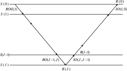
As illustrated in Figure 1, there are three elements required for the wavelet multiscale method. The first one is the restriction operator which maps the original problem to longer scales, the second one is the relaxation operator which performs relaxation at each scale and the last one is the injection operator by which the solution available at a longer scale is injected back up to a shorter scale. In Figure 1, $S(0)$ represents the scale 0 on which the original problem is defined. The restriction operator $\mathit{RO}(0,1)$ which restricts the original problem from $S(0)$ to $S(1)$ is selected as the wavelet decomposition algorithm

Fig. 1 Description of the wavelet multiscale inversion algorithm.

(4.6) $$\begin{array}{c}\hfill \mathit{RO}(0,1):S(0)\to S(1).\end{array}$$(4.6) Once the problem has been restricted to the longer scale $S(1)$, the solution at this scale is obtained by the relaxation operator $R(1)$. In this paper, we use the regularized Gauss–Newton method as the relaxation operator. Once the relaxation operator has been used to solve the component of the problem at scale $S(1)$, the solution is then injected back up to the scale $S(0)$ with the injection operator $\mathit{IO}(1,0)$, which is chosen to be wavelet reconstruction algorithm(4.7) $$\begin{array}{c}\hfill \mathit{IO}(0,1):S(1)\to S(0).\end{array}$$(4.7) The parts of the problem that were not resolved at scale $S(1)$ are solved by the relaxation operator $R(0)$. This completes the description of the two-scale wavelet multiscale solution for nonlinear problem. The multiscale wavelet inversion method can be easily got by replacing the relaxation operator $R(1)$ with another two-scale wavelet multiscale solution recursively, which is also shown in Figure 1.

The object to be decomposed may be the permeability model, the wave field, the source, or a combination of the three. There are two basic methods to carry out the decomposition. The first method is to make wavelet transform on all the permeability, the wave field and the source. The increase in the scale leads to the drastic reduction in the dimension of the discrete inverse problem, especially for high-dimensional continuous problems. However, the difficulties that confront us are that the treatment on the boundary and the direct wave is bothersome, and the high precision of forward calculation is demanded. The second method is to make wavelet transformation only on the wave field and the source.

The second method is chosen in this article because it is very simple, and does not need the high precision of forward calculation. The wave field and source are transformed by wavelets into different scales. The initial nonlinear minimum problem is then accordingly decomposed into a sequence of nonlinear minimum problems at different scales. As a matter of fact, the multiscale decomposition is an inversion strategy, and we can combine it with any iterative method to construct effective inversion method. Based on the multiscale decomposition, the regularized Gauss–Newton method is executed at the longest scale $S(J)$ until an approximation $P_J^{\ast }$ is found at this scale. Then, use same procedure as above at the second longest scale using $P_J^{\ast }$ as the initial guess. Successively finding upward in this manner can successfully search out the global minimum of the original fine scale problem. 

Numerical simulations

Numerical simulations are presented here to assess the performance of the proposed method, and carried out using MATLAB 7.0.

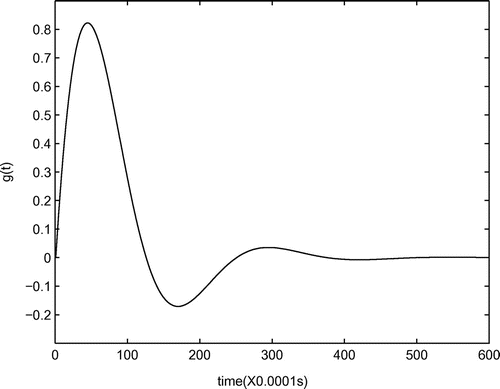
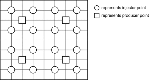
We set $\mathrm{\Omega }=[0,1]\times [0,1]$, $u_0(\mathbf{x})=0$, $T=0.06$ and $M=30$. The source function is$$s(\mathbf{x},t)=g(t)[\sum _{i=1}^{16}\mathit{\delta }(\mathbf{x}-{\mathbf{x}}^i)-4\sum _{p=1}^4\mathit{\delta }(\mathbf{x}-{\mathbf{x}}^p)],$$where $g(t)$ is shown in Figure 2, $\mathit{\delta }(·)$ is the Dirac delta, the coordinates of the producer points ${\mathbf{x}}^q$ for $q=1,\dots ,4$, are $(\frac{1}{4},\frac{1}{4})$, $(\frac{1}{4},\frac{3}{4})$, $(\frac{3}{4},\frac{1}{4})$ and $(\frac{3}{4},\frac{3}{4})$, respectively. There are four injector points around every producer point. Figure 3 shows the locations of producer points ${\mathbf{x}}^q$, $q=1,\dots ,4$, and injector points ${\mathbf{x}}^i$, $i=1,\dots ,16$. We place 16 receivers in each injector point simultaneously, that is $D=16$. In all examples, the grid cell size of ${\mathrm{\Omega }}^{m_1\times m_2}$ is $(2\mathrm{\Delta }x,2\mathrm{\Delta }y)$, which means $m_1=\frac{n_1}{2}$, $m_2=\frac{n_2}{2}$.

Fig. 2 The function $g(t)$.

Fig. 3 Simulation geometry with the locations of producer points and injector points.

For the exact data ${\hat{f}}_{{\mathbf{x}}^d}^n$, its noisy version is(5.1) $$\begin{array}{c}\hfill {\left({\hat{f}}_{{\mathbf{x}}^d}^n\right)}^{\mathit{\sigma }}=(1+\mathit{\sigma }·{\mathit{\eta }}_d^n){\hat{f}}_{{\mathbf{x}}^d}^n,\end{array}$$(5.1) where $\{{\mathit{\eta }}_d^n\}$, $d=1,2,\dots ,D$; $n=1,2,\dots ,M$, are generated by the function randn$(D\times M,1)$ in Matlab (randn$(D\times M,1)$ generates a $(D\times M)$-dimension vector with random components, chosen from a normal distribution with mean zero, variance one and standard deviation one). $\mathit{\sigma }$ is referred to as the noise level.

Table 1 The iteration numbers when the parameters converge to the real value by WM6, WM3 and RGN.

Number	Initial value	WM6	WM3	RGN
1	2.05	8	5	8
2	2.15	8	6	9
3	2.25	8	7	10
4	2.35	8	8	No convergence
5	2.45	8	10	No convergence
6	2.55	10	No convergence	No convergence

Fig. 4 The solution of the forward problem after 30 time steps, i.e. $u^{30}$.

Fig. 5 The true model and inversion results with the noise level $\mathit{\sigma }={10}^{-2}$ in Example 5.2: (a) is the true model; (b) is the inversion result for $N(u)$; and (c) is the inversion result for $N(\nabla u)$.

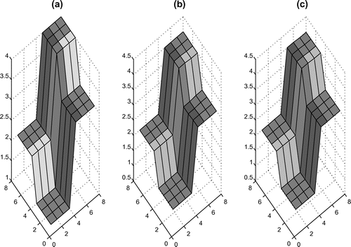
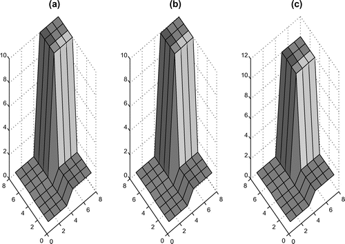
Fig. 6 The true model and inversion results with the noise level $\mathit{\sigma }={10}^{-2}$ in Example 5.3: (a) is the true model; (b) is the inversion result for $N(u)$; and (c) is the inversion result for $N(\nabla u)$.

Fig. 7 The relative $l^2$ errors with respect to different number $D$ with the noise level $\mathit{\sigma }={10}^{-3}$ in Example 5.4.

Fig. 8 The relative $l^2$ errors with respect to different number $D$ with the noise level $\mathit{\sigma }={10}^{-2}$ in Example 5.4.

Fig. 9 The relative $l^2$ errors with respect to different number $D$ with the noise level $\mathit{\sigma }={10}^{-1}$ in Example 5.4.

Fig. 10 The true model in Example 5.5.

Fig. 11 The inversion result at the original scale with the noise level $\mathit{\sigma }={10}^{-2}$ in Example 5.5.

Fig. 12 The true model in Example 5.6.

Fig. 13 The inversion result at the original scale with the noise level $\mathit{\sigma }={10}^{-2}$ in Example 5.6.

Fig. 14 The true model in Example 5.7.

Fig. 15 The inversion results at different scales with the noise level $\mathit{\sigma }=4\times {10}^{-2}$ in Example 5.7.

In the first four examples, $\mathrm{\Delta }x=\mathrm{\Delta }y=\frac{1}{8}$ and the true permeability, $p(\mathbf{x})$, is piecewise constant(5.2) $$\begin{array}{c}\hfill p(\mathbf{x})=\{\begin{array}{cc}{p}_1^c,\hfill & \mathbf{x}\in [0,0.5]\times [0,0.5],\hfill \\ p_2^c,\hfill & \mathbf{x}\in [0,0.5]\times [0.5,1],\hfill \\ p_3^c,\hfill & \mathbf{x}\in [0.5,1]\times [0,0.5],\hfill \\ p_4^c,\hfill & \mathbf{x}\in [0.5,1]\times [0.5,1],\hfill \end{array}\end{array}$$(5.2) where $p_i^c=i$, $i=1,\dots ,4$, unless otherwise mentioned. Because of the relatively small dimension, the regularization parameters can be chosen as ${\mathit{\alpha }}_1={\mathit{\alpha }}_2=0$. In the last three examples, $\mathrm{\Delta }x=\mathrm{\Delta }y=\frac{1}{16}$, the complex permeability models and regularization parameters will specifically be described in the each example.

The longest scale $J$ of wavelet decomposition is 3 in all examples except for Example 5.1. The iteratively regularized Gauss–Newton method (4.5) will be terminated when the stopping condition $\parallel P^{k+1}-P^k\parallel \le {10}^{-4}$ is fulfilled.

Example 5.1

In the first example, we, respectively, use the the wavelet multiscale method with $J=6$ (WM6), wavelet multiscale method with $J=3$ (WM3) and iteratively regularized Gauss–Newton method (RGN). The nonlinear function $N$ is $N(u)=u^2+u+1$ and $\mathit{\sigma }=0$. The initial estimate $P^0$ is chosen to be a constant. To compare differences among these methods, the iteration numbers when the parameters converge to the real value are compiled in Table 1.

 

We first compare WM3 with RGN. Looking at Table 1, from experiments 1, 2 and 3, one can see that the wavelet multiscale procedure is more efficient than the iteratively regularized Gauss–Newton method. Moreover, from experiments 4 and 5, one observed that the iteratively regularized Gauss–Newton method does not converge to the real value when the initial estimate is poor, while for the wavelet multiscale procedure, convergence can be achieved. Then, WM6 is compared with WM3 and RGN. It can be seen from experiment 6 that as the scale of the wavelet multiscale procedure is increased, its convergence region gets wider. In addition, experiments 1–5 show that when the initial value is around the real value, the increase in the scale leads to the increase in the calculation amount; however, when the initial value is far away from the real value, the increase in the scale can lead to the decrease in the calculation amount. As a whole, it is concluded that the wavelet multiscale method is widely convergent and efficient.

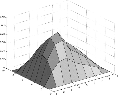
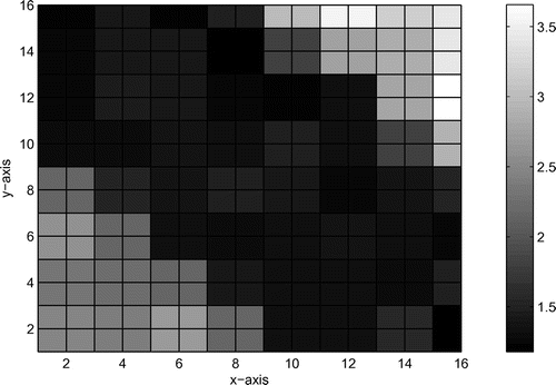
For the sake of validating the effectiveness of the forward algorithm, forward numerical simulation using the model in Example 5.1 is carried out. Only here, we let $u_0(\mathbf{x})=\sin (\mathit{\pi }x)\sin (\mathit{\pi }y)$ and $g(t)=0$, to ensure that all the parameters are the same as those in [47]. Figure 4 shows the solution $u$ of the forward problem, in the last time level, i.e. $u(T)$. This numerical result, which is in agreement with reference [47] for equivalent parameters, proves correctness and effectiveness of the forward algorithm. Forward numerical simulations using the various models in the following examples are also carried out, and we find that they all illustrate its effectiveness. But since this issue is not what this paper is about, we do not list these numerical results of the forward algorithm.

Example 5.2

In this example, we only use Algorithm 1. The nonlinear functions $N$ are, respectively, chosen as $N(u)=u^4+u^3+u^2+u+1$ and $N(\nabla u)=1+0.1|\nabla u{|}^2$. Choose $P^0\equiv 2.5$, $\mathit{\sigma }={10}^{-2}$. Figure 5 shows the inversion results, and the relative $l^2$ errors for $N(u)$ and $N(\nabla u)$ are approximately equal to 0.0030 and 0.0021, respectively.

 

Example 5.3

In oil reservoirs, the permeability usually has greatly large jumps; therefore, let $p_i^c={10}^{i-3}$, $i=1,\dots ,4$. In this example, we also use Algorithm 1. The nonlinear functions $N$ are, respectively, chosen to be $N(u)=u^4-u^3+u^2-u+1$ and $N(\nabla u)=\frac{1}{1-0.1|\nabla u{|}^2}$. Choose $P^0\equiv 0.1$, $\mathit{\sigma }={10}^{-2}$. Figure 6 shows the inversion results, and the relative $l^2$ errors for $N(u)$ and $N(\nabla u)$ are approximately equal to 0.0042 and 0.0031, respectively.

 

From these two examples, we can see that the wavelet multiscale method is effective for the different $N-$functions, even if $N$ is highly nonlinear. Furthermore, in Example 5.3, the iteratively regularized Gauss–Newton method is not convergent when the initial estimate is chosen as an arbitrary constant. Thus, it is easily concluded that the wavelet multiscale procedure is effective and even necessary in oil reservoir simulation.

Example 5.4

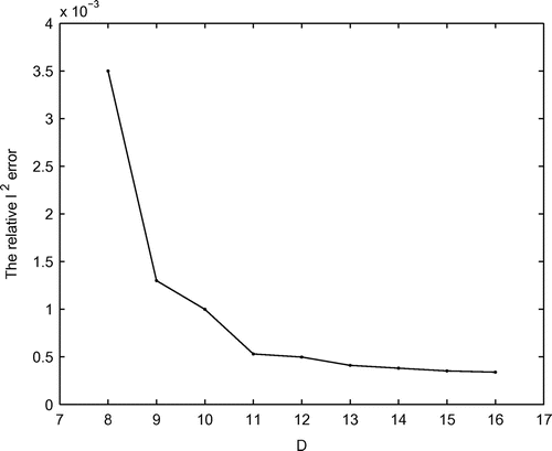
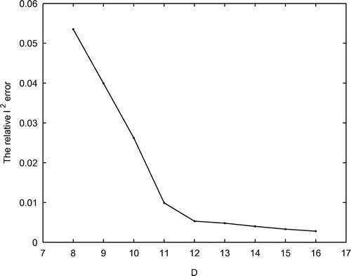
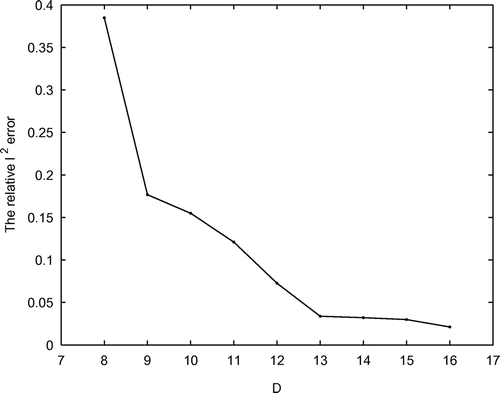
The stability and accuracy of numerical solutions of the considered inverse problems should depend on the number $D$ of the receivers. Hence, we reduce the number $D$ gradually, and the receivers are randomly removed. In this example, we also use Algorithm 1. Choose $N(u)=u^2+u+1$, $P^0\equiv 2.5$. Figures 7, 8 and 9 plot the relative $l^2$ errors vs. different number $D$ for $\mathit{\sigma }={10}^{-3}$, $\mathit{\sigma }={10}^{-2}$ and $\mathit{\sigma }={10}^{-1}$, respectively.

 

From this example, we can see that the number $D$ of the receivers plays an important role in the reconstructed results. As the number $D$ of the receivers increased, the quality of the results improved greatly. That is, the increase in the number $D$ leads to the improvements in the stability and accuracy of numerical solutions.

Example 5.5

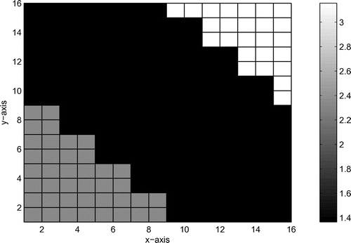
In this example, we consider an oblique-stratified medium containing two interfaces, which is depicted in Figure 10. Choose $N(u)=u^3+u^2+u+1$, $P^0\equiv 2$, $\mathit{\sigma }={10}^{-2}$ and ${\mathit{\alpha }}_1={\mathit{\alpha }}_2={10}^{-11}$. Figure 11 shows the inversion result at scale 0. Starting from the same initial estimate, RGN is also convergent, but takes about 133.47% CPU time of the wavelet multiscale method.

 

Example 5.6

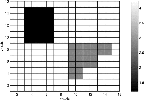
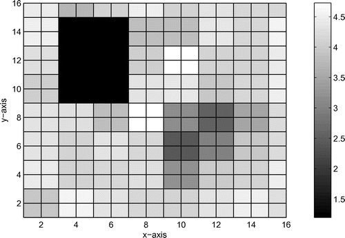
In this example, we consider the model of two anomalous bodies in a homogeneous medium with a permeability of 4.25. The anomalous bodies have the permeability of 1.18 and 2.79, respectively. Choose $N(u)=3u^2+2u+1$, $P^0\equiv 4$, $\mathit{\sigma }={10}^{-2}$ and ${\mathit{\alpha }}_1={\mathit{\alpha }}_2={10}^{-13}$. Figures 12 and 13 show this model and its inversion result at scale 0, respectively. Starting from the same initial estimate, RGN is not convergent.

 

Example 5.7

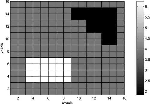
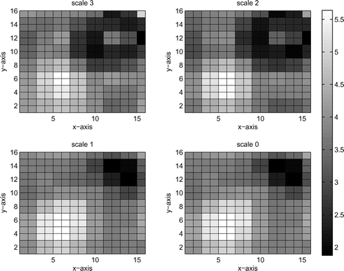
In this example, we consider another model of two anomalous bodies in a homogeneous medium with a permeability of 3.85. The anomalous bodies have the permeability of 1.79 and 6.28, respectively. Choose $N(u)=u^2+u+1$, $P^0\equiv 3$, $\mathit{\sigma }=4\times {10}^{-2}$ and ${\mathit{\alpha }}_1={\mathit{\alpha }}_2={10}^{-11}$. Figures 14 and 15 show this model and its inversion results at different scales, respectively. The relative $l^2$ errors for the inversion results at every scale from the longest scale to the shortest scale are approximately equal to 0.1513, 0.1368, 0.1039 and 0.1054, respectively.

 

Based on the numerical results in Examples 5.5–5.7, we conclude that the merits of the wavelet multiscale method, such as the wide convergence, computational efficiency and anti-noise ability, still exist for the large-scale and complicated model. Furthermore, in Example 5.7, the inversion result at scale 1 is better than the one at scale 0. Thus, it is easily concluded that the wavelet multiscale procedure can eliminate noise to a certain degree when the data is strongly noisy. The reason for this is probably that wavelet has good de-noising performance.

Conclusion

This paper successfully designs a wavelet multiscale method for the parameter identification of a nonlinear diffusion equation, and numerical simulations show its widely convergence, computationally efficiency, anti-noise and de-noising abilities. Furthermore, this new method is effective for the highly nonlinear $N$-functions, and even necessary in oil reservoir simulation for the greatly large jumps in the permeability. In fact, the wavelet multiscale method is general and can be easily generalized to the other kinds of inverse problems, especially the permeability identification problems in the multiphase porous media flow equations.

Acknowledgments

The authors are grateful to anonymous referees for their valuable comments. The authors would like to thank Laura Huxley and the typesetting team for their kind help. This work was supported by the National Natural Science Foundation of China (11101109, 11271102) and the Natural Science Foundation of Hei-long-jiang Province of China (A201107).

References

- Shah PC, Gavalas GR, Seinfeld JH. Error analysis in history matching, the optimum level of parameterization. Soc. Pet. Eng. J. 1978;6:219–228.
- Reynolds AC, He N, Chu L, Oliver D. Reparameterization techniques for generating reservoir descriptions conditioned to variograms and well-test pressure data, SPE 30588. USA: Dallas. Proceedings of the SPE Annual Technical Conference and Exhibition; 1995.
- Cuypers M, Dubrule O, Lamy P, Bissell R. Optimal choice of inversion parameters for history matching with the pilot point method. Proceedings of the 6th European Conference on the Mathematics of Oil Recovery. UK: Peebles; 1998.
- Grimstad AA, Mannseth T, Nordtvedt JE, Nævdal G. Reservoir characterization through scale splitting. Proceedings of the 7th European Conference on the Mathematics of Oil Recovery, Baveno, Italy; 2000.
- Chen Z, Zou J. An augmented Lagrangian method for identifying discontinuous parameters in elliptic systems. SIAM J. Control Optim. 1999;37:892–910.
- Knowles I. Parameter identification for elliptic problems. J. Comput. Appl. Math. 2001;131: 175–194.
- Chan TF, Tai XC. Level set and total variation regularization for elliptic inverse problems with discontinuous coefficients. J. Comput. Phys. 2003;193:40–66.
- Gockenbach MS, Khan AA. An abstract framework for elliptic inverse problems: part 1. An output least-squares approach. Math. Mech. Solids. 2007;12:259–276.
- Gockenbach MS, Khan AA. An abstract framework for elliptic inverse problems: part 2. An augmented Lagrangian approach. Math. Mech. Solids. 2009;14:517–539.
- Hayek M, Ackerer P, Sonnendrücker E. A new refinement indicator for adaptive parameterization: application to the estimation of the diffusion coefficient in an elliptic problem. J. Comput. Appl. Math. 2009;224:307–319.
- Kärkkäinen T. Error estimates for distributed parameter identification in parabolic problems with output least squares and Crank–Nicolson method. Appl. Math. 1997;42:259–277.
- Keung YL, Zou J. Numerical identifications of parameters in parabolic equations. Inverse Probl. 1998;14:83–100.
- Engl HW, Zou J. A new approach to convergence rate analysis of Tikhonov regularization for parameter identification in heat conduction. Inverse Probl. 2000;16:1907–1923.
- Kunisch K, Peichl G. Estimation of a temporally and spatially varying diffusion coefficient in a parabolic system by an augmented Lagrangian technique. Numer. Math. 1991;59:473–509.
- Gou B, Zou J. An augmented Lagrangian method for parameter identification in parabolic systems. J. Math. Anal. Appl. 2001;263:49–68.
- Nilssen TK, Tai XC. Parameter estimation with the augmented Lagrangian method for a parabolic equation. J. Optim. Theory Appl. 2005;124:435–453.
- Nilssen TK, Karlsen KH, Mannseth T, Tai XC. Identification of diffusion parameters in a nonlinear convection-diffusion equation using the augmented Lagrangian method. Comput. Geosci. 2009;13:317–329.
- Karalashvili M, Gross S, Marquardt W, Mhamdi A, Reusken A. Identification of transport coefficient models in convection-diffusion equations. SIAM J. Sci. Comput. 2011;33:303–327.
- Malengier B, Keer R. Parameter estimation in convection dominated nonlinear convection-diffusion problems by the relaxation method and the adjoint equation. J. Comput. Appl. Math. 2008;215:477–483.
- Mocenni C, Madeo D, Sparacino E. Linear least squares parameter estimation of nonlinear reaction diffusion equations. Math. Comput. Model. 2011;81:2244–2257.
- Ye CR, Sun ZZ. A linearized compact difference scheme for an one-dimensional parabolic inverse problem. Appl. Math. Model. 2009;33:1521–1528.
- Mejia CE, Acosta CD, Saleme KI. Numerical identification of a nonlinear diffusion coefficient by discrete mollification. Comput. Math. Appl. 2011;62:2187–2199.
- Nilssen TK, Mannseth T, Tai XC. Permeability estimation with the augmented Lagrangian method for a nonlinear diffusion equation. Comput. Geosci. 2003;7:27–47.
- Zhao JJ, Liu T, Liu SS. An adaptive homotopy method for permeability estimation of a nonlinear diffusion equation. Inverse Probl. Sci. Eng. (preprint 2012); in press. Available at http://www.tandfonline.com/doi/full/10.1080/17415977.2012.712524#tabModule.
- Ou YH, Hasanov A, Liu ZH. Inverse coefficient problems for nonlinear parabolic differential equations. Acta Math. Sin. (Engl. Ser.). 2008;24:1617–1624.
- Kolb P, Collino F, Lailly P. Pre-stack inversion of a 1-D medium. Proc. IEEE. 1986;74:498–508.
- Hackbusch W. Multi-grid methods and applications. Berlin: Spinger-Verlag; 1985.
- Fulton SR, Ciesielski PE, Schubert WH. Multigrid methods for elliptic problems: a review. J. Atmos. Sci. 1986;114:943–959.
- Borcea L. A nonlinear multigrid for imaging electrical conductivity and permittivity at low frequency. Inverse Probl. 2001;17:329–359.
- Ye JC, Bouman CA, Webb KJ, Millane RP. Nonlinear multigrid algorithms for Bayesian optical diffusion tomography. IEEE Trans. Image. Process. 2001;10:909–922.
- Oh S, Milstein AB, Bouman CA, Webb KJ. Multigrid algorithms for optimization and inverse problems, Proceedings of the SPIE/IS &T Conference on Computational Imaging; 2003. Santa Clara, CA; 2003.
- Oh S, Milstein AB, Bouman CA, Webb KJ. A general framework for nonlinear multigrid inversion. IEEE Trans. Image. Process. 2005;14:125–140.
- Daubechies I. Ten lectures on wavelets. Philadelphia, PA: SIAM; 1992.
- Liu J. A multiresolution method for distributed parameter estimation. SIAM J. Sci. Comput. 1993;14:389–405.
- Fu HS, Han B. A wavelet multiscale method for the inverse problems of a two-dimensional wave equation. Inverse Probl. Sci. Eng. 2004;12:643–656.
- Fu HS, Han B, Gai GQ. A wavelet multiscale-homotopy method for the inverse problem of two-dimensional acoustic wave equation. Appl. Math. Comput. 2007;190:576–582.
- Zhang XM, Liu KA, Liu JQ. The wavelet multiscale method for inversion of porosity in the fluid-saturated porous media. Appl. Math. Comput. 2006;180:419–427.
- He Y, Han B. A wavelet adaptive-homotopy method for inverse problem in the fluid-saturated porous media. Appl. Math. Comput. 2009;208:189–196.
- Zhang XM, Liu JQ, Liu KA. Porosity inversion of 1-D two-phase medium with wavelet multiscale method. Acta Phys. Sin. 2008;57:654–660.
- Zhang XM, Zhou CY, Liu JQ, Liu KA. Multiparameter identification of fluid-saturated porous medium with the wavelet multiscale method. J. Porous Media. 2009;12:255–264.
- Ding L, Han B, Liu JQ. A wavelet multiscale method for inversion of Maxwell equations. Appl. Math. Mech.-Engl. Ed. 2009;30:1035–1044.
- DuChateau P, Thelwell R, Butters G. Analysis of an adjoint problem approach to the identification of an unknown diffusion coefficient. Inverse Probl. 2004;20:601–625.
- Hasanov A, DuChateau P, Pektas B. An adjoint problem approach and coarse-fine mesh method for identification of the diffusion coefficient in a linear parabolic equation. J. Inverse Ill-posed Probl. 2006;14:435–463.
- Hasanov A. Convexity argument for monotone potential operators and its application. Nonlinear Anal. TWA. 2000;41:907–919.
- Hasanov A, Tatar S. Semi-analytic inversion method for determination of elastoplastic properties of power hardening materials from limited torsional experiment. Inverse Probl. Sci. Eng. 2010;18:265–278.
- Mallat SG. A theory for multiresolution signal decomposition: the wavelet representation. IEEE Trans. Pattern Anal. Mach. Intell. 1989;11:674–693.
- Nilssen TK. Parameter estimation with the augmented Lagrangian method and a study of some fourth order problems [Ph.D. dissertation]. University of Bergen; 2001.