Using derivative regularization to solve inverse heat conduction problems

Abstract

A common approach in dealing with inverse heat conduction problems is to use regularization in an attempt to smooth the estimated heat flux as a function of time. If the unknown heat flux is known to be a series of discrete pulses, however, smoothing is undesirable. In dealing with cases such as these, any reduction in the ill-posed composition of the problem is extremely helpful. The present research, utilizing the method of derivative regularization, employs the principle of matrix pre-multiplication to reduce the ill-conditioned nature of the matrix structure. The use of a pre-conditioning method is fairly straightforward; however, the difficult and most critical aspect of this method is the development of the pre-conditioning matrices for the specific type of problem. As the name implies, derivative regularization employs the time derivatives of the sensitivity coefficients, and of the measured data, in developing a pre-conditioning matrix to reduce the ill-posed nature of the inverse heat conduction problem. While the additive forms of regularization generally introduce bias, the derivative regularization method presented here carries the advantage of being unbiased. However, this unbiased advantage can sometimes come at the cost of larger estimation errors. In this research, the inverse heat conduction problem is used for studying the results of tests over a full range of weighting factors. Additionally, various degrees of measurement errors are added to the data in order to observe the effects of measurement errors on the performance of derivative regularization method.

Keywords:

• derivative
• regularization
• conduction
• pulse
• preconditioning

1. Introduction

Regularization is a common tool used in dealing with inverse problems, particularly in the inverse heat conduction problem. Regularization is normally required in order to add stability or smoothness to the calculated heat flux as a function of time. However, if the heat flux is known to be a series of discrete pulses over a short duration of time, smoothing is undesirable. The primary means by which derivative regularization adds stability to the heat flux estimates, in contrast to other regularization methods, is to reduce the ill-posed composition of the problem by the use of matrix preconditioning. The preconditioning matrix used by this method makes use of the time derivatives of the experimental measurement data and of the mathematical model. These derivatives are matched to one another, along with the measured and calculated temperatures, by minimizing the sum of squares of the errors between the measured data and the mathematical model.

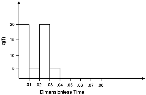
Some of the traditional forms of regularization and smoothing in inverse heat conduction problems, such as Tikhonov regularization and the function specification method are explained in classical texts such as Beck et al.[1] These traditional techniques facilitate smoothing of the calculated heat flux values, avoiding the extreme instabilities inevitable in non-regularized solutions, or what might be called ‘exact matching’. In contrast to these tools, the present research involves a type of heating which is presumed to have occurred over a relatively short amount of time in comparison with the time duration of the measured data. The experiment examined here as an example problem takes place over a dimensionless time period of 0.5 and the heating takes place over only 0.04 units of dimensionless time. More detailed information specifically on Tikhonov regularization can be found in Tikhonov and Arsenin [2]. One drawback to this type of regularization is the addition of bias to the solution. Since the regularization factor is added to the matrix equation during the solution process, a bias can be introduced which will tend to raise or lower all of the calculated heat flux values. Another drawback is that prior information can be required in order to use this type of regularization. A method similar to this is presented by Beck and Arnold [3] except that no prior information is required. The regularizing parameter is a scalar chosen by the user and the method typically involves minimizing the difference between the parameters being estimated and some other chosen quantities. Once again, this method necessarily introduces bias into the problem, with a larger regularization parameter introducing a larger amount of bias.

The present research, by contrast, utilizing the method of derivative regularization, employs the principle of matrix pre-multiplication to reduce the ill-conditioned nature of the matrix structure.[4] The use of a pre-conditioning method is fairly straightforward; however, the difficult and most critical aspect of this method lies in the development of the pre-conditioning matrices for the specific type of problem. Typically, the preconditioning matrix is constructed by working backward, in somewhat of a trial-and-error process, to develop a pre-conditioning matrix, which improves the structure of the problem without adding an unacceptable amount of error.

As the name implies, derivative regularization employs the time derivatives of the sensitivity coefficients and of the measured data in developing a pre-conditioning matrix to reduce the ill-posed nature of the inverse heat conduction problem. While the additive forms of regularization generally introduce bias, the derivative regularization method presented here carries the advantage of being unbiased. However, this unbiased advantage can sometimes come at the cost of larger estimation errors. An application of derivative regularization is given in [5], for a non-linear parameter estimation problem. The present research applies the derivative regularization method to the inverse heat conduction problem. Since the inverse heat conduction problem is linear, as opposed to the nonlinear problem studied in [5], an investigation can be made into the error induced by varying the weighting factors applied to the first and second derivative contributions to the regularization method. Indeed, convergence was not obtainable with many of the non-linear cases studied in [5]. For this reason, the linear inverse heat conduction problem is used for studying a full range of weighting factors and the results from each combination of these factors.

Attempts have also been made to measure heat-up rate in an experiment in addition to temperature. Frankel et al. [6] use temperature rate measuring sensors to improve robustness in heat transfer problems. As with other methods of regularization, the emphasis of the work described there is on smoothing of the calculated heat fluxes. Similarly, Frankel et al. [7,8] have used rate sensors in a number of other inverse heat conduction problems to enhance the stability of the analysis. In the present research, the heat-up rate is calculated by the use of parabolic splines which are fitted to the measured temperature data. From these splines, the instantaneous heat-up rate can be calculated using only temperature data so that a rate sensor is not required. This allows the effect of the temperature sensor on the experiment to be minimized, since only a thermocouple is needed, and the method can be used with non-contact optical temperature measurement systems as well. Moreover, the second derivative of the temperature data as a function of time is also calculated with this method which is shown to be a very important factor affecting the robustness of the heat flux calculation.

As noted earlier, the derivative regularization method is quite different from other methods of regularization where the objective is smoothing or stabilization of the estimated heat flux estimates as a function of time. Rather, the objective of derivative regularization is to sharpen the accuracy of heat flux estimates which are known to have taken place over a short period of time. The method is intended for use in cases where there is a short-duration of heating and detailed information is needed about that brief period. This information is obtained by the application of matrix preconditioning to temperature measurements taken over a much longer period of time than the period of the heating.

2 Description of the method

The inverse heat conduction problem is typically addressed by using dimensionless temperature values for computing temperature solution values for various locations in a solid material at various times. This solution is generated by solving the transient heat conduction equation, expressed in dimensionless form as(1) $\frac{\partial T}{\partial t}=\frac{{\partial }^{2}T}{\partial x^2}\text{,}x\in [0\text{,}1]\text{,}t⩾0$(1)

The dimensionless boundary conditions in the case of the sample problem examined as part of this research are(2a) $-{\left.\frac{\partial T}{\partial x}\right|}_{x=0}=q(t)\text{and}{\left.\frac{\partial T}{\partial x}\right|}_{x=1}=0\text{,}t⩾0$(2a)

The initial condition for this problem is zero temperature throughout the material.(2b) $T(x\text{,}0)=0\text{,}x\in [0\text{,}1]$(2b)

The dimensionless terms in these equations are defined as(3) $T=\frac{T_{D}k}{q_{D}L}x=\frac{x_D}{L}t=\frac{\alpha t_D}{L^2}q=\frac{q_D{t}_D}{\rho {\mathit{cLT}}_D}$(3)

where T, x and t are dimensionless temperature, distance and time, respectively. The respective dimensional counterparts of these terms are T_D (K), x_D (m) and t_D (sec). Additionally, k is thermal conductivity (W/m²), c is specific heat (J/kg-K), L is the thickness of the material (m), ρ is density (kg/m³) and α is thermal diffusivity (m²/sec). As given in [1], if this problem is considered in a discretized form, a solution can be generated for the temperature on the non-heated side in response to a unit heat flux. The temperature rise on the non-heated side (x = 1) where the temperature measurements are presumed to be taken as a function of time in response to a unit heat flux taking place over the first measured time step is designated ${\varphi }_1(t)$. The same response to a unit heat flux taking place during the second time step would, likewise, be designated as ${\varphi }_2(t)$ and so on. If the magnitude of the heat flux at each of the time steps is designated q₁, q₂, q₃, etc., then by the principle of superposition, the temperature at the non-heated surface can be written as(4) $T(t)=q_1{\varphi }_1(t)+q_2{\varphi }_2(t)+\cdots +q_m{\varphi }_m(t)$(4)

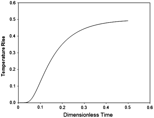
where the index m designates the number of time steps over which heat is applied. A plot of the heat fluxes used in testing this method is shown in Figure 1. Likewise, a plot of the temperature as a function of time in response to these pulses can be seen in Figure 2. As can be seen in this plot, the dimensionless temperature response settles at a temperature of 0.5 above ambient by the addition of the 0.5 dimensionless units of energy depicted in Figure 1.

Figure 1 The heat addition used in the derivative regularization test.

Figure 2 The temperature response from the four heat pulses used in testing the derivative regularization method.

Considering the full range of time steps during the course of the experiment, there are as many temperature values as there are time steps. These time steps are given the index n.

Therefore, the temperature solution can be expressed in matrix form as(5) $\mathbf{T}=X\mathbf{q}$(5)

where q represents the vector of unknown heat pulse magnitudes (m × 1), for each time step over which a non-zero heat flux exists on the heated side of the material. The X matrix (n × m) represents the dimensionless temperature response functions ${\varphi }_i(t)$ for the problem. Each row of the X matrix contains m dimensionless temperature rise terms, one for each of the heat flux values contained in the q vector. Through the principle of superposition, the product of X and q should be equal to the T vector (n × 1), which represents the temperature rise in response to the series of heat pulses. Since the q vector contains the unknown values in this over-defined set of equations, these values are found using least squares by pre-multiplying both sides of the equation by the transpose of the X matrix.[1] If the method of ‘exact matching’ was to be used, the final matrix equation to be solved for q would be(6) $X^{T}X\mathbf{q}=X^T\mathbf{T}$(6)

At this point, in an attempt to reduce the extent to which this problem is ill-conditioned, various methods have been used which impart structure to the square sensitivity matrix (X^TX) by adding a regularization term, such as with Tikhonov regularization.[2] In the case of derivative regularization, the derivatives of the temperature measurement curve are found by using parabolic splines fitted to the measured temperature data as well as to the calculated unit heat flux functions. One purpose of the splines is to provide a smoothing effect so that the effects of noise can be reduced by incorporating neighbouring points. Of course conventional filtering techniques can also be used for smoothing laboratory data; however, filtering was not used in the present case since errors are being superimposed on synthetic data. An odd number of points is always used for the splines so that the centre point of the spline can be used for information related to the point of interest on the curve. The number of points in each spline is selected somewhat subjectively based on the frequency of the noise. One spline is found for each of the points in the temperature history except for the points at the very beginning and end of the data file where an insufficient number of data points is available to form a full-length spline. The first derivative of the spline is evaluated at the centre of the spline and, since the spline is second-order, the second derivative is constant throughout the spline.

A new ‘sensitivity matrix’ is defined as follows(7) $\tilde{X}=\left[\begin{array}{c}\hfill X\hfill \\ \hfill w_1{X}^{\prime }\hfill \\ \hfill w_2{X}^{\prime \prime }\hfill \\ \hfill \hfill \end{array}\right]$(7)

where $X\prime$ represents a matrix made up of the same elements as the X matrix, but with each element consisting of the time derivative of the X matrix. Likewise, $X\prime \prime$ represents a matrix made up of the same elements as the X matrix, but with each element consisting of the second time derivative of the X matrix. The terms w₁ and w₂ are scalar weighting factors to control the amount of contribution of the first and second derivatives in the overall matrix composition. Therefore, the $\tilde{X}$ matrix carries dimensions of 3n × m since it has the same number of columns as the X matrix but has three times as many rows. This is because, for each time step, the $\tilde{X}$ matrix has three rows: one being the same as the applicable row in the X matrix, in addition to a row for the first derivative and a row for the second derivative for that time step.

Similarly, there is a $\tilde{T}$ matrix which is composed in the same way as the $\tilde{X}$ matrix. Specifically(8) $\tilde{\mathbf{T}}=\left[\begin{array}{c}\hfill \mathbf{T}\hfill \\ \hfill w_1\mathbf{T}\prime \hfill \\ \hfill w_2\mathbf{T}\prime \prime \hfill \\ \hfill \hfill \end{array}\right]$(8)

The $\tilde{\mathbf{T}}$ matrix, of course, has dimensions of 3n × 1 for the same reason as noted above for the $\tilde{X}$ matrix. With these modified matrices, the equation for the unknown heat fluxes now becomes(9) $\tilde{X}\mathbf{q}=\tilde{\mathbf{T}}$(9) And using least squares, pre-multiplying both sides by ${\tilde{X}}^T$, the equation becomes(10) ${\tilde{X}}^T\tilde{X}\mathbf{q}={\tilde{X}}^T\tilde{T}$(10)

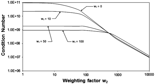
One way of quantifying the degree to which an inverse problem is ill-posed is by evaluating the condition number of the matrix used in the final calculation of the unknown heat pulse magnitudes. The gain in ability to compute parameters resulting from the use of this method was shown in quantitative form in [5] by comparing the condition number of the square ${\tilde{X}}^T\tilde{X}$ matrix, using the method given in Ref. [9]. If the weighting factors were to be assigned a value of zero, of course, Equation (10) would be equivalent to Equation (6). 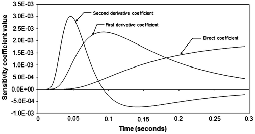Figure 3 shows a graph of the condition number of the ${\tilde{X}}^T\tilde{X}$ matrix as a function of the weighting factors, w₁ and w₂. As can be seen in this figure, an increase in the weighting factors leads to a reduction in the condition number. Moreover, as w₂ becomes large, the value of w₁ has very little effect. Insight can be obtained into the effect of introducing derivative information into the problem by examining the sensitivity coefficients. Figure 4 shows a plot of the sensitivity coefficients for the zeroth, first and second derivatives of the transient data. A reduction in the ill-posed nature of the problem is brought about by having uncorrelated sensitivity coefficients. Indeed, the second derivative has a larger magnitude in this case than the other curves, underscoring the effect of exploiting the rapid change in the shape of the temperature response curve at a certain critical time following the impartation of the heat pulse. The information measured at this critical time is magnified by the application of the weighting factors to the derivative information, making the calculation of the unknown heat flux values more robust. It is interesting to note that the largest effect of each of the curves in Figure 4 occurs at an earlier time as the derivative values become higher. Matching each of these corresponding derivative curves for the measured and calculated temperature curve is part of what gives the derivative regularization method its extra measure of robustness.

Figure 3 The condition numbers as functions of weighting factors for the ${\tilde{X}}^T\tilde{X}$ matrix.

Figure 4 The temperature response curve to pulse heating, along with the first and second derivatives.

If errorless temperature measurements are used, there is no need for derivative regularization, and the heat fluxes can be calculated using the exact matching method. The results in this case are accurate to approximately seven significant digits. However, as measurement errors are introduced, exact matching is no longer a viable method. Figure 5 shows the total of the absolute values of the errors between the actual and the estimated heat pulse magnitudes used in a number of test cases. The total error was found by adding the absolute values of the errors computed by the inverse method when compared to the four known heat flux values. In equation form, the total error can be expressed as(11) ${\epsilon }_{\text{q}}=|{\text{q}}_{\text{1est}}-{\text{q}}_1|+|{\text{q}}_{\text{2est}}-{\text{q}}_2|+|{\text{q}}_{\text{3est}}-{\text{q}}_3|+|{\text{q}}_{\text{4est}}-{\text{q}}_4|$(11)

Figure 5 The total error in estimated heat flux obtained using derivative regularization with an imposed measurement error standard deviation of 0.0001 dimensionless temperature units.

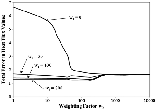
where ϵ_q is the total absolute value of the errors between the estimated and the known heat flux values, q_1est, is the estimated value of the first heat pulse and q₁ is the true magnitude of the first heat pulse. The standard deviation of the applied Gaussian temperature error in Figure 5 is 0.0001 dimensionless temperature units. The error was generated using the expression in Equation (12) which is found in [1].(12) ${\epsilon }_T=C\sqrt{\log (A)}\cos (2\pi B)$(12)

In this equation, ϵ_T is the imposed error on the dimensionless temperatures, A and B are uniformly distributed random errors and C is a constant affecting the standard deviation of the errors.

As can be seen in Figure 5, the heat flux error is rapidly reduced with the addition of either first or second derivative information (i.e. when either w₁ or w₂ are increased above zero). The non-regularized case (i.e. w₁ = 0 and w₂ = 0) gives an error of approximately 6.65 against a true value of 50 for heat flux. Once an adequate amount of regularization is added, this error drops to 1.31 dimensionless units. Similar to Figure 5, Figures67 show plots of the total error in heat flux for other values of measurement error. In both these cases, the results are found to be similar to those depicted in Figure 5. In general, as the weighting factors are increased, the estimation error is reduced until it reaches a minimum limit. Beyond this point, increasing the weighting factors does not bring about any additional reduction in estimation error. This seems to happen at values of w₂ = 1000, regardless of the value of w₁, the first derivative weighting factor. Table 1 summarizes the total estimation error in the regularized and non-regularized cases for each of the three figures, each of which is exposed to a different standard deviation of measurement error. In each of the three different cases of measurement error, the total estimation error is reduced by roughly a factor of three. Naturally, as the measurement error increases, the estimation error increases as well, for both the regularized and non-regularized cases. However, derivative regularization is found to reduce the estimation error in each case. Moreover, using large weighting factors gives essentially the best results in each case. What this seems to suggest is that, if the derivative information is weighted much heavier than the measured data, and the results are as good, or better, than with light weighting on the derivative information, then the derivative information is actually more useful than the direct measured temperature information. In other words, there seems to be no loss in the accuracy in the results if the direct temperature data (the zeroth derivative) are discarded. This seems to be consistent when comparing the sensitivity coefficients in Figure 4. The direct temperature history provides little other than a measure of the total amount of energy deposited in the material by the heating.

Figure 6 The total error in estimated heat flux obtained using derivative regularization with an imposed measurement error standard deviation of 0.0005 dimensionless temperature units.

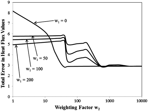
Figure 7 The total error in estimated heat flux obtained using derivative regularization with an imposed measurement error standard deviation of 0.001 dimensionless temperature units.

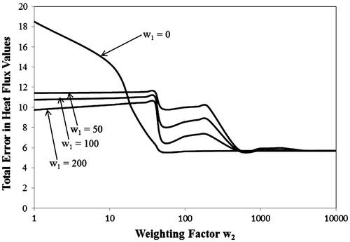
Table 1. Estimation error for non-regularized and regularized cases.

Standard deviation of measurement errors (dimensionless temperature)	Estimation error for non-regularized cases (dimensionless heat flux)	Estimation error for regularized cases (dimensionless heat flux)
0.0001	6.65	1.31
0.0005	8.17	2.91
0.001	18.5	5.68

3 Conclusions

A method of matrix pre-multiplication was developed using derivatives of measured and calculated temperature curves. This method was found to reduce the condition number of the matrix equations used, facilitating greater accuracy in the calculation of the unknown heat flux values through providing structure to the equations. This structure comes about through the uncorrelated nature of the temperature response curve and its derivatives. Weighting factors must be selected for the first and second derivatives used in the method. The method was demonstrated on a series of test cases which reduced the error in the calculated heat flux values by a factor of approximately three when compared to the non-regularized cases. The same benefits could be derived from any type of inverse problem where detailed information is desired about a short-term incident that generates a longer term response.

Table

Nomenclature
A, B	uniformly distributed random errors
C	coefficient affecting the standard deviation of temperature errors
c	specific heat (J/kg-K)
k	thermal conductivity (W/m-K)
L	material thickness (m)
m	heat flux index
n	temperature measurement index
qD	dimensional heat flux (W/m^2)
q	dimensionless Heat Flux
q	heat flux vector
t	dimensionless time
tD	dimensional time (s)
T	dimensionless temperature
TD	dimensional temperature (K)
T	temperature measurement vector
$\tilde{\mathbf{T}}$	transformed temperature measurement vector
xD	spatial dimension (m)
x	dimensionless distance
X	sensitivity matrix
$\tilde{X}$	transformed sensitivity matrix
w1	weighting factor for the first derivative of temperature
w2	weighting factor for the second derivative of temperature
$\alpha$	thermal diffusivity (m^2/sec)
${\epsilon }_q$	total error in dimensionless heat pulse estimation
${\epsilon }_T$	error applied to synthetic dimensionless temperature measurements
${\varphi }_m(t)$	temperature response as a function of time for unit heat pulse m
$\rho$	density (kg/m^3)

References

- Beck J, Blackwell B, St. Clair CR. Inverse heat conduction. New York: J. Wiley; 1985.
- Tikhonov A, Arsenin V. Solutions of ill-posed problems. Washington, DC: VH. Winston and Sons; 1977.
- Beck J, Arnold K. Parameter estimation. New York: J. Wiley; 1977.
- Golub G. Matrix computations. Baltimore, MD: Johns Hopkins University Press; 1989.
- McMasters R, Beck J. Using derivative regularization in parameter estimation. Inverse Prob. Eng. 2000;8:365–390.
- Frankel JI. Regularization of inverse heat conduction by combination of rate sensors analysis and analytic continuation. J. Eng. Math. 2007;57:181–198.
- Frankel JI. Generalizing the method of kulish to one-dimensional unsteady heat conducting slabs. AIAA J. Thermophys. Heat Transfer. 2006;20:945–950.
- Frankel JI, Osborne GE, Taira K. Stabilization of ill-posed problems through thermal rate sensors. AIAA J. Thermophys. Heat Transfer. 2006;20:238–246.
- Conte S, de Boor C. Elementary numerical analysis. New York: McGraw-Hill; 1980.