Synthesis of compact wind profiles using evolutionary algorithms

Abstract

In this paper, the authors face the problem of wind speed processing as environmental variable of a wind turbine system. Generally, the information on wind speed measurements is processed over long periods of time to be relevant with respect to the site characteristics (average and maximum speeds, statistics). Subsequent large scale profiles of wind speed lead to long processing time for simulation analysis and especially for optimization design that penalises the search of optimal solutions. An original synthesis approach of a compact and representative wind speed profile using an Evolutionary Algorithm (EA) is proposed. This approach is compared to a purely statistical approach based on random number generators. It allows reducing the actual wind profile duration with compression ratios greater (two months of wind speed measurements are compressed in only 1 h). Then, the synthesis approach by EA is applied to the sizing of an autonomous hybrid system based on wind turbine with battery storage for stand-alone energy systems. It has proven its effectiveness in reducing 200 days of wind speed measurements in only 10 days, allowing sizing the storage system with a significant gain in terms of computing time in the framework of the optimization process.

Keywords:

• wind profile synthesis
• evolutionary algorithm
• inverse problem
• statistical analysis
• wind turbine system

1. Introduction

This study is part of a system design approach for a wind turbine for which the sizing environmental variable is the wind speed. Because of its intermittent and fluctuating features, it is mandatory to assess the statistical characteristics of this primary energy vector. For that purpose, various methods have been then developed in order to provide temporal wind profiles.[1–5] Nevertheless, those approaches generally require the simulation of wind over long periods of time in order to evaluate the efficiency of a given system. This can be an important drawback in a context of integrated design by optimization [6] where the system simulations have to be repeated according to design variable variations. This issue was particularly shown in [7,8] through the example of a passive wind turbine sized from an optimization approach. In such case, the computing time required for sizing optimal wind turbine solutions strongly depends on the wind speed profile duration used to characterise the system behaviour and its efficiency. Therefore, it is thus advisable to consider a wind speed profile of minimum duration but which remains relevant with regard to the objectives and constraints in the integrated design process.

In [9], the authors propose to solve this problem by generating a wind speed profile with a reduced duration based on the use of classification methods. Their approach consists in merging into one class, temporal sequences characterised by similar statistical distributions. The similarity between the distributions of temporal sequences to be classified can be described by the first statistical moment (average, standard deviation) or more precisely by the overall characteristics of the statistical distribution by considering all statistical moments.[10] The representative temporal profile of each class is a real sequence of 10 min duration. Three classes of typical wind were identified from 10⁶ temporal wind speed sequences of 10 min measured at the site of ‘Petit Canal’ in Guadeloupe.[10]

In this paper, two synthesis approaches of wind speed profile with reduced duration are studied. The first concerns a purely statistical approach established in [11] and is based on random number generators for which the associated probability density functions are derived from the statistical distribution of real wind speed measurements. Complementary to this study, the authors propose a more realistic consideration of the fast wind speed dynamics characteristic of the turbulence phenomenon. The second approach is based on a synthesis process of a representative and compact wind speed profile. It consists of generating a fictitious compact profile for which the characterization indicators (maximum and average speeds, wind energy content) correspond to the real data reference characteristics. This compact and simplified profile is obtained by solving an inverse problem by aggregating elementary segments whose parameters are determined using an Evolutionary Algorithm (EA). The suggested EA-based approach can be viewed as a ‘compaction’ method but is radically different from traditional compression techniques used in signal and image processing described in [12]. It only preserves some signal features represented by typical targets or indicators that can be useful in a particular context (e.g. wind speed features which are relevant with regard to the sizing of electrical components of wind turbines).

Finally a comparative study of both approaches for the same simulation cost is established and the synthesis process of wind speed representative profile is applied for sizing an autonomous hybrid system based on wind turbine and batteries as storage elements.

2 Statistical based synthesis approach

The first synthesis method of a wind speed profile is based on a purely statistical approach. It consists in generating a continuous temporal profile from the statistical distribution of the measured wind speed. Among the probability rules (density) that can characterise the statistical distribution of the average wind speed, we note the log-normal distribution, the Gaussian distribution and the Weibull distribution.[13–15] This latter distribution is often more appropriate to describe statistical properties of the average wind speed.[16,17] The expression of the probability density of the Weibull distribution according to the average wind speed ($\overline{v}$) is:(1) $f(\overline{v})=\frac{k}{c}{\left(\frac{\overline{v}}{c}\right)}^{k-1}\exp \left(-{\left(\frac{\overline{v}}{c}\right)}^k\right)$(1) where k is the shape factor and c is the scale parameter related to the average wind speed.

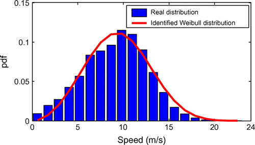
The Figure 1 shows the wind speed distribution for two months of measurements on the site of ‘Petit Canal’ in Guadeloupe with a sampling step of 10 min. This distribution is identified as a Weibull distribution (k = 3.03 and c = 10.62) from a standard least mean square algorithm.

Figure 1 Identification of the wind speed statistical distribution on the site of ‘Petit Canal’ at a Weibull distribution.

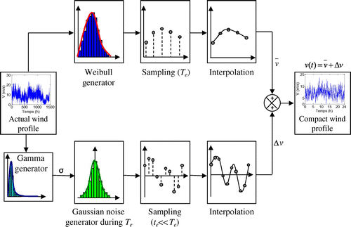
In a previous study,[11] the instantaneous wind speed has been decomposed in two different dynamics: a slow dynamic, which characterises the variation of the average wind speed according to a Weibull distribution and a fast dynamic characterising the turbulence phenomenon according to a Gaussian distribution [18] (see Figure 2). Note that the wind turbulence is an important phenomenon because it is coupled to mechanical stress of wind turbines.

Figure 2 Generating process of the wind speed representative profile based on statistical approach.

According to the slow dynamic, the statistical approach consists in generating a wind speed signal satisfying a statistical distribution established from data of the average wind speed measured in intervals of 10 min.[19] A certain number of samples is generated with a random number generator according to the established statistical distribution.

In the case of a Weibull distribution, the random number generator W(c, k) is defined from the inverse transformation of the cumulative distribution function associated with the probability density given by Equation (1). Referring to a random number generator with uniform density in the interval [0, 1] (U(0, 1)) and knowing the parameters of the Weibull distribution (c and k), the expression of the random number generator W (c, k) is given by Equation (2).[20](2) $W(c\text{,}k)=c{\left(-\ln U(0\text{,}1)\right)}^{\frac{1}{k}}$(2) The continuous temporal profile is then obtained by the interpolation of the N_e generated samples. The integration of the wind turbulence in the temporal profile is performed according to the fast dynamic. On each sampling period T_e of the slow dynamics, wind turbulence is modelled by a Gaussian noise with a mean equals to zero (μ = 0) and a standard deviation σ. The representative signal of the turbulence is generated from a random number generator with Gaussian density. The same principle as the Weibull density generator is used (see Figure 3) except that the sampling period t_e is very small compared to T_e. Finally, the wind speed representative profile is obtained by the sum of the slow component ($\overline{v}$) generated from the Weibull density and the fast component ($\mathrm{\Delta }v$).

Figure 3 Wind speed statistical distribution on the site of ‘Petit Canal’ in Guadeloupe on some temporal windows of 10 min.

In [11], the standard deviation σ of the Gaussian distribution (i.e. the turbulence intensity) was considered as constant along the generated wind speed profile. In this paper, we propose to make the statistical approach more realistic by generating the turbulence (Gaussian noise) with a variable standard deviation σ. Through an analysis phase of measured wind speed data, the distribution of the fast component is identified, on each interval i of duration T_e, to a Gaussian distribution characterised by a standard deviation σ_i. Next, we determine the statistical distribution D_σ of the standard deviations (σ_i). In the generated wind speed profile, on each sampling period T_e, the standard deviation of the Gaussian noise is determined from a random number generator based on the same probability density as the statistical distribution of standard deviations (D_σ) (see Figure 2).

The Figure 3 shows the wind speed statistical distribution on the site of ‘Petit Canal’ in Guadeloupe on some temporal windows of 10 min. We verify that these distributions follow a Gaussian function with parameters (μ, σ), centred on the mean value of the slow component of the wind speed over the temporal window of 10 min:(3) $f(v)=\frac{1}{\sigma \sqrt{2\pi }}\exp \left(-\frac{(v-\mu {)}^2}{2{\sigma }^2}\right)$(3)

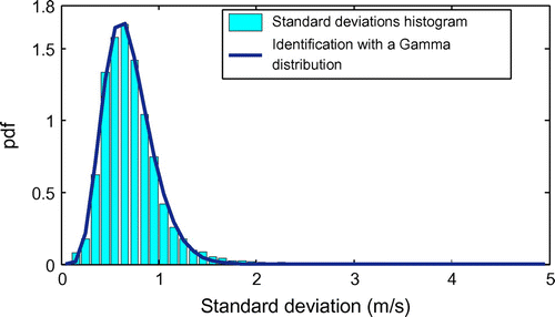
The statistical distribution D_σ of standard deviations (σ_i) on two months of wind speed measurements on the site of ‘Petit Canal’ is given by the histogram of Figure 4. This distribution is identified from a standard least mean square method with a Gamma density with α = 7.9 and β = 11.3 as parameters. 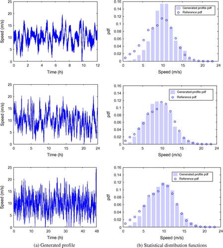The corresponding probability density f(σ) is given by Equation (4).[20](4) $f(\sigma )=\frac{{\beta }^{\alpha }}{\mathrm{\Gamma }(\alpha )}{\sigma }^{\alpha -1}\exp (-\beta \sigma )$(4) where Г is the Gamma function. The inversion of the cumulative distribution function associated with this probability density allows generating the turbulence intensity in the synthesis process of Figure 2. Three simulation results of the statistical approach for the generation of a wind speed profile (12, 24 and 48 h duration) are given in Figure 5(a): these synthesised profiles are representative of two months of wind speed measurements on the site of ‘Petit Canal’. The sampling period of the wind slow component T_e is set to 10 min and that of the fast dynamics (turbulence) t_e is fixed to 1 s. Those values are in accordance with the corresponding frequencies issued from the well-known Van der Hoven’s spectral distribution.[21,22] We then obtain respectively 72, 144 and 288 samples by the Weibull generator (k = 3.03 and c = 10.65) and 600 samples by the Gaussian generator for each time interval T_e. The Figure 5(b) shows a comparison between the statistical distribution functions (pdf) of the generated (12, 24 and 48 h duration) and original (2 months duration) profiles. The more duration increases (the number of sample increases), the more generated profile pdf is similar to the reference pdf. We conclude that the statistical approach requires long durations to better represent the actual profile.

Figure 4 Statistical distribution of standard deviations associated with the turbulence.

Figure 5 Results of the statistical approach for a three time horizon: 12, 24 and 48 h.

Through an analysis of the fast dynamic of the obtained profile, it is shown that the statistical distribution of some temporal windows of 10 min does not exactly follow a Gaussian distribution. This difference is due to the strong wind speed variations between two successive samples obtained from the Weibull generator and distant of a period T_e. This phenomenon modifies the statistical distribution of the fast component of wind speed (initially a Gaussian distribution). To rectify this problem, one solution is to increase the sampling time of the Weibull generator (for example 5T_e instead of T_e) in order to enhance the decoupling of slow and fast dynamics. However, this solution is limited in terms of representative profile duration. Indeed, the choice of a sampling period multiple of T_e increases the generated profile duration and therefore increases the computing time of design models, being especially critical in an optimization context.

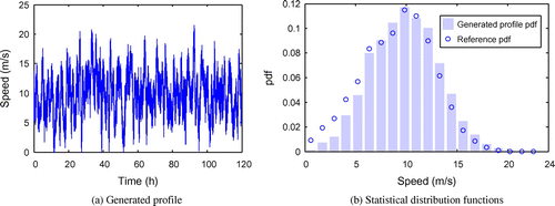
We present in Figure 6, a simulation of the statistical approach with a sampling period of 5T_e (the samples obtained by Weibull generator are separated by 5T_e = 50 min). We obtain a profile with a duration of 120 h (5 days) having a statistical distribution (pdf) very similar to the reference distribution that characterises the two months of wind speed measurements on the site of ‘Petit Canal’ (see Figure 6(b)). Furthermore, one can verify that the statistical distribution of the generated fast dynamics follows a Gaussian distribution on each temporal window of 10 min (see Figure 7).

Figure 6 Results of the statistical approach for a time horizon of 120 h.

Figure 7 Wind speed statistical distribution on some temporal windows of 10 min of the generated profile (120 h).

In conclusion, this statistical approach allows generating wind speed profiles which are relatively realistic as long as the duration of the synthesised profiles is sufficiently high. However, it does not guarantee to be relevant with regard to the air mass acceleration. In other words, no constraints are imposed on the wind speed variations between two successive samples of the random number generators.

3 Compact and representative synthesis approach by EA

In this section, a second approach is proposed for synthesising a compact and representative profile of an actual wind speed profile. This approach consists in generating a fictitious wind speed profile by fulfilling some constraints (typically minimum, maximum and average values, and probability distribution function). These constraints are expressed in terms of target indicators that can be evaluated from a set of actual profiles or from a single reference profile of large duration (for example some months/years of data).

3.1 Principle

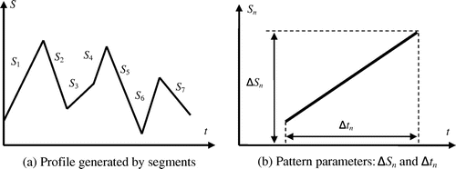
The synthesis process of compact wind profiles is based on the approach developed in [23] for railway driving missions. It consists in generating a fictitious profile of any environmental variable (e.g. temperature, wind speed, solar irradiation) by fulfilling some constraints related to the variables (typically minimum, maximum and average values and probability distribution function). These constraints are expressed in terms of target indicators that can be evaluated from a set of real cycles or from a single real cycle of large duration. The fictitious profile is obtained by aggregating elementary patterns (segments) as shown in Figure 8. Each segment is characterised by its amplitude ΔS_n (ΔS_min ref ⩽ ΔS_n ⩽ ΔS_max ref) and its duration Δt_n (0 ⩽ Δt_n ⩽ Δt_compact). A time scaling step is performed after the profile generation in order to fulfil the constraint related to the time duration, i.e. ΣΔt_n = Δt_compact. Finding a compact fictitious profile of an environmental variable consists in finding all segment parameters so that the generated profile fulfils all target indicators on the reduced duration Δt_compact. This results in solving an inverse problem with 2N_m parameters where N_m denotes the number of segments in the compact profile. This can be done using EAs [24,25] and especially with the clearing method [26] well suited to treat this kind of problem with high dimensionality and high multimodality.

Figure 8 Principle of the profile generation.

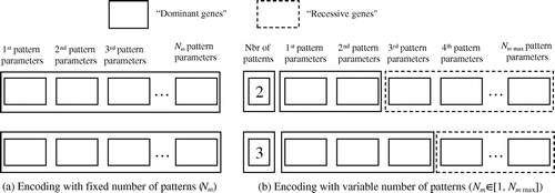
In addition to the choice of the parameters of each pattern, the EA is encoded so that the number of segments (N_m) can be itself optimised through a self-adaptive procedure.[23] Indeed, contrary to the classical chromosome encoding strategies which encods the same number of patterns for all individuals in the population (Figure 9(a)), a second strategy allowing the parallel investigation of signal configurations with distinct number of patterns is proposed (Figure 9(b)). It consists in encoding in the chromosome an additional gene representing the number of patterns. This number can vary from 1 to N_m max, N_m max denoting the maximum number of patterns. However, it should be noted that the chromosome is identical for all individuals in the population, containing the parameters associated with N_m max patterns. Then, only a part of the chromosome is considered in the individual decoding according to value of the gene associated with the number of patterns. The other genes are not expressed and can be considered as ‘recessive’. They are not used in the individual decoding but participate to crossover and mutation operations. Moreover, the EA is implemented using real-encoded decision variables, standard binary tournament selection, classical BLX-0.5 crossover [27] with maximum crossover rate (p_c = 1) and random mutation with probability p_m = 1/n where n denotes the total number of decision variables. The clearing procedure used as niching method is coded with a niche capacity of 1 and with a classical elitism scheme.[26]

Figure 9 Individual genotype according to the chromosome encoding strategy (with fixed or variable number of patterns).

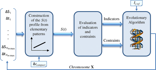
The synthesis process of wind speed profile by means of optimization is given in Figure 10. The aim is to minimize the error function ϵ expressed by Equation (5). This function represents the overall gap between the reference values of specific indicators (I_j ref) from the actual wind speed profile and those of the generated profile (I_j). These indicators will be detailed in the following subsection.(5) $\epsilon =\sum _j{\left(\frac{I_j(\mathbf{X})-I_{j\text{ref}}}{I_{j\text{ref}}}\right)}^2$(5)

Figure 10 Synthesis optimization process of wind speed representative profile.

In addition to the error function minimization, it may be necessary to impose some constraints on the generated profile (minimum and maximum values of standard deviation). These constraints (C_k) are formulated in terms of inequalities (C_k(X) ⩽ 0) and integrated into the error function in the form of penalties:(6) $\epsilon =\sum _j{\left(\frac{I_j(\mathbf{X})-I_{j\text{ref}}}{I_{j\text{ref}}}\right)}^2+\sum _k{\lambda }_k\max (0\text{,}{C}_k(\mathbf{X}){)}^2$(6)

where λ_k is a penalty factor associated to the kth constraint and X denotes an individual chromosome (real encoded vector containing the parameters of the elementary patterns).

3.2 Specific indicators of wind speed

An analysis phase of the wind speed in the temporal and statistical plan allowed us to propose a set of specific indicators related to the main design criteria of wind turbine systems:

• Maximum speed value: V_max

This indicator takes account of wind gusts when sizing the wind turbine.(7) $V_{\max }=\underset{t\in [0\mathrm{\Delta }{t}_{\text{profile}}]}{\max }V(t)$(7)

where Δt_profile denotes the duration of the reference wind profile.

• Average cubic wind speed value: ⟨V³⟩

The average cubic wind speed value ⟨V³⟩ is used instead of the average wind speed value ⟨V⟩ because the power produced by the wind turbine (P_WT) is directly proportional to the cubic wind speed value as shown in Equation (8).(8) $P_{\text{WT}}=\frac{1}{2}\rho C_{\text{p}}{\mathit{SV}}^3$(8)

where ρ denotes the air density in kg m⁻³, S indicates the area swept by the wind turbine blades in m², C_p represents the power coefficient defined by the ratio between the power captured by the wind turbine and the initial power of the air mass flowing through the area S at the speed V.

• Probability density function: pdf

It is relevant to take account of the wind speed statistical distribution (pdf) in the wind turbine design. The representative profile to be generated must then fulfil the same statistical distribution as the actual wind speed measured over a longer duration.

• The wind turbulence: I_turb

Wind turbulence is a crucial phenomenon in the estimation of the wind turbine lifetime (mechanical stress). It is then important to integrate an indicator to characterise the turbulence in the representative temporal profile. We then characterise the wind turbulence, on each interval i of duration T_e = 10 min, by the standard deviation σ_i.[28] We define the turbulence indicator I_turb of the wind profile by the average value of standard deviations σ_i.(9) $I_{\text{turb}}=〈{\sigma }_i〉\text{where}i=\left[1\text{,}\mathrm{integer}\mathrm{part}(\mathrm{\Delta }{t}_{\text{profile}}/T_{\text{e}})\right]$(9)

3.3 Results of the synthesis process of the representative profile

As previously, the reference values of the indicators are determined from two months of wind speed measurements on the site of ‘Petit Canal’ in Guadeloupe. Nevertheless, the choice of the representative profile duration is not obvious. Although the specific indicators of wind speed do not impose any minimum duration, the generated profile must include a sufficient number of samples in order to fulfil the reference statistical distribution (pdf_ref). The error function to be optimised is given by the following expression:(10) $\epsilon ={\left(\frac{V\max (\mathbf{\text{X}})-V\text{max ref}}{V\text{max ref}}\right)}^2+{\left(\frac{〈V{(\mathbf{\text{X}})}^3〉-{〈V^3〉}_{\text{ref}}}{{〈V^3〉}_{\text{ref}}}\right)}^2+{\left(\frac{I_{\text{turb}}(\mathbf{\text{X}})-I_{\text{turb ref}}}{I_{\text{turb ref}}}\right)}^2+{\epsilon }_{\text{stat}}$(10) where ϵ_stat represents the mean square error between the reference statistical distribution (pdf_ref) and that of the generated profile (pdf_gen) evaluated from 20 equal intervals of width V_{max ref}/20.(11) ${\epsilon }_{\text{stat}}=\frac{1}{20}\times \sum _{k=1}^{20}{\left(\frac{{\mathit{pdf}}_{\text{gen}}(\mathbf{X}\text{,}k)-{\mathit{pdf}}_{\text{ref}}(k)}{{\mathit{pdf}}_{\text{ref}}(k)}\right)}^2$(11)

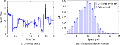
The Figure 11 gives a process result of a representative profile with a 3 h duration (compared with the initial duration of two months, i.e. almost 1500 h). The EA population size is set to 100 and the generation number is equal to 10⁵. The obtained number of elementary patterns (number of segments) is 217.

Figure 11 Synthesis process result of representative profile of a 3 h duration.

The characteristics of the generated wind speed profile are given in Table 1. The obtained results are perfect in the sense of specific indicators while two months of wind speed measurements (∼1500 h) are compacted in a ratio 500 (∼1500/3).

Table 1. Comparison of the generated profile indicators to the reference indicators.

	Reference indicators	Generated profile indicators	Error (%)
Vmax (m s^−1)	23.1	23.1	0.0
⟨V^3⟩ (m^3 s^−3)	1076	1076	0.0
Iturb	0.72	0.74	2.7

A second solution to enhance compacity of the generated profile duration is to integrate the phenomenon of turbulence as a constraint in the synthesis optimization process. Instead of imposing an average standard deviation as turbulence indicator, a range of variation of the standard deviation between a minimum and a maximum value respectively σ_min and σ_max has been considered. The turbulence indicator is no longer represented by an optimization criterion but instead by the two constraints σ_min and σ_max. For two months of wind speed measurements on the site of ‘Petit Canal’, the standard deviation of wind speed intervals (T_e = 10 min) varies between σ_min = 0.05 m s⁻¹ and σ_max = 4.9 m s⁻¹. An illustration of this solution for one hour generated profile duration is given in Figure 12(a). This wind speed profile is obtained by the concatenation of 105 segments. The generation number is equal to 15,000 which only corresponds to 5 hours of computation with a standard computer (Core Duo 2 GHz). Note that, despite the complexity of the inverse problem (211 parameters), the EA converges towards a very convenient solution respecting the constraint related to the turbulence phenomenon. Indeed, the Figure 12(b) shows that the statistical distribution of the generated profile perfectly corresponds with the reference distribution. The Table 2 also shows the low difference between the reference indicators and the generated profile indicators.

Figure 12 Synthesis process result of representative profile of a 1 h duration.

Table 2. Comparison of the generated profile indicators to the reference indicators.

	Reference indicators	Generated profile indicators	Error (%)
Vmax (m s^−1)	23.1	23.1	0.0
⟨V^3⟩ (m^3 s^−3)	1076	1078	0.2

Finally, the synthesis approach by EA is very efficient in terms of accuracy and reduction of the real wind speed profile duration. Indeed, two months of wind speed measurements are compressed in 1 h only. Consequently, this reduction provides a significant gain in terms of computing time which is particularly useful in the framework of wind turbine system design by optimization.

4 Comparison of the two synthesis approaches

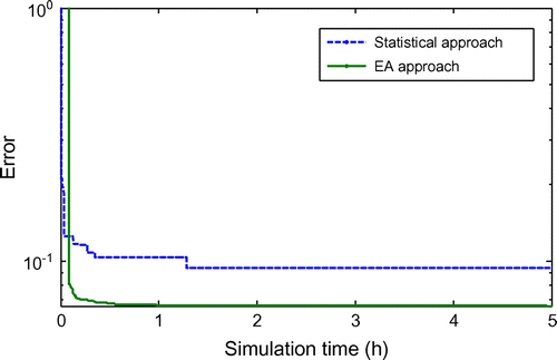
In this section, the statistical synthesis approach is compared with the EA-based synthesis approach by considering the same conditions in terms of computation time with the same computer. 5 h of computation time are chosen which corresponds to the convergence time required for synthesis approach by EA to generate a representative profile from two months of wind speed measurements on the site of ‘Petit Canal’ in Guadeloupe. Regarding the statistical synthesis approach, we proceed to generate a wind speed profile by successive iterations during 5 h of computation time. At each iteration, the obtained profile is retained if it improves the same error function ϵ used in the synthesis approach by EA (see Equation (12)). This error function aims at simultaneously optimising the maximum wind speed value, the average cubic wind speed value and the statistical distribution. In order to simplify this comparison, the turbulence indicator has not been considered here. The error function evolution over 5 h of computation is given in Figure 13.(12) $\epsilon ={\left(\frac{V\max -V\text{max ref}}{V\text{max ref}}\right)}^2+{\left(\frac{〈V^3〉-{〈V^3〉}_{\text{ref}}}{{〈V^3〉}_{\text{ref}}}\right)}^2+\frac{1}{20}\times {{\displaystyle \sum _{k=1}^{20}\left(\frac{pdf(k)-pd{f}_{\text{ref}}(k)}{pd{f}_{\text{ref}}(k)}\right)}}^2$(12)

Figure 13 Error function evolution for the two synthesis approaches.

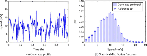
The representative profile duration is set to 1 h in the synthesis approach by EA and 5 days (120 h) in the statistical synthesis approach. This difference between the durations of representative profiles is related to the characteristics of each approach. Indeed, the statistical approach is not very relevant with short durations due to low number of samples while the synthesis approach by EA allows obtaining short duration profiles (1 h). The characteristics of the representative profiles obtained after 5 h of computing time on a standard PC (Core Duo 2 GHz) are given in Figure 14 and Table 3.

Figure 14 Comparison of generated profiles by the two synthesis approaches – time series and associated distributions.

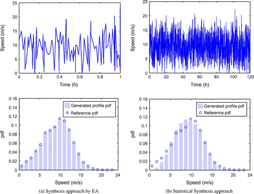
Table 3. Comparison of generated profiles characteristics by the two synthesis approaches.

	Vmax (m s^−1)	⟨V^3⟩ (m^3 s^−3)
Reference indicators	23.1	1076
Generated profile indicators
EA approach	23.1	1078
Statistical approach	22.2	1077
Error (%)
EA approach	0	0.2
Statistical approach	3.9	0.1

The obtained results show that the EA-based synthesis approach provides a better accuracy with respect to all indicators. In particular, the statistical distribution of the obtained profile perfectly follows the reference statistical distribution. Conversely significant differences can be observed in the case of the statistical approach (see Figure 14). In addition, the synthesis approach by EA leads to more compact duration of the representative profile. Indeed, two months of wind speed measurements are only represented by a profile of one hour duration.

5 Application of the synthesis approach by EA to a stand-alone wind system hybridised with storage

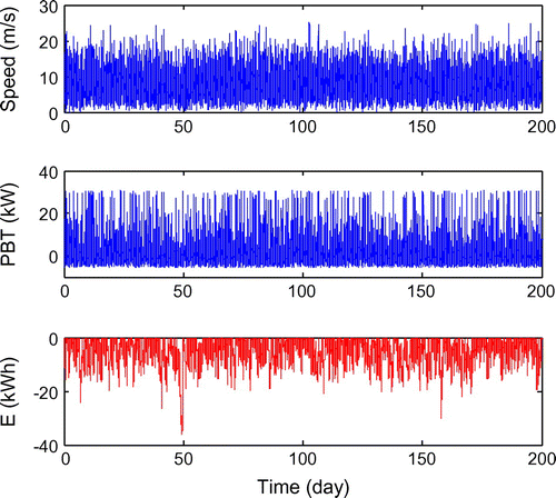
In this section, the interest of the compact and representative synthesis approach of a wind speed profile is illustrated on the sizing of a simple stand-alone system. The system is composed of a given 8 kW passive wind turbine [7,29] hybridised with a lead acid battery pack. The system is supposed to supply a periodic load profile P_load (24 h period). The problem here only consists in sizing the battery bank considering a given wind turbine and a wind farm potential represented by a reference wind profile resulting from 200 days of wind speed measurements. Unlike the previous case where the indicators are directly related to the wind speed characteristics, the indicators used in this application are also related to the sizing constraints on the storage system. Three particular indicators are considered: P_BTmax, P_BTmin and E_s which respectively denote the maximum and the minimum storage powers in the battery and the storage useful energy defined by Equation (13).[30] These indicators represent the physical variables required for the battery bank sizing.

The reference values of these indicators are extracted from the simulation of the wind speed actual profile of 200 days duration (see Figures1516). Note that the reference value of the storage useful energy E_sref is defined as follows:(13) $E_{\text{sref}}=\max E_{\text{BT}}(t)-\min E_{\text{BT}}(t)$(13) where $E_{\text{BT}}(t)={\int }_0^t{P}_{\text{BT}}(\tau )d\tau ={\int }_0^t(P_{\text{WT}}(\tau )-P_{\text{load}}(\tau ))d\tau t\in [0\text{,}200\text{days}]$

Figure 15 Extraction of indicator reference values from the actual wind speed profile of 200 days duration.

Figure 16 Actual reference wind speed profile and corresponding storage power/energy.

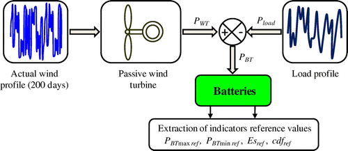
P_BT, P_WT and P_load are respectively the battery power, the power supplied by the wind turbine and the load power.

It should be noted that E_BT(t) is a saturated integral with 0 as upper limit so that the battery storage is only sized in discharge mode to avoid its oversizing during wide charge period (huge winds with reduced load). An additional target indicator is considered to take account of statistic features of the reference wind cycle. We use the cumulative distribution function cdf_ref computed from the corresponding probability density function pdf_ref related to the reference wind speed behaviour.[31] The pdf_ref is evaluated from 20 equally spaced intervals between 0 and the maximum wind speed value.

Finally, the global error ϵ to be minimised in the synthesis profile process can be expressed as:(14) $\epsilon ={\left(\frac{P_{\text{BT}\max }-P_{\text{BT}\max \text{ref}}}{P_{\text{BT}\max \text{ref}}}\right)}^2+{\left(\frac{P_{\text{BT}\min }-P_{\text{BT}\min \text{ref}}}{P_{\text{BT}\min \text{ref}}}\right)}^2+{\left(\frac{E_{\text{s}}-E_{\text{s}\text{ref}}}{E_{\text{sref}}}\right)}^2+{\epsilon }_{\text{stat}}$(14) where the statistic error ϵ_stat denotes the mean squared error between both cdfs relative to reference and generated wind speed profiles:(15) ${\epsilon }_{\text{stat}}=\frac{1}{20}\times \sum _{k=1}^{20}{\left(\frac{\mathit{cdf}(k)-{\mathit{cdf}}_{\text{ref}}(k)}{{\mathit{cdf}}_{\text{ref}}(k)}\right)}^2$(15)

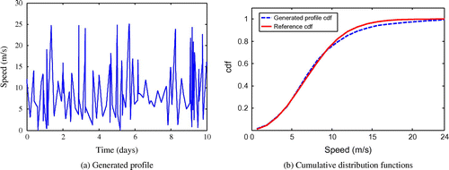
All ‘ref’ indexed variables are based on the reference wind profile of Figure 16. The inverse problem has been solved with the ‘clearing’ algorithm using a population size of 100 individuals and a number of generations of 500,000. Multiple optimization runs were performed with different compaction time Δt_compact. In particular, the minimum compaction time (i.e. min (Δt_compact)) was determined using dichotomous search in order to ensure a global error ϵ less than 10⁻². The Table 4 shows the values of the global error ϵ vs. the compaction time. It can be seen that the lowest value for Δt_compact ensuring the fulfilment of the target indicators with sufficient accuracy is about 10 days. The Figure 17 shows the characteristics of the generated wind profile obtained from the aggregation of 109 elementary segments fulfilling all target indicators. It can be seen from this figure that the cdf of this compact wind profile closely coincides with that of the reference wind profile.

Table 4. Influence of Δt_compact on the global error ϵ.

Δtcompact (days)	40	20	10	5
Global error ϵ	≈8 × 10^−3	≈9 × 10^−3	≈9 × 10^−3	≈7 × 10^−2

Figure 17 Synthesis process result of representative profile over a 10 days duration.

The Table 5 compares the values of the target indicators related to the battery sizing for the reference and the fictitious profile generated with the ‘clearing’ algorithm. A good agreement between those values indicates that the compact wind profile would lead to the same battery sizing as the reference wind profile with longer duration (200 days).

Table 5. Target indicators of the generated wind speed profile.

	Reference indicators	Generated profile indicators	Error (%)
PBTmax (kW)	30	30	0.0
PBTmin (kW)	−5.88	−5.82	0.1
Es (kWh)	32.36	32.4	0.12

6 Conclusion

In this paper, two different approaches have been developed for compacting wind speed profiles. The first concerns a purely statistical approach based on random number generators with probability density functions derived from the statistical distribution of actual wind speed data. The authors have proposed a more realistic consideration of the fast wind speed dynamics representative of the turbulence phenomenon.

In a second approach, a synthesis process of representative wind speed profile of reduced duration has been developed. This process is based on the aggregation or concatenation of elementary patterns which the number and the parameters are determined by an EA optimization. It allows synthesising a fictive and compact wind speed profile which verifies a set of pertinent indicators with regard to design criteria and constraints. Two months of wind speed measurements are compressed in only 1 h. Consequently, this reduction provides a significant gain in terms of computing time in the framework of the optimization process of wind turbines.

Then, a comparative study of the two synthesis approaches for the same computing cost has been established. Note that the synthesis approach by EA gives the advantage of a more compact duration of representative profiles.

Finally, the synthesis approach by EA was applied for sizing a stand-alone hybrid system based on wind turbine and batteries as storage elements. The indicators considered in this application are related to storage device features. The synthesis approach by EA has proven its effectiveness in reducing 200 days of wind speed measurements in only 10 days, allowing sizing the storage system with a significant gain in terms of computing time in the framework of the optimization process. Note that this synthesis approach is very generic, which can exceed the particular field of wind turbines design to be applied in the whole range electrical engineering applications and even beyond, by processing any types of environmental variables (wind speed but also temperature, sun irradiation, etc.) or for example of railway driving profiles as proposed in [23].

Acknowledgment

The authors would like to thank the GRER (Renewable Energy Research Group – Antilles Guyane) for availability of wind speed sequences measured at the site of ‘Petit Canal’ in Guadeloupe.

References

- Feijoo AE, Cidras J, Dornelas JLG. Wind speed simulation in wind farms for steady-state security assessment of electrical power systems. IEEE Trans. Energy Convers. 1999;14:1582–1588.
- Dobigeon N, Tourneret JY. Joint segmentation of wind speed and direction using a hierarchical model. Comput. Stat. Data Anal. 2007;51:5603–5621.
- Mohandes M, Rehman S, Halawani TO. A neural networks approach for wind speed prediction. Renewable Energy J. 1998;13:345–354.
- Damousis IG, Alexiadis MC, Theocharis JB, Dokopoulos PS. A fuzzy model for wind speed prediction and power generation in wind parks using spatial correlation. IEEE Trans. Energy Convers. 2004;19:352–361.
- Slootweg JG, de Haan SWH, Polinder H, Kling WL. General model for representing variable speed wind turbines in power system dynamics simulations. IEEE Trans. Power Syst. 2003;18:144–151.
- Roboam X, editor. Integrated design by optimization of electrical energy systems. London (UK): Wiley ISTE; 2012. Available from: http://www.eu.wiley.com/WileyCDA/WileyTitle/productCd-1848213891.html
- Tran DH, Sareni B, Roboam X. Integrated optimal design of a passive wind turbine system: an experimental validation. IEEE Trans. Sustainable Energy. 2010;1:48–56.
- Abdelli A, Sareni B, Roboam X. Model simplification and optimization of a passive wind turbine generator. Renewable Energy J. 2009;34:2640–2650.
- Calif R, Blonbou R, Deshaies B. Wind velocity measurements analysis for time scales smaller than 1 hour: application to wind energy forecasting. Proceedings of the 24th AIAA/ASME Wind Energy Symposium, Reno (NV); 2005.
- Calif R, Emilion R, Soubdhan T. Classification of wind speed distributions using a mixture of Dirichlet distributions. Renewable Energy. 2011;36:3091–3097.
- Roboam X, Abdelli A, Sareni B. Optimization of a passive small wind turbine based on mixed Weibull-turbulence statistics of wind. Québec: Electrimacs; 2008.
- Sayood K. Introduction to data compression. 4th ed. Waltham (MA): Morgan-Kaufmann; 2012.
- Joseph P, Hennessey J. Some aspects of wind power statistics. J. Appl. Meteorol. Climatol. 1977;16:119–128.
- Celik AN. A statistical analysis of wind power density based on the Weibull and Rayleigh models at southern region of Turkey. Renewable Energy. 2003;29:593–604.
- Weisser D. A wind energy analysis of Grenada: an estimation using the ‘Weibull’ density function. Renewable Energy. 2003;28:1803–1812.
- Keller JK. Simulation of wind with ‘K’ parameter. Wind Eng. 1992;16:307–312.
- Carta JA, Ramírez P, Velázquez S. A review of wind speed probability distributions used in wind energy analysis: case studies in the Canary Islands. Renew. Sustain. Energy Rev. 2009;13:933–955.
- Straroon DA, Stengelz RF. Stochastic prediction techniques for wind shear hazard assessment. J. Guid. Control Dyn. 1990;15:1224–1229.
- Nichita C, Luca D, Dakyo B, Ceanga E. Large band simulation of the wind speed for real time wind turbine simulators. IEEE Trans. Energy Convers. 2002;17:523–529.
- Law AM, Kelton WD. Simulation modeling and analysis. 2nd ed. New York: McGraw Hill; 1991.
- Van der Hoven I. Power spectrum of horizontal wind speed in the frequency range from 0.0007 to 900 cycles per hour. J. Atmos. Sci. 1957;14:160–164.
- Bianchi FD, Batista H, Mantz RJ. Wind turbine control systems: principle, modeling and gain scheduling design, advances in industrial control series. London: Springer-Verlag; 2010.
- Jaafar A, Sareni B, Roboam X. Signal synthesis by means of evolutionary algorithms. Inverse Prob. Sci. Eng. 2012;20:93–104.
- Schwefel HP. Evolution and optimum seeking. New York (NY): Wiley; 1995.
- Sareni B, Krähenbühl L. Fitness sharing and niching methods revisited. IEEE Trans. Evol. Comput. 1998;3:97–106.
- Petrowski A. A clearing procedure as a niching method for genetic algorithms. Proceedings of the IEEE International Conference on Evolutionary Computation; 1996; Nagoya, Japan.
- Eshelman LJ, Schaffer JD. Real-coded genetic algorithms and interval schemata. In Whitley D, editor. Foundations of genetic algorithms II; 1993. P. 187–202.
- Frandsen S, Thogersen M. Integrated fatigue loading for wind turbines in wind farms by combining ambient turbulence and wakes. J. Wind Eng. 1999;23:327–339.
- Belouda M, Belhadj J, Sareni B, Roboam X. Battery sizing for a stand-alone passive wind system using statistical techniques. 8th IEEE International Multi-conference on Systems, Signals and Devices (SSD); 2011; Hammamet, Tunisia.
- Belouda M, Belhadj J, Sareni B, Roboam X, Jaafar A. Synthesis of a compact wind profile using evolutionary algorithms for wind turbine system with storage. 16th IEEE Mediterranean Electrotechnical Conference; 2012; Medina, Yasmine Hammamet-Tunisia.
- Bagul AD, Salameh ZM, Borowy BS. Sizing of a stand-alone hybrid wind-photovoltaic system using a three-event probability density approximation. Sol. Energy. 1996;56:323–335.