
 ?Mathematical formulae have been encoded as MathML and are displayed in this HTML version using MathJax in order to improve their display. Uncheck the box to turn MathJax off. This feature requires Javascript. Click on a formula to zoom.
Abstract
This paper considers the boundary-value inverse heat conduction problem with steady boundary. To solve this problem, different approaches based on the Laplace and Fourier transforms are proposed. Application of the Laplace transform makes it possible to obtain an operator equation describing the explicit dependence of the desired boundary-value function on the initial data at the other boundary. This approach to solving the problem is used for the first time. The method based on the direct and inverse Fourier transforms with respect to the time variable provides stable solutions. The estimation of error of these solutions is the best with respect to the order. The range of application of each of the proposed methods and the stability of the solutions obtained by these methods was evaluated by a computational experiment.
Introduction
In experimental studies of non-stationary thermal processes, it is often impossible to directly measure the desired physical quantity, and its characteristics are therefore found from the results of indirect measurements. In this situation, one way to determine the desired physical quantity is to solve boundary-value inverse heat conduction problems. This paper presents methods for solving a fixed-boundary inverse heat conduction problem based on the Laplace and Fourier transforms.
The use of direct and inverse Laplace transforms to solve inverse heat conduction problems is of great interest. For example, Kolodziej et al. [Citation1] and Cialkowski and Grysa [Citation2] used the Laplace transform to solve the Cauchy problem. Monde et al. [Citation3] applied the Laplace transform to the two-dimensional problem.
In existing approaches, the equations resulting from the Laplace transform are usually solved by regularization methods, and the inverse transform is then applied to the regularized solution. However, the main difficulty in using the inverse Laplace transform is that this operation is highly unstable.
In this paper, a different approach is proposed. In this approach, the explicit dependence of the boundary function on one of the boundaries on the known data on the other boundary is described by an operator equation, and regularization methods are then used to solve this equation. This eliminates the need to perform the unstable procedure of numerical inversion of the Laplace transform in the computational process. The proposed method was used in a computational experiment to obtain a numerical solution of the inverse problem.
The Fourier transform with respect to the space variable has been widely used to solve the inverse heat conduction problems. In particular, Jonas and Louis [Citation4] applied the Fourier transform and a stabilizing functional to obtain regularized solutions. Prud’homme and Hguyen [Citation5] make use of the Fourier transform and a conjugate gradient for the purpose of regularization of solutions and evaluation of their convergence. Fu et al. [Citation6] and Qian and Feng [Citation7] took the direct Fourier transform with respect to the space variable and, as a result, obtained the Fourier transform of the solution of the inverse boundary-value problem.
The approach proposed in this paper is to use the direct and inverse Fourier transforms with respect to the time variable. The regularization algorithm is based on the projection regularization method for the direct and inverse Fourier transforms. This method provides regularized solutions with the best possible error bounds. This property provided the basis for comparative analysis of the solutions obtained by the Laplace and Fourier transform methods.
The developed methods were employed to perform a computational experiment. The objectives of this experiment were to test the performance of the algorithms and to evaluate the errors of the regularized solutions provided by each approach.
Statement of the problem
We consider the following inverse heat conduction problem:(1)
(1)
(2)
(2)
(3)
(3) In this problem, it is required to find the boundary value of the function:
(4)
(4) Let
for all
and there exists constants
such that
for all
for any
, where
is the Hölder space space and
.
It is known that for , there exists an exact solution
. However, instead of
we are given some approximations
and an error level
, such that
. Using these initial data, it is required to construct a regularized solution of the problem (Equation1
(1)
(1) )–(Equation4
(4)
(4) ).
Uniqueness of the solution of the problem (Equation1(1)
(1) )–(Equation4
(4)
(4) ) was proved in [Citation8]. In this paper, we propose methods based on Laplace and Fourier transforms to solve the problem (Equation1
(1)
(1) )–(Equation4
(4)
(4) ).
Construction of the operator equation using the Laplace transform
The problem (Equation1(1)
(1) )–(Equation4
(4)
(4) ) can be reduced to an integral equation. To do this, we find the solution of the direct problem, assuming that the required function
is known. Thus, we consider the following direct problem:
(5)
(5)
(6)
(6)
(7)
(7) It is required in this direct problem to find the function
for
.
Suppose that there exist such constants and
that for any
and for any
the following inequality holds
. In addition, we assume that the function
satisfies the Dirichlet conditions for
for any
. Then, we can apply the Laplace transform [Citation9] to function
for solving of the direct problem (Equation5
(5)
(5) )–(Equation7
(7)
(7) ). Such approach allows obtain an equation relating
and
.
Let be the Laplace transform of the function
, and
be the Laplace transform of the function
. Then, the operator representation of the problem (Equation5
(5)
(5) )–(Equation7
(7)
(7) ) is given by:
The solution of this problem has the following form:
(8)
(8)
Theorem 3.1
The function can be represented as:
(9)
(9)
Proof
Because the function has simple poles at the points
,
and the point
is a regular point of the function
and
it follows that the function
is meromorphic.
Consider a system of contours . Each contour contains only a finite number of poles and exists certain number
such that for any contour:
(10)
(10) Hence, we obtain the boundedness of the function for any contour.
Thus, for , we can use the Mittag–Leffler theorem on the expansion of functions in series of simple fractions, according to which the function
may be represented as the series:
(11)
(11) where
is the main part of the expansion of the function
at the poles
and
and
are given by the relations:
(12)
(12)
(13)
(13) Since the estimate (Equation10
(10)
(10) ) does not depend on
, the function (Equation11
(11)
(11) ) becomes:
(14)
(14) Cauchy’s theorem implies that
and, hence,
Substitution of the last relation into (Equation14
(14)
(14) ) yields:
Thus, the theorem is proved.
Applying the inverse Laplace transform to both the sides of (Equation8(8)
(8) ), using (Equation9
(9)
(9) ), the convolution theorem [Citation9] and the presence multiplier p in the second part in (), we obtain:
(15)
(15)
Theorem 3.2
Suppose that there exist such constant and
that for any
holds
. In addition, we assume that the function
satisfies the Dirichlet conditions for
for any
. Then, the series (Equation15
(15)
(15) ) converges all
and for
the solution
of the problem (Equation5
(5)
(5) )–(Equation7
(7)
(7) ) has the following form:
(16)
(16)
Proof
Because the function satisfies the Dirichlet conditions, using the properties of functionals in linear normed spaces [Citation11] and the estimate of the quantity
, for
we obtain:
The series
converges and the sum of this series is of the form
, where
is the Riemann zeta function and
, [Citation12]. Thus, the convergence of the series (Equation15
(15)
(15) ) follows from the Weierstrass theorem.
Using the property of convergent series and expanding the operator in the relation (Equation15
(15)
(15) ), we have that for
, the function
defined by the following relation:
(17)
(17)
The differentiation of the series (Equation17(17)
(17) ) with respect to the variable
presents some difficulties. However, since we only need the function
, we proceeded as follows. Following the ideas proposed in [Citation13] and [Citation14], we approximate the functions
as the truncated series:
(18)
(18) Since the function
is known, the solution of the problem (Equation1
(1)
(1) )–(Equation4
(4)
(4) ) reduces to solving the following equation:
(19)
(19) Using (Equation19
(19)
(19) ), it is required to find
(20)
(20) provided that, instead of
we know its approximations
and
such that for all
holds
.
Thus, the problem (Equation19(19)
(19) ),(Equation20
(20)
(20) ) is solved in two steps. The first step involves choosing an optimal number of terms in the partial sum of the series (Equation19
(19)
(19) ) and reducing the solution to solving an equation with a finite number of terms. Then, the resulting equation is solved using the method proposed by Lavrentiev.
To evaluate the effectiveness of the proposed approach, we performed a computational experiment and made a comparative analysis of the obtained solutions and solutions with the best possible error bounds. Solutions with the desired error bound were constructed using a method based on the Fourier transform with respect to the time variable and the projection regularization method.
Remark.
As one of anonymous referees has kindly pointed out to the author, the formula (5.9) of the paper [Citation15] is exactly formula () of Theorem 3.1. Still, the author believes that it makes sense to present the full proof of Theorem 3.1 here, because the above derivation of (Equation9(9)
(9) ) uses an idea which is different from the one in [Citation15].
Projection regularization method
Suppose that is a Hilbert space,
is a linear, injective, bounded operator,
, the spectrum
. We consider the operator equation:
(21)
(21) The lemma proved in [Citation16] implies the existence of a unitary operator
, such that the following polar decomposition of the operator
holds:
Let
be conjugate to
and
. The projection regularization method is proposed in and its regularization family
is defined by the formula:
(22)
(22) where
use the spectral decomposition of
generated by the operator
, and the regularization parameter
chosen as follows.
Let . Then, as the regularization parameter
we choose one of the solutions of the equation:
(23)
(23) Note that Equation (Equation23
(23)
(23) ) can have a several solutions. This fact does not affect the accuracy of the approximate solution of Equation (Equation21
(21)
(21) ).
The appearance of the number ‘9’ in (Equation23(23)
(23) ) is due to the proof of the optimality of the projection regularization method [Citation17]. The constant ‘9’ is an upper estimate of all possible occurring constants in this procedure. Although, one might probably obtain a lower constant, this one is sufficient for our goal.
In the proposed approach, the approximate solution of Equation (Equation21(21)
(21) ) is given by:
(24)
(24) where the operator
is given by formula (Equation22
(22)
(22) ), and
is one solution of Equation (Equation23
(23)
(23) ).
It has been proved previously [Citation17] that the operators given by the formula (Equation24(24)
(24) ) is a regularization method for Equation (Equation21
(21)
(21) )and the error estimate of the regularized solutions is the best with respect to the order. This property of regularized solutions provided the basis for comparative analysis of the numerical methods developed using Fourier and Laplace transforms.
Numerical simulation of the solution of the inverse problem for the Laplace transform
Let and
. The numerical scheme for solving the problem (Equation19
(19)
(19) ), (Equation20
(20)
(20) ) is as follows. The first step of the solution is to transform the initial data. For this, we orthogonalize the system of functions
for each
and denote the obtained orthogonalized system of functions by
. The function
is represented in terms of this system as:
(25)
(25) Then, the function
can be expressed as:
(26)
(26) Taking into account (Equation19
(19)
(19) ) and (Equation26
(26)
(26) ) and using the approach proposed in [Citation8], we find that the regularization parameter defined by formula (Equation23
(23)
(23) ) is the number of terms in the partial sum of the series (Equation26
(26)
(26) ). Thus, the regularization parameter is determined from the following equation:
(27)
(27) Let
be the number of terms found from (Equation27
(27)
(27) ). Then, Equation (Equation19
(19)
(19) ) is transformed to:
(28)
(28) If
for any
. Then, we use the following computational scheme for numerical solution of Equation (Equation28
(28)
(28) ). Let
(29)
(29)
then for any
at
Equation (Equation28
(28)
(28) ) becomes:
(30)
(30) It is necessary to find the function
from Equation (Equation30
(30)
(30) ). Thus, the solution of the problem (Equation1
(1)
(1) )–(Equation4
(4)
(4) ) reduces to solving a Volterra equation of the first kind, provided that
.
To solve the problem (Equation30(30)
(30) ), we use Lavrentiev method [Citation18]. According to this approach, the regularized solution of the problem is obtained from the equation:
(31)
(31) provided that
and the regularization parameter
may be chosen by various ways.
In our research the regularization parameter is chosen as follows. Let be a regularized solution of Equation (Equation31
(31)
(31) ). We set
and
. Following the idea proposed in [Citation19] and taking into account relation (Equation23
(23)
(23) ), we obtain that the regularization parameter is defined by the formula:
(32)
(32) The proposed method of solving the problem (Equation1
(1)
(1) )–(Equation4
(4)
(4) ) based on the Laplace transform was used to develop a numerical method consisting of the following steps.
Determining the number
of terms in the series (Equation28
Verifying the condition
Solving Equation (Equation31
Checking condition (Equation32
In order to test the reliability of the results and evaluate the effectiveness of the proposed scheme, we performed a computational experiment for a series of model examples. The experimental results were used for comparative analysis of the solutions obtained by applying the Laplace and Fourier transforms.
Numerical simulation of the inverse problem for the Fourier transform
We proceed to construct a numerical method based on the Fourier transform to solve (Equation1(1)
(1) )–(Equation4
(4)
(4) ). If it is known that the solution
of the direct problem (Equation5
(5)
(5) )–(Equation7
(7)
(7) ) satisfies the conditions:
and the function
such that
, then the Fourier transform with respect to the variable
can be used for solving of the problem (Equation1
(1)
(1) )–(Equation4
(4)
(4) ).
Let . We apply the Fourier transform
with respect to the variable
for
. Since the transform is used for
, it is necessary to perform the projection of the images onto
. Then, the function
corresponds to a function
such that:
(33)
(33) The regularization parameter
given by formula (Equation23
(23)
(23) ) is chosen to be the solution of the following equation:
(34)
(34) Applying the Fourier transform
with respect to the variable
, we find that the operator representation of the problem (Equation1
(1)
(1) )–(Equation4
(4)
(4) ) of the form:
(35)
(35)
where
,
.
Solving the problem (Equation35(35)
(35) ) and using the transformations (Equation33
(33)
(33) ), (Equation34
(34)
(34) ) we obtain the desired function
given by the formula:
(36)
(36) where
, the regularization parameter
satisfies Equation (Equation34
(34)
(34) ) and the function
is given by relation (Equation33
(33)
(33) ).
Applying the inverse Fourier transform to the function
, we get:
(37)
(37) Using the projection regularization method for the function
the regularized solution of the problem (Equation1
(1)
(1) )–(Equation4
(4)
(4) ) has the form:
(38)
(38) The proposed scheme (Equation33
(33)
(33) )–(Equation38
(38)
(38) ) was used to develop a numerical method for solving the problem (Equation1
(1)
(1) )–(Equation4
(4)
(4) ). The computational scheme of the method is as follows:
Apply the Fourier transform to the elements
Find the parameter
Transform the initial data according to formulas (Equation34
Find the Fourier transform
Obtain the regularized solution using formulas (Equation37
Computational results
To test the effectiveness of the proposed approaches and to perform comparative analysis of the solutions obtained, we performed a computational experiment for a series of model examples. In the experiment, the direct and inverse problems were solved and norms of the deviations of the regularized solutions from the model functions were determined. The model functions differed in the monotonicity and continuity of their derivatives. In each series, several recalculations for each function were perfumed.
The computational experiment was carried out for using a uniform grid of
points
, and
,
. The numerical experiments includes the following steps:
The direct problem (Equation5
The values of
The inverse problem (Equation1
The quantity
Fig. 1 Results of the numerical solution for the boundary function with
.
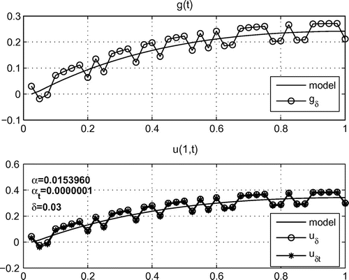
Example 1.
In this series of experiments, continuous monotonic functions were used. The experiment was performed for different levels of error. Figure shows the results of the numerical solution of the problem (Equation1(1)
(1) )–(Equation4
(4)
(4) ) for the model function
with
.
Example 2.
In this series of experiments, continuous smooth functions with a single extremum were used. The experiment was carried out for different levels of error. Figure shows the experimental results for one of the model functions with
.
Example 3.
In this series of experiments, continuous smooth function with several extremes were used. The experiment was carried out for different levels of error. Figure shows the results of numerical solution of the problem (Equation1(1)
(1) )–(Equation4
(4)
(4) ) for the function
with
, Figure shows the results of the experiment for the model function
with
.
Fig. 2 Results of the numerical solution for the boundary function with
.
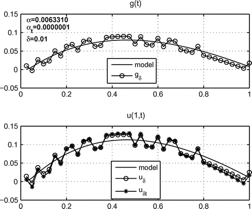
Fig. 3 Results of the numerical solution for the boundary function with
.
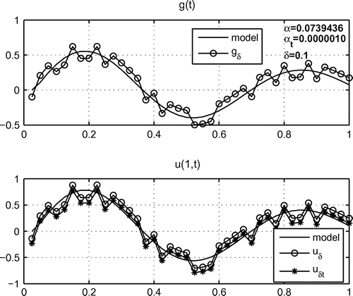
Fig. 4 Results of the numerical solution for the boundary function with
.
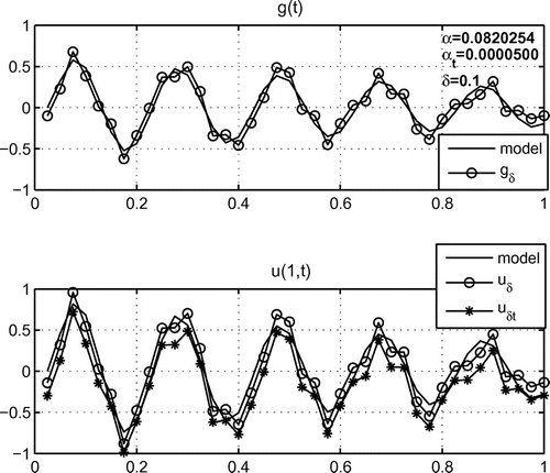
Fig. 5 Results of the numerical solution for the function .
![Fig. 5 Results of the numerical solution for the function u(1,t)={−40t,t∈[0;0.025],−1,t∈(0.025;0.5],80t−39,t∈(0.5;0.525],1,t∈(0.525;1]..](/cms/asset/12fd60d5-64f4-439f-8f04-4f912c035987/gipe_a_830614_f0005_b.gif)
Fig. 6 Results of the numerical solution for the function .
![Fig. 6 Results of the numerical solution for the function u(1,t)={sin(5πt)−2.5t2,t∈[0;0.5),cos(5πt),t∈[0.5;1]..](/cms/asset/372b82df-f803-4dbc-a0c5-64305e19996f/gipe_a_830614_f0006_b.gif)
Example 4.
In this series of experiments, continuous functions with discontinuous derivatives were used. A difficulty in this experiment was that Equation (Equation28(28)
(28) ) was reduced to the Volterra equation of the first kind, so that a necessary condition for the stability of the process was the continuity of the model function. The results of the numerical solution of the problem (Equation1
(1)
(1) )–(Equation4
(4)
(4) ) for
are presented in Figure , and in Figure .
To study the stability of the regularized solutions and obtain experimental estimates for the deviations of these solutions from the given model functions in each series of experiments, we measured the quantities and
, which characterize the deviations of the regularized solutions
and
obtained using the Fourier and Laplace transforms of the model function
. Average values of these quantities obtained in each series of experiments are shown in Table .
Table 1 Experimental estimates of deviation for regularized solutions.
The results of the experiments leads to the the following conclusions. Both methods provide regularized solutions with reasonable accuracy. The approach based on the Fourier transform and the projection regularization method allows results to be obtained with guaranteed accuracy, which is confirmed by the theoretical estimates for the projection regularization method given in [Citation17]. The estimates of the error for the solutions obtained by this method depends from the order of the error of the initial data, and the properties of the model functions do not significantly affect the magnitude of the error.
The approach based on the Laplace transform provides approximate solutions with a sufficient accuracy. In this case, the order of error of the initial data does not significantly affect the accuracy of the solutions. It should be noted that these equations were solved using the Lavrentiev method which depends greatly on the choice of the regularization parameter. To evaluate the error estimates of the solutions obtained using this method and improve the convergence of the solutions, it is planned to to consider a numerical solution of this type of equation using the right (central) rectangle quadrature formulas, by analogy to [Citation20].
Conclusions
Different approaches to solving the inverse boundary problems based on the use of Laplace and Fourier transforms were proposed.
The approach based on the regularization method for the direct and inverse Fourier transforms yields approximate solutions with guaranteed accuracy. The estimation of errors of these solutions are the exact with respect to the order.
The approach based on the Laplace transform can be applied to a wider class of functions than the approach based on the Fourier transform. Moreover, this method reduces the solution of the original problem to regularization of integral operator equations and eliminates elements of operational calculus from the numerical solution procedure. Experimental error estimates of the obtained solutions show sufficient stability of these solutions. However, further studies are needed to evaluate the error estimates and convergence of numerical solutions.
Acknowledgments
The author thanks anonymous referees for their valuable comments.
References
- Kolodziej J, Mierzwiczak M, Cialkowski M. Application of the method of fundamental solutions and radial basis functions for inverse heat source problem in case of steady-state. Int. Commun. Heat Mass Trans. 2010;37:121–124.
- Cialkowski M, Grysa K. A sequential and global method of solving an inverse problem of heat conduction equation. J. Theor. Appl. Mech. 2010;48:111–134.
- Monde M, Arima H, Liu W, Mitutake Y, Hammad JA. An analytical solution for two-dimensional inverse heat conduction problems using Laplace transform. Int. J. Heat Mass Trans. 2003;46:2135–2148.
- Jonas P, Louis AK. Approximate inverse for a one-dimensional inverse heat conduction problem. Inverse Probl. 2000;16:175–185.
- Prud’homme M, Hguyen TH. Fourier analysis of conjugate gradient method applied to inverse heat conduction problems. Int. J. Heat Mass Trans. 1999;42:4447–4460.
- Fu ZL, Zhang YX, Cheng H, Ma YJ. The a posteriori Fourier method for solving ill-posed problems. Inverse Probl. 2012;28:168–194.
- Qian Z, Feng XL. Numerical solution of a 2D inverse heat conduction problem. Inverse Probl. Sci. Eng. 2013;21:467–484.
- Lavrentiev MM, Romanov VG, Shishatskii SP. Ill-posed problems of mathematical physics and analysis. Moscow: Nauka; 1980.
- Doetsch G. Guide to the applications of the laplace and Z transforms. Moscow: Nauka; 1971. p. 291. (in Russan) [Doetsch G. Anleitung zum praktischen gebrauch der Laplace-transformation und der Z-transformation. R. Oldenbourg; 1961. p. 256].
- Lavrentiev MA, Shabat BV. Methods of complex variable. Moscow: Nauka; 1973. p. 738.
- Kolmogorov AN, Fomin CV. Elements of the theory of functions and functional analysis. Moscow: Nauka; 1989. p. 624.
- Sondow J, Weisstein E. Riemann zeta function. From mathworld – a Wolfram web resource. Available from: http://mathworld.wolfram.com/RiemannZetaFunction.html
- Beilina L, Klibanov MV. Approximate global convergence and adaptivity for coefficient inverse problems. New York: Springer; 2012.
- Kabanikhin SI. Inverse and Ill-posed problems. Theory and applications. Germany: De Gruyter; 2011.
- Grysa K, Jankowski J. Summation of certain Dini and trigonometric series occuring in problems of the theory of continuous media. J. Theor. Appl. Mech. 1978;16:299–319.
- Menikhes LD, Tanana VP. The finite dimensional approximation for the Lavrentiev method. Siberian J. of Numer. Mathematics, Sib. Division of Russ. Acad. of Sci., Novosibirsk. 1998;1:416–423.
- Tanana VP, Yaparova NM. The optimum in order method of solving conditionally-correct problems. Siberian J. of Numer. Mathematics, Sib. Branch of Russ. Acad. of Sci., Novosibirsk. 2006;9:353–368.
- Lavrentiev MM. Conditionally correct problems for differential equations. Novosibirsk: Novosibirsk State University; 1973. p. 71.
- Leonov AS. On quasioptimum selection of the regularization parameter in M.M. Lavren’ev’s method. Siberian Math. J. 1993;34:695–703.
- Solodusha SV. Automatic control systems modeling by Volterra polynomials. Mode. Anal. Inform. Sys. 2012;19:60–68.