A double optimal descent algorithm for iteratively solving ill-posed linear inverse problems

Abstract

In the iterative solution of an ill-posed linear system $\mathbf{B}\mathbf{x}=\mathbf{b}$, how to select a fast and easily established descent direction $\mathbf{u}$ to reduce the residual $\mathbf{r}:=\mathbf{B}\mathbf{x}-\mathbf{b}$ is an important issue. A mathematical procedure to find a double optimal descent direction $\mathbf{u}$ in $\mathbf{B}\mathbf{u}=\mathbf{r}$, without inverting $\mathbf{B}$, is developed in an $m$-dimensional Krylov subspace. The novelty is that we expand $\mathbf{u}$ in an affine Krylov subspace with undetermined coefficients, and then two optimization techniques are used to determine these coefficients in closed form, which can greatly accelerate the convergence speed in solving the ill-posed linear problems. The double optimal descent algorithm is proven to be absolutely convergent very fast, accurate and robust against noise, which is confirmed by numerical tests of several linear inverse problems, including the heat source identification problem, the backward heat conduction problem, the inverse Cauchy problem and the external force identification problem.

Keywords:

• linear inverse problems
• invariant-manifold
• best descent direction
• optimal iterative algorithm
• double optimal descent algorithm
• optimization in Krylov subspace

1 Introduction

In this paper, we develop a double optimal descent algorithm (DODA) in an affine Krylov subspace to iteratively solve the following linear equations system:1 $$\begin{array}{c}\hfill \mathbf{B}\mathbf{x}=\mathbf{b},\end{array}$$1 where $\mathbf{x}\in {\mathbb{R}}^n$ is an unknown vector, to be determined from a given non-singular coefficient matrix $\mathbf{B}\in {\mathbb{R}}^{n\times n}$, and the input $\mathbf{b}\in {\mathbb{R}}^n$. For the existence of the solution $\mathbf{x}$, we suppose that $\text{det}(\mathbf{B})\ne 0$, and hence $\mathbf{B}$ has a full rank with $\text{rank}(\mathbf{B})=n$.

The linear inverse problems are sometimes obtained via an $n$-dimensional discretization of a bounded linear operator equation under a noisy input. When $\mathbf{B}$ is severely ill conditioned and the data are corrupted by noise, we may encounter the problem that the numerical solution of Equation (11 $$\begin{array}{c}\hfill \mathbf{B}\mathbf{x}=\mathbf{b},\end{array}$$1 ) might deviate from the exact one to a great extent, and in general a generalized solution $\mathbf{x}={\mathbf{B}}^{†}\mathbf{b}$ is found, where ${\mathbf{B}}^{†}$ is a pseudo-inverse of $\mathbf{B}$ in the Penrose sense.

If we only know perturbed input data ${\mathbf{b}}^{\mathit{\delta }}\in {\mathbb{R}}^n$ with $\Vert \mathbf{b}-{\mathbf{b}}^{\mathit{\delta }}\Vert \le \mathit{\delta }$, and if the problem is ill posed, i.e. the $\text{range}(\mathbf{B})$ is not closed or equivalently ${\mathbf{B}}^{†}$ is unbounded, we have to solve Equation (11 $$\begin{array}{c}\hfill \mathbf{B}\mathbf{x}=\mathbf{b},\end{array}$$1 ) by a regularization method.

A measure of the ill-posedness of Equation (11 $$\begin{array}{c}\hfill \mathbf{B}\mathbf{x}=\mathbf{b},\end{array}$$1 ) can be performed by using the condition number of $\mathbf{B}$ [1]:2 $$\begin{array}{c}\hfill \text{cond}(\mathbf{B})={\Vert \mathbf{B}\Vert }_F{\Vert {\mathbf{B}}^{-1}\Vert }_F,\end{array}$$2 where ${\Vert \mathbf{B}\Vert }_F$ denotes the Frobenius norm of $\mathbf{B}$.

For every matrix norm $\Vert \bullet \Vert$, we have $\mathit{\rho }(\mathbf{B})\le \Vert \mathbf{B}\Vert$, where $\mathit{\rho }(\mathbf{B})$ is a radius of the spectrum of $\mathbf{B}$. The Householder theorem states that for every $\mathit{ϵ}>0$ and every matrix $\mathbf{B}$, there exists a matrix norm $\Vert \mathbf{B}\Vert$ depending on $\mathbf{B}$ and $\mathit{ϵ}$ such that $\Vert \mathbf{B}\Vert \le \mathit{\rho }(\mathbf{B})+\mathit{ϵ}$. Anyway, the spectral condition number $\mathit{\rho }(\mathbf{B})\mathit{\rho }({\mathbf{B}}^{-1})$ can be used as an estimation of the condition number of $\mathbf{B}$ by3 $$\begin{array}{c}\hfill \text{cond}(\mathbf{B})=\frac{{max}_{\mathit{\sigma }(\mathbf{B})}|\mathit{\lambda }|}{{min}_{\mathit{\sigma }(\mathbf{B})}|\mathit{\lambda }|},\end{array}$$3 where $\mathit{\sigma }(\mathbf{B})$ is the collection of all the eigenvalues of $\mathbf{B}$. Turning back to the Frobenius norm, we have4 $$\begin{array}{c}\hfill {\Vert \mathbf{B}\Vert }_F\le \sqrt{n}\underset{\mathit{\sigma }(\mathbf{B})}{max}|\mathit{\lambda }|.\end{array}$$4 In particular, when $\mathbf{B}$ is symmetric, $\mathit{\rho }(\mathbf{B})\mathit{\rho }({\mathbf{B}}^{-1})={\Vert \mathbf{B}\Vert }_2{\Vert {\mathbf{B}}^{-1}\Vert }_2$. Roughly speaking, the numerical solution of Equation (11 $$\begin{array}{c}\hfill \mathbf{B}\mathbf{x}=\mathbf{b},\end{array}$$1 ) may lose the accuracy of $k$ decimal points when $\text{cond}(\mathbf{B})={10}^k$.

Due to the ill-posedness of the problem, small errors in the data may lead to computed solution far off the correct one, rendering straightforward approaches to solve Equation (11 $$\begin{array}{c}\hfill \mathbf{B}\mathbf{x}=\mathbf{b},\end{array}$$1 ) useless. To overcome the sensitivity to noise, it is often using a regularization method to solve the ill-posed problem,[2–5] where a suitable regularization parameter is used to suppress the approximation error and propagated data error, ensuring stability of the solution $\mathbf{x}$ with respect to the perturbed data ${\mathbf{b}}^{\mathit{\delta }}$.

The iterative algorithm for solving linear equations system can be derived from the discretization of a certain ordinary differential equations system.[6] Particularly, some descent methods can be interpreted as the discretizations of gradient flows.[7] For a large-scale linear equations system, the major choice is using an iterative algorithm, where an early stopping criterion is used to prevent the reconstruction of noisy component in the approximate solution, and which has the regularization effect. Recently, some useful and simple methods have been developed by the author for solving Equation (11 $$\begin{array}{c}\hfill \mathbf{B}\mathbf{x}=\mathbf{b},\end{array}$$1 ), like the optimally generalized regularization method,[8] optimally scaled vector regularization method,[9] adaptive Tikhonov regularization method,[10] optimal preconditioner method,[11] the globally optimal iterative method,[12] as well as the optimal and globally optimal tri-vector iterative algorithms (OTVIA).[13, 14]

There are a lot of numerical methods that converge significantly faster than the steepest descent method (SDM), and unlike the conjugate gradient method (CGM), they insist their search directions to be the gradient vector at each iteration.[15] The SDM performs poorly, yielding the iteration counts that grow linearly with $\text{cond}(\mathbf{B})$,[16] whose unwelcome slowness has to do with the choice of the gradient descent direction $\mathbf{R}$ and its original steplength ${\Vert \mathbf{R}\Vert }^2/{\Vert \mathbf{B}\mathbf{R}\Vert }^2$ detected by the SDM. Liu [13] has explored a variant of the SDM by feeding the concept of an optimal descent tri-vector to solve ill-posed linear equations system, which is an optimal combination of the steepest descent vector $\mathbf{R}:={\mathbf{B}}^{\text{T}}\mathbf{r}$, the residual vector $\mathbf{r}$ and a supplemental vector $\mathbf{B}\mathbf{R}$, where not only the direction $\mathbf{R}$ but also the steplength are modified from a theoretical foundation of optimization being realized on an invariant manifold. This novel method outperformed better than the generalized minimal residual method (GMRES),[17] the CGM, and other gradient descent variant methods. The concept of optimal vector driving algorithm was explored by Liu and Atluri [18] for solving linear equations. The idea of using two optimizations in the solution of Equation (11 $$\begin{array}{c}\hfill \mathbf{B}\mathbf{x}=\mathbf{b},\end{array}$$1 ) in a Krylov subspace was proposed by Liu [19]. Then, Liu [20] used the scaling invariant property of the merit function for a maximal projection to derive a maximal projection solution of linear problem in an affine Krylov subspace, which is proven better than the least-square solution. As a continuation, we further explore the concept of double optimal iterative algorithm with an $m$-vector in a Krylov subspace as a descent direction to solve Equation (11 $$\begin{array}{c}\hfill \mathbf{B}\mathbf{x}=\mathbf{b},\end{array}$$1 ).

The remaining parts of this paper are arranged as follows. In Section 2, we review the invariant-manifold method. The Krylov subspace method used to derive an optimal descent direction is demonstrated in Section 3. In Section 4, we solve the optimal parameters appeared in the optimal descent direction by two optimization techniques, of which the doubly optimized solutions of these parameters are given in a closed-form type. Section 5 outlines the numerical procedures of the $m$-vector DODA in terms of $m+1$ weighting parameters which are optimized explicitly from two different merit functions, where the convergence of the DODA is proven. The numerical examples of linear inverse problems solved by the iterative algorithm of DODA are given in Section 6, where we compare the numerical performance of DODA with other several algorithms. Finally, the conclusions and discussions are drawn in Section 7.

2 Invariant manifold

For the linear equations system (11 $$\begin{array}{c}\hfill \mathbf{B}\mathbf{x}=\mathbf{b},\end{array}$$1 ), which is expressed to be $\mathbf{r}=\mathbf{0}$ in terms of the residual vector:5 $$\begin{array}{c}\hfill \mathbf{r}=\mathbf{B}\mathbf{x}-\mathbf{b},\end{array}$$5 we can introduce a scalar function:6 $$\begin{array}{c}\hfill h(\mathbf{x},t)=\frac{Q(t)}{2}{\Vert \mathbf{r}\Vert }^2-\frac{1}{2}{\Vert {\mathbf{r}}_0\Vert }^2=0,\end{array}$$6 where $Q(t)>0$ is a monotonically increasing function of $t$, ${\mathbf{x}}_0$ is an initial value of $\mathbf{x}$ and ${\mathbf{r}}_0=\mathbf{B}{\mathbf{x}}_0-\mathbf{b}$.

In order to keep the iterative orbit ${\mathbf{x}}_k$ evolving on the manifold, Liu and Atluri [18] have derived an iterative algorithm:7 $$\begin{array}{c}\hfill {\mathbf{x}}_{k+1}={\mathbf{x}}_k-\mathit{\eta }\frac{\Vert {\mathbf{r}}_k{\Vert }^2}{{\mathbf{r}}_k^{\text{T}}{\mathbf{v}}^k}{\mathbf{u}}^k,\end{array}$$7 where8 $$\begin{array}{cc}& \mathbf{v}:=\mathbf{B}\mathbf{u},\hfill \end{array}$$8 9 $$\begin{array}{cc}& \mathit{\eta }=\frac{1-\mathit{\gamma }}{a_0},\hfill \end{array}$$9 10 $$\begin{array}{cc}& a_0:=\frac{{\Vert \mathbf{r}\Vert }^2{\Vert \mathbf{v}\Vert }^2}{{({\mathbf{r}}^{\text{T}}\mathbf{v})}^2}\ge 1.\hfill \end{array}$$10 In the above,11 $$\begin{array}{c}\hfill 0\le \mathit{\gamma }<1\end{array}$$11 is a relaxation parameter.

Because the convergence speed is closely correlated to $a_0$ by12 $$\begin{array}{c}\hfill \text{Convergence Rate}:=\frac{\Vert \mathbf{r}(t)\Vert }{\Vert \mathbf{r}(t+\mathrm{\Delta }t)\Vert }=\frac{1}{\sqrt{s}}>1,\end{array}$$12 where13 $$\begin{array}{c}\hfill s=1-\frac{1-{\mathit{\gamma }}^2}{a_0},\end{array}$$13 the author has previously developed several optimal iterative algorithms basing on the minimization of $a_0$. On the other hand, the term$$\frac{\mathbf{r}·(\mathbf{B}\mathbf{u})}{{\Vert \mathbf{B}\mathbf{u}\Vert }^2}$$in Equation (77 $$\begin{array}{c}\hfill {\mathbf{x}}_{k+1}={\mathbf{x}}_k-\mathit{\eta }\frac{\Vert {\mathbf{r}}_k{\Vert }^2}{{\mathbf{r}}_k^{\text{T}}{\mathbf{v}}^k}{\mathbf{u}}^k,\end{array}$$7 ) is a steplength. Liu [21] has proposed a new algorithm to solve Equation (11 $$\begin{array}{c}\hfill \mathbf{B}\mathbf{x}=\mathbf{b},\end{array}$$1 ) by maximizing the steplength in a Krylov subspace.

3 The Krylov subspace method

There are several numerical solution methods of Equation (11 $$\begin{array}{c}\hfill \mathbf{B}\mathbf{x}=\mathbf{b},\end{array}$$1 ), which are originated from the idea of minimization. For the positive definite linear system, solving Equation (11 $$\begin{array}{c}\hfill \mathbf{B}\mathbf{x}=\mathbf{b},\end{array}$$1 ) by the SDM is equivalent to solve the following minimization problem [22, 23]:14 $$\begin{array}{c}\hfill \underset{\mathbf{x}\in {\mathbb{R}}^n}{min}\mathit{\phi }(\mathbf{x})=\underset{\mathbf{x}\in {\mathbb{R}}^n}{min}\left[\frac{1}{2},{\mathbf{x}}^{\text{T}},\mathbf{B},\mathbf{x},-,{\mathbf{b}}^{\text{T}},\mathbf{x}\right],\end{array}$$14 where $\mathbf{B}$ is a positive definite matrix.

Liu [12–14] has proposed new methods by minimizing the following merit function:15 $$\begin{array}{c}\hfill min\left\{a_0,=,\frac{{\Vert \mathbf{r}\Vert }^2{\Vert \mathbf{B}\mathbf{u}\Vert }^2}{{[\mathbf{r}·(\mathbf{B}\mathbf{u})]}^2}\right\},\end{array}$$15 to obtain a fast descent direction $\mathbf{u}$, in terms of two or three vectors, for the iterative solution of Equation (11 $$\begin{array}{c}\hfill \mathbf{B}\mathbf{x}=\mathbf{b},\end{array}$$1 ). Because the above minimization is quite difficult when $\mathbf{u}$ is expressed as a linear combination of multi vectors, Liu [24] has solved, instead of Equation (1515 $$\begin{array}{c}\hfill min\left\{a_0,=,\frac{{\Vert \mathbf{r}\Vert }^2{\Vert \mathbf{B}\mathbf{u}\Vert }^2}{{[\mathbf{r}·(\mathbf{B}\mathbf{u})]}^2}\right\},\end{array}$$15 ), the following minimization problem in a Krylov subspace:16 $$\begin{array}{c}\hfill min\left\{{\Vert \mathbf{r}-\mathbf{B}\mathbf{u}\Vert }^2,=,{\Vert \mathbf{b}-\mathbf{B}\mathbf{x}\Vert }^2\right\}.\end{array}$$16 In the solution of linear equations system, the Krylov subspace method is one of the most important classes of numerical methods, and the iterative algorithms that are applied to solve large-scale linear systems are mostly the preconditioned Krylov subspace methods.[24–29] In the past few decades, the Krylov subspace methods for solving Equation (11 $$\begin{array}{c}\hfill \mathbf{B}\mathbf{x}=\mathbf{b},\end{array}$$1 ) have been studied in depth since the appearance of pioneering work,[30, 31] such as the minimum residual algorithm,[32] the GMRES,[17, 27] the quasi-minimal residual method,[28] the biconjugate gradient method,[33] the conjugate gradient squared method [34] and the biconjugate gradient stabilized method.[35] There are more discussions on the Krylov subspace methods in the review papers [26, 36] and text books.[37, 38] The most are paying more attention to the residual vector and its ‘optimality’ of some residual errors in the Krylov subspace to derive the ‘best approximation’.

It is known that for the iterative algorithm to solve linear equations system (11 $$\begin{array}{c}\hfill \mathbf{B}\mathbf{x}=\mathbf{b},\end{array}$$1 ), the best descent direction $\mathbf{u}$ is given by ${\mathbf{B}}^{-1}\mathbf{r}$.[39] Then in order to find the best descent direction $\mathbf{u}$, we require to solve the following linear problem:17 $$\begin{array}{c}\hfill \mathbf{B}\mathbf{u}=\mathbf{r}.\end{array}$$17 Suppose that we have an $m$-dimensional Krylov subspace generated by the coefficient matrix $\mathbf{B}$ from the right-hand side vector $\mathbf{r}$ in Equation (1717 $$\begin{array}{c}\hfill \mathbf{B}\mathbf{u}=\mathbf{r}.\end{array}$$17 ):18 $$\begin{array}{c}\hfill {\mathcal{K}}_m:=\text{span}\{\mathbf{r},\mathbf{B}\mathbf{r},\dots ,{\mathbf{B}}^{m-1}\mathbf{r}\}.\end{array}$$18 Let ${\mathcal{L}}_m=\mathbf{B}{\mathcal{K}}_m$. The idea of GMRES is using the Galerkin method to search the solution $\mathbf{u}\in {\mathcal{K}}_m$, such that the residual $\mathbf{r}-\mathbf{B}\mathbf{u}=\mathbf{b}-\mathbf{B}\mathbf{x}$ is perpendicular to ${\mathcal{L}}_m$.[17] It can be shown that the solution $\mathbf{u}\in {\mathcal{K}}_m$ minimizes the residual [37] in Equation (1616 $$\begin{array}{c}\hfill min\left\{{\Vert \mathbf{r}-\mathbf{B}\mathbf{u}\Vert }^2,=,{\Vert \mathbf{b}-\mathbf{B}\mathbf{x}\Vert }^2\right\}.\end{array}$$16 ). It is known that the GMRES does not always perform well for ill-posed linear systems.[40–44] In order to solve ill-posed linear problems based on the GMRES, Calvetti et al. [40] have proposed the range restriction GMRES (RRGMRES), which expands the solution in the following Krylov subspace:19 $$\begin{array}{c}\hfill {\mathcal{L}}_m:=\text{span}\{\mathbf{B}\mathbf{r},{\mathbf{B}}^2\mathbf{r},\dots ,{\mathbf{B}}^m\mathbf{r}\}.\end{array}$$19 This method restricts the Krylov subspace to generate an approximate solution in the range of the coefficient matrix $\mathbf{B}$. Calvetti et al. [40] confirmed that the RRGMRES performs well for ill-posed linear problems.

Let $p(\mathit{\lambda })$ be the characteristic equation of the coefficient matrix $\mathbf{B}$, which can be written as:20 $$\begin{array}{c}\hfill p(\mathit{\lambda })={\mathit{\lambda }}^n+c_{n-1}{\mathit{\lambda }}^{n-1}+\dots +c_2{\mathit{\lambda }}^2+c_1\mathit{\lambda }-c_0=0,\end{array}$$20 where $c_0=-\text{det}(\mathbf{B})\ne 0$ because we suppose that $\mathbf{B}$ is non-singular. The Cayley-Hamilton theorem [45] asserts that21 $$\begin{array}{c}\hfill p(\mathbf{B})={\mathbf{B}}^n+c_{n-1}{\mathbf{B}}^{n-1}+\dots +c_2{\mathbf{B}}^2+c_1\mathbf{B}-c_0{\mathbf{I}}_n=\mathbf{0}.\end{array}$$21 From the above equation, we can expand ${\mathbf{B}}^{-1}$ by22 $$\begin{array}{c}\hfill {\mathbf{B}}^{-1}=\frac{c_1}{c_0}{\mathbf{I}}_n+\frac{c_2}{c_0}\mathbf{B}+\frac{c_3}{c_0}{\mathbf{B}}^2+\dots +\frac{c_{n-1}}{c_0}{\mathbf{B}}^{n-2}+\frac{1}{c_0}{\mathbf{B}}^{n-1},\end{array}$$22 and hence, the solution of Equation (1717 $$\begin{array}{c}\hfill \mathbf{B}\mathbf{u}=\mathbf{r}.\end{array}$$17 ) is given by23 $$\begin{array}{c}\hfill \mathbf{u}={\mathbf{B}}^{-1}\mathbf{r}=\left[\frac{c_1}{c_0},{\mathbf{I}}_n,+,\frac{c_2}{c_0},\mathbf{B},+,\dots ,+,\frac{c_{n-1}}{c_0},{\mathbf{B}}^{n-2},+,\frac{1}{c_0},{\mathbf{B}}^{n-1}\right]\mathbf{r}.\end{array}$$23 The above process to find the optimal descent direction of $\mathbf{u}$ is quite difficult to be realized in practice, since the coefficients $c_j,j=0,1,\dots ,n-1$ are hard to find when $n$ is a quite large positive integer. Moreover, the computation of the higher order powers of $\mathbf{B}$ is very expensive. In order to have an effective iterative algorithm, the above series should be truncated properly. Hence, motivated by Equation (2323 $$\begin{array}{c}\hfill \mathbf{u}={\mathbf{B}}^{-1}\mathbf{r}=\left[\frac{c_1}{c_0},{\mathbf{I}}_n,+,\frac{c_2}{c_0},\mathbf{B},+,\dots ,+,\frac{c_{n-1}}{c_0},{\mathbf{B}}^{n-2},+,\frac{1}{c_0},{\mathbf{B}}^{n-1}\right]\mathbf{r}.\end{array}$$23 ), we can suppose that $\mathbf{u}$ is expressed by24 $$\begin{array}{c}\hfill \mathbf{u}=\mathit{\beta }\mathbf{r}+\sum _{k=1}^m{\mathit{\alpha }}_k{\mathbf{u}}_k,\end{array}$$24 which is to be determined as an optimal combination of $\mathbf{r}$ and the $m$-vector ${\mathbf{u}}_k,k=1,\dots ,m$, when the coefficients ${\mathit{\alpha }}_k$ and $\mathit{\beta }$ are optimized in Sections 4.2 and 4.3, respectively.

Now we describe how to set up the $m$-vector ${\mathbf{u}}_k,k=1,\dots ,m$ by the Krylov subspace method. Suppose that we have an $m$-dimensional Krylov subspace generated by the coefficient matrix $\mathbf{B}$ from the right-hand side vector $\mathbf{r}$ in Equation (1717 $$\begin{array}{c}\hfill \mathbf{B}\mathbf{u}=\mathbf{r}.\end{array}$$17 ):25 $$\begin{array}{c}\hfill {\mathcal{L}}_m:=\text{span}\{\mathbf{B}\mathbf{r},\dots ,{\mathbf{B}}^m\mathbf{r}\}.\end{array}$$25 Then, the Arnoldi process is used to normalize and orthogonalize the Krylov vectors ${\mathbf{B}}^j\mathbf{r},j=1,\dots ,m$, such that the resultant vectors ${\mathbf{u}}_i,i=1,\dots ,m$ satisfy ${\mathbf{u}}_i·{\mathbf{u}}_j={\mathit{\delta }}_{ij},i,j=1,\dots ,m$, where ${\mathit{\delta }}_{ij}$ is the Kronecker delta symbol.

Let26 $$\begin{array}{c}\hfill \mathbf{U}:=[{\mathbf{u}}_1,\dots ,{\mathbf{u}}_m]\end{array}$$26 be an $n\times m$ Krylov matrix with its $j$th column being the vector ${\mathbf{u}}_j$. Because ${\mathbf{u}}_1,\dots ,{\mathbf{u}}_m$ are linearly independent vectors and $m<n$, the rank of $\mathbf{U}$ is $\text{rank}(\mathbf{U})=m$. Hence, Equation (2424 $$\begin{array}{c}\hfill \mathbf{u}=\mathit{\beta }\mathbf{r}+\sum _{k=1}^m{\mathit{\alpha }}_k{\mathbf{u}}_k,\end{array}$$24 ) can be written as:27 $$\begin{array}{c}\hfill \mathbf{u}={\mathbf{u}}_0+\mathbf{U}\mathit{\alpha },\end{array}$$27 where28 $$\begin{array}{c}\hfill {\mathbf{u}}_0=\mathit{\beta }\mathbf{r},\end{array}$$28 and $\mathit{\alpha }:={({\mathit{\alpha }}_1,\dots ,{\mathit{\alpha }}_m)}^{\text{T}}$. The superscript ${}^{\text{T}}$ denotes the transpose.

Remark 1

The Krylov subspace method is an iterative method, of which the $m$th step approximation to the solution of Equation (11 $$\begin{array}{c}\hfill \mathbf{B}\mathbf{x}=\mathbf{b},\end{array}$$1 ) is found in ${\mathbf{x}}_0+{\mathcal{K}}_m$. The approximation is of the form ${\mathbf{x}}_m={\mathbf{x}}_0+p_{m-1}(\mathbf{B}){\mathbf{r}}_0$, where $p_{m-1}$ is a polynomial at most with $m-1$ degree. Usually, the number $m$ is smaller than the degree of the minimal polynomial of $\mathbf{B}$, and indeed in the numerical algorithm we can choose $m\ll n$.

4 Doubly optimized descent direction of $\mathbf{u}$

The most of the existent numerical methods to solve linear system (11 $$\begin{array}{c}\hfill \mathbf{B}\mathbf{x}=\mathbf{b},\end{array}$$1 ) in the Krylov subspace are paying attention to the minimizations of the residual norm or to the fulfilment of some Galerkin conditions. To the best knowledge of the author, there exists no numerical method to find the numerical solution of Equation (11 $$\begin{array}{c}\hfill \mathbf{B}\mathbf{x}=\mathbf{b},\end{array}$$1 ), simultaneously based on the two minimizations in Equations (1515 $$\begin{array}{c}\hfill min\left\{a_0,=,\frac{{\Vert \mathbf{r}\Vert }^2{\Vert \mathbf{B}\mathbf{u}\Vert }^2}{{[\mathbf{r}·(\mathbf{B}\mathbf{u})]}^2}\right\},\end{array}$$15 ) and (1616 $$\begin{array}{c}\hfill min\left\{{\Vert \mathbf{r}-\mathbf{B}\mathbf{u}\Vert }^2,=,{\Vert \mathbf{b}-\mathbf{B}\mathbf{x}\Vert }^2\right\}.\end{array}$$16 ).

4.1 The first optimization

Let29 $$\begin{array}{c}\hfill \mathbf{v}:=\mathbf{B}\mathbf{u},\end{array}$$29 and we attempt to establish a merit function, such that its minimization leads to the best fit of $\mathbf{v}$ to $\mathbf{r}$, because $\mathbf{B}\mathbf{u}=\mathbf{r}$ is just the equation we use to find the best descent direction $\mathbf{u}$.

We consider finding the best approximation of $\mathbf{v}$ to $\mathbf{r}$. The orthogonal projection of $\mathbf{r}$ to $\mathbf{v}$ is regarded as the approximation of $\mathbf{r}$ by $\mathbf{v}$, whose error vector is written as:30 $$\begin{array}{c}\hfill \mathbf{e}:=\mathbf{r}-\left(\mathbf{r},,,\frac{\mathbf{v}}{\Vert \mathbf{v}\Vert }\right)\frac{\mathbf{v}}{\Vert \mathbf{v}\Vert },\end{array}$$30 where the brace denotes the inner product. The best approximation can be found with $\mathbf{v}$ minimizing the square norm of error vector:31 $$\begin{array}{c}\hfill {\Vert \mathbf{e}\Vert }^2={\Vert \mathbf{r}\Vert }^2-\frac{{(\mathbf{r}·\mathbf{v})}^2}{{\Vert \mathbf{v}\Vert }^2}\ge 0,\end{array}$$31 or maximizing the square norm of the orthogonal projection of $\mathbf{r}$ to $\mathbf{v}$, i.e.32 $$\begin{array}{c}\hfill \underset{\mathbf{v}}{max}\left\{\frac{{(\mathbf{r}·\mathbf{v})}^2}{{\Vert \mathbf{v}\Vert }^2}\right\}.\end{array}$$32 Let us define the following merit function:33 $$\begin{array}{c}\hfill f:=\frac{{\Vert \mathbf{v}\Vert }^2}{{(\mathbf{r}·\mathbf{v})}^2}\ge \frac{1}{{\Vert \mathbf{r}\Vert }^2},\end{array}$$33 of which the inequality follows from the Cauchy-Schwarz inequality:$$\mathbf{r}·\mathbf{v}\le \Vert \mathbf{r}\Vert \Vert \mathbf{v}\Vert .$$Let $\mathbf{J}$ be an $n\times m$ matrix:34 $$\begin{array}{c}\hfill \mathbf{J}:=[\mathbf{B}{\mathbf{u}}_1,\dots ,\mathbf{B}{\mathbf{u}}_m]=\mathbf{B}\mathbf{U},\end{array}$$34 where $\mathbf{U}$ is defined by Equation (2626 $$\begin{array}{c}\hfill \mathbf{U}:=[{\mathbf{u}}_1,\dots ,{\mathbf{u}}_m]\end{array}$$26 ). Then, with the aid of Equations (2727 $$\begin{array}{c}\hfill \mathbf{u}={\mathbf{u}}_0+\mathbf{U}\mathit{\alpha },\end{array}$$27 ) and (2929 $$\begin{array}{c}\hfill \mathbf{v}:=\mathbf{B}\mathbf{u},\end{array}$$29 ) v can be written as:35 $$\begin{array}{c}\hfill \mathbf{v}={\mathbf{v}}_0+\mathbf{J}\mathit{\alpha },\end{array}$$35 where36 $$\begin{array}{c}\hfill {\mathbf{v}}_0:=\mathbf{B}{\mathbf{u}}_0=\mathit{\beta }\mathbf{B}\mathbf{r}.\end{array}$$36 Inserting Equation (3535 $$\begin{array}{c}\hfill \mathbf{v}={\mathbf{v}}_0+\mathbf{J}\mathit{\alpha },\end{array}$$35 ) for $\mathbf{v}$ into Equation (3333 $$\begin{array}{c}\hfill f:=\frac{{\Vert \mathbf{v}\Vert }^2}{{(\mathbf{r}·\mathbf{v})}^2}\ge \frac{1}{{\Vert \mathbf{r}\Vert }^2},\end{array}$$33 ), we encounter the following minimization problem:37 $$\begin{array}{c}\hfill \underset{{\mathit{\alpha }}_1,\dots ,{\mathit{\alpha }}_m}{min}\left\{f,=,\frac{{\Vert \mathbf{v}\Vert }^2}{{(\mathbf{r}·\mathbf{v})}^2}\right\},\end{array}$$37 where38 $$\begin{array}{cc}& \mathbf{r}·\mathbf{v}=\mathbf{r}·{\mathbf{v}}_0+{\mathbf{r}}^{\text{T}}\mathbf{J}\mathit{\alpha },\hfill \end{array}$$38 39 $$\begin{array}{cc}& {\mathbf{v}}_1:={\mathrm{\nabla }}_{\mathit{\alpha }}(\mathbf{r}·\mathbf{v})={\mathbf{J}}^{\text{T}}\mathbf{r},\hfill \end{array}$$39 40 $$\begin{array}{cc}& {\Vert \mathbf{v}\Vert }^2={\Vert {\mathbf{v}}_0\Vert }^2+2{\mathbf{v}}_0^{\text{T}}\mathbf{J}\mathit{\alpha }+{\mathit{\alpha }}^{\text{T}}{\mathbf{J}}^{\text{T}}\mathbf{J}\mathit{\alpha },\hfill \end{array}$$40 41 $$\begin{array}{cc}& {\mathbf{v}}_2:={\mathrm{\nabla }}_{\mathit{\alpha }}{\Vert \mathbf{v}\Vert }^2=2{\mathbf{J}}^{\text{T}}{\mathbf{v}}_0+2{\mathbf{J}}^{\text{T}}\mathbf{J}\mathit{\alpha },\hfill \end{array}$$41 in which ${\mathrm{\nabla }}_{\mathit{\alpha }}$ denotes the gradient with respect to $\mathit{\alpha }$. Equation (4141 $$\begin{array}{cc}& {\mathbf{v}}_2:={\mathrm{\nabla }}_{\mathit{\alpha }}{\Vert \mathbf{v}\Vert }^2=2{\mathbf{J}}^{\text{T}}{\mathbf{v}}_0+2{\mathbf{J}}^{\text{T}}\mathbf{J}\mathit{\alpha },\hfill \end{array}$$41 ) is obtained from Equation (4040 $$\begin{array}{cc}& {\Vert \mathbf{v}\Vert }^2={\Vert {\mathbf{v}}_0\Vert }^2+2{\mathbf{v}}_0^{\text{T}}\mathbf{J}\mathit{\alpha }+{\mathit{\alpha }}^{\text{T}}{\mathbf{J}}^{\text{T}}\mathbf{J}\mathit{\alpha },\hfill \end{array}$$40 ) by taking the derivative of ${\Vert \mathbf{v}\Vert }^2$ with respect to $\mathit{\alpha }$, which is given below by using the componential form:42 $$\begin{array}{cc}& \frac{{\mathit{\partial }\Vert \mathbf{v}\Vert }^2}{\mathit{\partial }{\mathit{\alpha }}_k}=\frac{\mathit{\partial }}{\mathit{\partial }{\mathit{\alpha }}_k}\left[2,v_0^i,J_{ij},{\mathit{\alpha }}_j,+,{\mathit{\alpha }}_i,C_{ij},{\mathit{\alpha }}_j\right]=2v_0^i{J}_{ij}{\mathit{\delta }}_{jk}+{\mathit{\delta }}_{ik}{C}_{ij}{\mathit{\alpha }}_j+{\mathit{\alpha }}_i{C}_{ij}{\mathit{\delta }}_{jk}\hfill \\ & =2v_0^i{J}_{ik}+C_{kj}{\mathit{\alpha }}_j+{\mathit{\alpha }}_i{C}_{ik},\hfill \end{array}$$42 where $C_{ij}$ is the $ij$th component of43 $$\begin{array}{c}\hfill \mathbf{C}:={\mathbf{J}}^{\text{T}}\mathbf{J},\end{array}$$43 which is an $m\times m$ positive definite matrix. Because of ${\mathbf{C}}^{\text{T}}=\mathbf{C}$, from the last equation in the above we can deduce Equation (4141 $$\begin{array}{cc}& {\mathbf{v}}_2:={\mathrm{\nabla }}_{\mathit{\alpha }}{\Vert \mathbf{v}\Vert }^2=2{\mathbf{J}}^{\text{T}}{\mathbf{v}}_0+2{\mathbf{J}}^{\text{T}}\mathbf{J}\mathit{\alpha },\hfill \end{array}$$41 ). Here, we have to emphasize that Equation (4242 $$\begin{array}{cc}& \frac{{\mathit{\partial }\Vert \mathbf{v}\Vert }^2}{\mathit{\partial }{\mathit{\alpha }}_k}=\frac{\mathit{\partial }}{\mathit{\partial }{\mathit{\alpha }}_k}\left[2,v_0^i,J_{ij},{\mathit{\alpha }}_j,+,{\mathit{\alpha }}_i,C_{ij},{\mathit{\alpha }}_j\right]=2v_0^i{J}_{ij}{\mathit{\delta }}_{jk}+{\mathit{\delta }}_{ik}{C}_{ij}{\mathit{\alpha }}_j+{\mathit{\alpha }}_i{C}_{ij}{\mathit{\delta }}_{jk}\hfill \\ & =2v_0^i{J}_{ik}+C_{kj}{\mathit{\alpha }}_j+{\mathit{\alpha }}_i{C}_{ik},\hfill \end{array}$$42 ) minimization of $f$ is fully equivalent to the minimization of $a_0$ defined by Equation (1010 $$\begin{array}{cc}& a_0:=\frac{{\Vert \mathbf{r}\Vert }^2{\Vert \mathbf{v}\Vert }^2}{{({\mathbf{r}}^{\text{T}}\mathbf{v})}^2}\ge 1.\hfill \end{array}$$10 ), because $\mathbf{r}$ is a known vector.

By using44 $$\begin{array}{c}\hfill {\mathrm{\nabla }}_{\mathit{\alpha }}\frac{{\Vert \mathbf{v}\Vert }^2}{{(\mathbf{r}·\mathbf{v})}^2}=\mathbf{0}\Rightarrow {(\mathbf{r}·\mathbf{v})}^2{\mathrm{\nabla }}_{\mathit{\alpha }}{\Vert \mathbf{v}\Vert }^2-2\mathbf{r}·\mathbf{v}{\Vert \mathbf{v}\Vert }^2{\mathrm{\nabla }}_{\mathit{\alpha }}(\mathbf{r}·\mathbf{v})=\mathbf{0},\end{array}$$44 we can derive the following equation to solve $\mathit{\alpha }$:45 $$\begin{array}{c}\hfill \mathbf{r}·\mathbf{v}{\mathbf{v}}_2-2{\Vert \mathbf{v}\Vert }^2{\mathbf{v}}_1=\mathbf{0}.\end{array}$$45

4.2 A closed-form solution of $\mathit{\alpha }$

In view of Equation (4343 $$\begin{array}{c}\hfill \mathbf{C}:={\mathbf{J}}^{\text{T}}\mathbf{J},\end{array}$$43 ), Equations (4040 $$\begin{array}{cc}& {\Vert \mathbf{v}\Vert }^2={\Vert {\mathbf{v}}_0\Vert }^2+2{\mathbf{v}}_0^{\text{T}}\mathbf{J}\mathit{\alpha }+{\mathit{\alpha }}^{\text{T}}{\mathbf{J}}^{\text{T}}\mathbf{J}\mathit{\alpha },\hfill \end{array}$$40 ) and (4141 $$\begin{array}{cc}& {\mathbf{v}}_2:={\mathrm{\nabla }}_{\mathit{\alpha }}{\Vert \mathbf{v}\Vert }^2=2{\mathbf{J}}^{\text{T}}{\mathbf{v}}_0+2{\mathbf{J}}^{\text{T}}\mathbf{J}\mathit{\alpha },\hfill \end{array}$$41 ) can be written as:46 $$\begin{array}{cc}& {\Vert \mathbf{v}\Vert }^2={\Vert {\mathbf{v}}_0\Vert }^2+2{\mathbf{v}}_0^{\text{T}}\mathbf{J}\mathit{\alpha }+{\mathit{\alpha }}^{\text{T}}\mathbf{C}\mathit{\alpha },\hfill \end{array}$$46 47 $$\begin{array}{cc}& {\mathbf{v}}_2=2{\mathbf{J}}^{\text{T}}{\mathbf{v}}_0+2\mathbf{C}\mathit{\alpha }.\hfill \end{array}$$47 Because $\mathbf{J}$ has a full column $\text{rank}(\mathbf{J})=m$, the positivity of $\mathbf{C}$ is guaranteed. From Equation (4545 $$\begin{array}{c}\hfill \mathbf{r}·\mathbf{v}{\mathbf{v}}_2-2{\Vert \mathbf{v}\Vert }^2{\mathbf{v}}_1=\mathbf{0}.\end{array}$$45 ), we can observe that ${\mathbf{v}}_2$ is proportional to ${\mathbf{v}}_1$, which is supposed to be48 $$\begin{array}{c}\hfill {\mathbf{v}}_2=\frac{{2\Vert \mathbf{v}\Vert }^2}{\mathbf{r}·\mathbf{v}}{\mathbf{v}}_1=2\mathit{\lambda }{\mathbf{v}}_1,\end{array}$$48 where $2\mathit{\lambda }$ is a multiplier to be determined.

Then, by Equations (3939 $$\begin{array}{cc}& {\mathbf{v}}_1:={\mathrm{\nabla }}_{\mathit{\alpha }}(\mathbf{r}·\mathbf{v})={\mathbf{J}}^{\text{T}}\mathbf{r},\hfill \end{array}$$39 ), (4747 $$\begin{array}{cc}& {\mathbf{v}}_2=2{\mathbf{J}}^{\text{T}}{\mathbf{v}}_0+2\mathbf{C}\mathit{\alpha }.\hfill \end{array}$$47 ) and (4848 $$\begin{array}{c}\hfill {\mathbf{v}}_2=\frac{{2\Vert \mathbf{v}\Vert }^2}{\mathbf{r}·\mathbf{v}}{\mathbf{v}}_1=2\mathit{\lambda }{\mathbf{v}}_1,\end{array}$$48 ), we have49 $$\begin{array}{c}\hfill \mathit{\alpha }=\mathit{\lambda }\mathbf{D}{\mathbf{J}}^{\text{T}}\mathbf{r}-\mathbf{D}{\mathbf{J}}^{\text{T}}{\mathbf{v}}_0,\end{array}$$49 where50 $$\begin{array}{c}\hfill \mathbf{D}:={\mathbf{C}}^{-1}={({\mathbf{J}}^{\text{T}}\mathbf{J})}^{-1}\end{array}$$50 is an $m\times m$ positive definite matrix. Inserting Equation (4949 $$\begin{array}{c}\hfill \mathit{\alpha }=\mathit{\lambda }\mathbf{D}{\mathbf{J}}^{\text{T}}\mathbf{r}-\mathbf{D}{\mathbf{J}}^{\text{T}}{\mathbf{v}}_0,\end{array}$$49 ) into Equations (3838 $$\begin{array}{cc}& \mathbf{r}·\mathbf{v}=\mathbf{r}·{\mathbf{v}}_0+{\mathbf{r}}^{\text{T}}\mathbf{J}\mathit{\alpha },\hfill \end{array}$$38 ) and (4646 $$\begin{array}{cc}& {\Vert \mathbf{v}\Vert }^2={\Vert {\mathbf{v}}_0\Vert }^2+2{\mathbf{v}}_0^{\text{T}}\mathbf{J}\mathit{\alpha }+{\mathit{\alpha }}^{\text{T}}\mathbf{C}\mathit{\alpha },\hfill \end{array}$$46 ) we have51 $$\begin{array}{cc}& \mathbf{r}·\mathbf{v}=\mathbf{r}·{\mathbf{v}}_0+\mathit{\lambda }{\mathbf{r}}^{\text{T}}\mathbf{E}\mathbf{r}-{\mathbf{r}}^{\text{T}}\mathbf{E}{\mathbf{v}}_0,\hfill \end{array}$$51 52 $$\begin{array}{cc}& {\Vert \mathbf{v}\Vert }^2={\mathit{\lambda }}^2{\mathbf{r}}^{\text{T}}\mathbf{E}\mathbf{r}+{\Vert {\mathbf{v}}_0\Vert }^2-{\mathbf{v}}_0^{\text{T}}\mathbf{E}{\mathbf{v}}_0,\hfill \end{array}$$52 where53 $$\begin{array}{c}\hfill \mathbf{E}:=\mathbf{J}\mathbf{D}{\mathbf{J}}^{\text{T}}\end{array}$$53 is an $n\times n$ positive semi-definite matrix.

Now, from Equations (4848 $$\begin{array}{c}\hfill {\mathbf{v}}_2=\frac{{2\Vert \mathbf{v}\Vert }^2}{\mathbf{r}·\mathbf{v}}{\mathbf{v}}_1=2\mathit{\lambda }{\mathbf{v}}_1,\end{array}$$48 ), (5151 $$\begin{array}{cc}& \mathbf{r}·\mathbf{v}=\mathbf{r}·{\mathbf{v}}_0+\mathit{\lambda }{\mathbf{r}}^{\text{T}}\mathbf{E}\mathbf{r}-{\mathbf{r}}^{\text{T}}\mathbf{E}{\mathbf{v}}_0,\hfill \end{array}$$51 ) and (5252 $$\begin{array}{cc}& {\Vert \mathbf{v}\Vert }^2={\mathit{\lambda }}^2{\mathbf{r}}^{\text{T}}\mathbf{E}\mathbf{r}+{\Vert {\mathbf{v}}_0\Vert }^2-{\mathbf{v}}_0^{\text{T}}\mathbf{E}{\mathbf{v}}_0,\hfill \end{array}$$52 ), we can derive the following equation:54 $$\begin{array}{c}\hfill {\mathit{\lambda }}^2{\mathbf{r}}^{\text{T}}\mathbf{E}\mathbf{r}+{\Vert {\mathbf{v}}_0\Vert }^2-{\mathbf{v}}_0^{\text{T}}\mathbf{E}{\mathbf{v}}_0=\mathit{\lambda }[\mathbf{r}·{\mathbf{v}}_0+\mathit{\lambda }{\mathbf{r}}^{\text{T}}\mathbf{E}\mathbf{r}-{\mathbf{r}}^{\text{T}}\mathbf{E}{\mathbf{v}}_0].\end{array}$$54 By cancelling the quadratic term ${\mathit{\lambda }}^2{\mathbf{r}}^{\text{T}}\mathbf{E}\mathbf{r}$ on both sides, we can obtain a linear equation, which renders a closed-form solution of $\mathit{\lambda }$:55 $$\begin{array}{c}\hfill \mathit{\lambda }=\frac{\Vert {\mathbf{v}}_0{\Vert }^2-{\mathbf{v}}_0^{\text{T}}\mathbf{E}{\mathbf{v}}_0}{\mathbf{r}·{\mathbf{v}}_0-{\mathbf{r}}^{\text{T}}\mathbf{E}{\mathbf{v}}_0},\end{array}$$55 and from Equation (4949 $$\begin{array}{c}\hfill \mathit{\alpha }=\mathit{\lambda }\mathbf{D}{\mathbf{J}}^{\text{T}}\mathbf{r}-\mathbf{D}{\mathbf{J}}^{\text{T}}{\mathbf{v}}_0,\end{array}$$49 ), we can obtain the closed-form solution of $\mathit{\alpha }$:56 $$\begin{array}{c}\hfill \mathit{\alpha }=\frac{\Vert {\mathbf{v}}_0{\Vert }^2-{\mathbf{v}}_0^{\text{T}}\mathbf{E}{\mathbf{v}}_0}{\mathbf{r}·{\mathbf{v}}_0-{\mathbf{r}}^{\text{T}}\mathbf{E}{\mathbf{v}}_0}\mathbf{D}{\mathbf{J}}^{\text{T}}\mathbf{r}-\mathbf{D}{\mathbf{J}}^{\text{T}}{\mathbf{v}}_0.\end{array}$$56 Inserting the above $\mathit{\alpha }$ into Equation (2727 $$\begin{array}{c}\hfill \mathbf{u}={\mathbf{u}}_0+\mathbf{U}\mathit{\alpha },\end{array}$$27 ), we can obtain57 $$\begin{array}{c}\hfill \mathbf{u}={\mathbf{u}}_0+\mathit{\lambda }\mathbf{Q}\mathbf{r}-\mathbf{Q}{\mathbf{v}}_0=\mathit{\beta }[{\mathit{\lambda }}_0\mathbf{Q}\mathbf{r}+\mathbf{r}-\mathbf{Q}\mathbf{B}\mathbf{r}],\end{array}$$57 where58 $$\begin{array}{c}\hfill \mathbf{Q}:=\mathbf{U}\mathbf{D}{\mathbf{J}}^{\text{T}},\end{array}$$58 59 $$\begin{array}{c}\hfill {\mathit{\lambda }}_0:=\frac{{\mathbf{r}}^{\text{T}}{\mathbf{B}}^{\text{T}}\mathbf{B}\mathbf{r}-{\mathbf{r}}^{\text{T}}{\mathbf{B}}^{\text{T}}\mathbf{E}\mathbf{B}\mathbf{r}}{{\mathbf{r}}^{\text{T}}\mathbf{B}\mathbf{r}-{\mathbf{r}}^{\text{T}}\mathbf{E}\mathbf{B}\mathbf{r}},\end{array}$$59 are, respectively, an $n\times n$ constant matrix and a constant scalar, both being fully determined by the coefficient matrix $\mathbf{B}$ and the right-hand side vector $\mathbf{r}$ in Equation (1717 $$\begin{array}{c}\hfill \mathbf{B}\mathbf{u}=\mathbf{r}.\end{array}$$17 ).

4.3 The second optimization to find $\mathit{\beta }$

Upon letting60 $$\begin{array}{c}\hfill \mathbf{v}:={\mathit{\lambda }}_0\mathbf{Q}\mathbf{r}+\mathbf{r}-\mathbf{Q}\mathbf{B}\mathbf{r},\end{array}$$60 $\mathbf{u}$ in Equation (5757 $$\begin{array}{c}\hfill \mathbf{u}={\mathbf{u}}_0+\mathit{\lambda }\mathbf{Q}\mathbf{r}-\mathbf{Q}{\mathbf{v}}_0=\mathit{\beta }[{\mathit{\lambda }}_0\mathbf{Q}\mathbf{r}+\mathbf{r}-\mathbf{Q}\mathbf{B}\mathbf{r}],\end{array}$$57 ) can be expressed as61 $$\begin{array}{c}\hfill \mathbf{u}=\mathit{\beta }\mathbf{v}.\end{array}$$61 We can derive the closed-form solution of $\mathit{\beta }$ by the second optimization of the second merit function:62 $$\begin{array}{c}\hfill {\Vert \mathbf{B}\mathbf{u}-\mathbf{r}\Vert }^2={\Vert \mathit{\beta }\mathbf{B}\mathbf{v}-\mathbf{r}\Vert }^2={\mathit{\beta }}^2{\Vert \mathbf{w}\Vert }^2-2\mathit{\beta }\mathbf{w}·\mathbf{r}+{\Vert \mathbf{r}\Vert }^2,\end{array}$$62 where63 $$\begin{array}{c}\hfill \mathbf{w}:=\mathbf{B}\mathbf{v}=\mathbf{B}\mathbf{r}+{\mathit{\lambda }}_0\mathbf{B}\mathbf{Q}\mathbf{r}-\mathbf{B}\mathbf{Q}\mathbf{B}\mathbf{r}.\end{array}$$63 Taking the derivative of Equation (6262 $$\begin{array}{c}\hfill {\Vert \mathbf{B}\mathbf{u}-\mathbf{r}\Vert }^2={\Vert \mathit{\beta }\mathbf{B}\mathbf{v}-\mathbf{r}\Vert }^2={\mathit{\beta }}^2{\Vert \mathbf{w}\Vert }^2-2\mathit{\beta }\mathbf{w}·\mathbf{r}+{\Vert \mathbf{r}\Vert }^2,\end{array}$$62 ) with respect to $\mathit{\beta }$ and equating it to zero, we can obtain64 $$\begin{array}{c}\hfill \mathit{\beta }=\frac{\mathbf{w}·\mathbf{r}}{{\Vert \mathbf{w}\Vert }^2}.\end{array}$$64 Inserting it into Equation (6161 $$\begin{array}{c}\hfill \mathbf{u}=\mathit{\beta }\mathbf{v}.\end{array}$$61 ) we arrive at65 $$\begin{array}{c}\hfill \mathbf{u}=\frac{\mathbf{w}·\mathbf{r}}{{\Vert \mathbf{w}\Vert }^2}\mathbf{v},\end{array}$$65 where $\mathbf{v}$ is defined by Equation (6060 $$\begin{array}{c}\hfill \mathbf{v}:={\mathit{\lambda }}_0\mathbf{Q}\mathbf{r}+\mathbf{r}-\mathbf{Q}\mathbf{B}\mathbf{r},\end{array}$$60 ) and $\mathbf{w}$ is defined by Equation (6363 $$\begin{array}{c}\hfill \mathbf{w}:=\mathbf{B}\mathbf{v}=\mathbf{B}\mathbf{r}+{\mathit{\lambda }}_0\mathbf{B}\mathbf{Q}\mathbf{r}-\mathbf{B}\mathbf{Q}\mathbf{B}\mathbf{r}.\end{array}$$63 ).

4.4 The proof of $\mathit{\beta }{\mathit{\lambda }}_0=1$

Inserting Equation (3434 $$\begin{array}{c}\hfill \mathbf{J}:=[\mathbf{B}{\mathbf{u}}_1,\dots ,\mathbf{B}{\mathbf{u}}_m]=\mathbf{B}\mathbf{U},\end{array}$$34 ) for $\mathbf{J}$ into the first $\mathbf{J}$ in Equation (5353 $$\begin{array}{c}\hfill \mathbf{E}:=\mathbf{J}\mathbf{D}{\mathbf{J}}^{\text{T}}\end{array}$$53 ) and comparing the resultant with Equation (5858 $$\begin{array}{c}\hfill \mathbf{Q}:=\mathbf{U}\mathbf{D}{\mathbf{J}}^{\text{T}},\end{array}$$58 ), it immediately follows that66 $$\begin{array}{c}\hfill \mathbf{E}=\mathbf{B}\mathbf{Q}.\end{array}$$66 Then, by using Equations (5353 $$\begin{array}{c}\hfill \mathbf{E}:=\mathbf{J}\mathbf{D}{\mathbf{J}}^{\text{T}}\end{array}$$53 ) and (5050 $$\begin{array}{c}\hfill \mathbf{D}:={\mathbf{C}}^{-1}={({\mathbf{J}}^{\text{T}}\mathbf{J})}^{-1}\end{array}$$50 ), we have67 $$\begin{array}{c}\hfill {\mathbf{E}}^2=\mathbf{E},\end{array}$$67 such that $\mathbf{E}$ is a projection operator. Indeed, ${\mathbf{E}}^2=\mathbf{E}$ is a well-known result that $\mathbf{E}=\mathbf{J}{({\mathbf{J}}^{\text{T}}\mathbf{J})}^{-1}{\mathbf{J}}^{\text{T}}$ is an orthogonal projection operator.

In terms of $\mathbf{E}$, $\mathbf{w}$ defined in Equation (6363 $$\begin{array}{c}\hfill \mathbf{w}:=\mathbf{B}\mathbf{v}=\mathbf{B}\mathbf{r}+{\mathit{\lambda }}_0\mathbf{B}\mathbf{Q}\mathbf{r}-\mathbf{B}\mathbf{Q}\mathbf{B}\mathbf{r}.\end{array}$$63 ) can be written as:68 $$\begin{array}{c}\hfill \mathbf{w}={\mathit{\lambda }}_0\mathbf{E}\mathbf{r}+\mathbf{B}\mathbf{r}-\mathbf{E}\mathbf{B}\mathbf{r}.\end{array}$$68 It follows that69 $$\begin{array}{cc}& {\Vert \mathbf{w}\Vert }^2={\mathit{\lambda }}_0^2{\mathbf{r}}^{\text{T}}\mathbf{E}\mathbf{r}+{\mathbf{r}}^{\text{T}}{\mathbf{B}}^{\text{T}}\mathbf{B}\mathbf{r}-{\mathbf{r}}^{\text{T}}{\mathbf{B}}^{\text{T}}\mathbf{E}\mathbf{B}\mathbf{r},\hfill \end{array}$$69 70 $$\begin{array}{cc}& \mathbf{r}·\mathbf{w}={\mathit{\lambda }}_0{\mathbf{r}}^{\text{T}}\mathbf{E}\mathbf{r}+{\mathbf{r}}^{\text{T}}\mathbf{B}\mathbf{r}-{\mathbf{r}}^{\text{T}}\mathbf{E}\mathbf{B}\mathbf{r},\hfill \end{array}$$70 where Equation (6767 $$\begin{array}{c}\hfill {\mathbf{E}}^2=\mathbf{E},\end{array}$$67 ) was used in the first equation. With the aid of Equation (5959 $$\begin{array}{c}\hfill {\mathit{\lambda }}_0:=\frac{{\mathbf{r}}^{\text{T}}{\mathbf{B}}^{\text{T}}\mathbf{B}\mathbf{r}-{\mathbf{r}}^{\text{T}}{\mathbf{B}}^{\text{T}}\mathbf{E}\mathbf{B}\mathbf{r}}{{\mathbf{r}}^{\text{T}}\mathbf{B}\mathbf{r}-{\mathbf{r}}^{\text{T}}\mathbf{E}\mathbf{B}\mathbf{r}},\end{array}$$59 ), Equation (7070 $$\begin{array}{cc}& \mathbf{r}·\mathbf{w}={\mathit{\lambda }}_0{\mathbf{r}}^{\text{T}}\mathbf{E}\mathbf{r}+{\mathbf{r}}^{\text{T}}\mathbf{B}\mathbf{r}-{\mathbf{r}}^{\text{T}}\mathbf{E}\mathbf{B}\mathbf{r},\hfill \end{array}$$70 ) is further reduced to71 $$\begin{array}{c}\hfill \mathbf{r}·\mathbf{w}={\mathit{\lambda }}_0{\mathbf{r}}^{\text{T}}\mathbf{E}\mathbf{r}+\frac{1}{{\mathit{\lambda }}_0}[{\mathbf{r}}^{\text{T}}{\mathbf{B}}^{\text{T}}\mathbf{B}\mathbf{r}-{\mathbf{r}}^{\text{T}}{\mathbf{B}}^{\text{T}}\mathbf{E}\mathbf{B}\mathbf{r}].\end{array}$$71 Now, after inserting Equation (7171 $$\begin{array}{c}\hfill \mathbf{r}·\mathbf{w}={\mathit{\lambda }}_0{\mathbf{r}}^{\text{T}}\mathbf{E}\mathbf{r}+\frac{1}{{\mathit{\lambda }}_0}[{\mathbf{r}}^{\text{T}}{\mathbf{B}}^{\text{T}}\mathbf{B}\mathbf{r}-{\mathbf{r}}^{\text{T}}{\mathbf{B}}^{\text{T}}\mathbf{E}\mathbf{B}\mathbf{r}].\end{array}$$71 ) into Equation (6464 $$\begin{array}{c}\hfill \mathit{\beta }=\frac{\mathbf{w}·\mathbf{r}}{{\Vert \mathbf{w}\Vert }^2}.\end{array}$$64 ), we can obtain72 $$\begin{array}{c}\hfill \mathit{\beta }{\mathit{\lambda }}_0{\Vert \mathbf{w}\Vert }^2={\mathit{\lambda }}_0^2{\mathbf{r}}^{\text{T}}\mathbf{E}\mathbf{r}+{\mathbf{r}}^{\text{T}}{\mathbf{B}}^{\text{T}}\mathbf{B}\mathbf{r}-{\mathbf{r}}^{\text{T}}{\mathbf{B}}^{\text{T}}\mathbf{E}\mathbf{B}\mathbf{r};\end{array}$$72 however, in view of Equation (6969 $$\begin{array}{cc}& {\Vert \mathbf{w}\Vert }^2={\mathit{\lambda }}_0^2{\mathbf{r}}^{\text{T}}\mathbf{E}\mathbf{r}+{\mathbf{r}}^{\text{T}}{\mathbf{B}}^{\text{T}}\mathbf{B}\mathbf{r}-{\mathbf{r}}^{\text{T}}{\mathbf{B}}^{\text{T}}\mathbf{E}\mathbf{B}\mathbf{r},\hfill \end{array}$$69 ), the right-hand side is just equal to ${\Vert \mathbf{w}\Vert }^2$. Hence, we have73 $$\begin{array}{c}\hfill \mathit{\beta }{\mathit{\lambda }}_0=1.\end{array}$$73 As a consequence, we have a neater form of the doubly optimized descent direction of $\mathbf{u}$, which is given by74 $$\begin{array}{c}\hfill \mathbf{u}=\mathit{\beta }[\mathbf{r}-\mathbf{Q}\mathbf{B}\mathbf{r}]+\mathbf{Q}\mathbf{r},\end{array}$$74 where75 $$\begin{array}{c}\hfill \mathit{\beta }=\frac{{\mathbf{r}}^{\text{T}}\mathbf{B}\mathbf{r}-{\mathbf{r}}^{\text{T}}\mathbf{E}\mathbf{B}\mathbf{r}}{{\mathbf{r}}^{\text{T}}{\mathbf{B}}^{\text{T}}\mathbf{B}\mathbf{r}-{\mathbf{r}}^{\text{T}}{\mathbf{B}}^{\text{T}}\mathbf{E}\mathbf{B}\mathbf{r}}.\end{array}$$75 Equation (7474 $$\begin{array}{c}\hfill \mathbf{u}=\mathit{\beta }[\mathbf{r}-\mathbf{Q}\mathbf{B}\mathbf{r}]+\mathbf{Q}\mathbf{r},\end{array}$$74 ) is better than Equation (6565 $$\begin{array}{c}\hfill \mathbf{u}=\frac{\mathbf{w}·\mathbf{r}}{{\Vert \mathbf{w}\Vert }^2}\mathbf{v},\end{array}$$65 ), for saving computations.

Sometimes it is better to use the following normal equation:76 $$\begin{array}{c}\hfill {\mathbf{B}}^{\text{T}}\mathbf{B}\mathbf{u}=\mathbf{R}:={\mathbf{B}}^{\text{T}}\mathbf{r}\end{array}$$76 to find the best descent direction $\mathbf{u}$, because the coefficient matrix ${\mathbf{B}}^{\text{T}}\mathbf{B}$ is now positive definite. The process to find the best direction $\mathbf{u}$ is the same, where we only need to replace $\mathbf{B}$ by ${\mathbf{B}}^{\text{T}}\mathbf{B}$, and $\mathbf{r}$ by $\mathbf{R}$.

5 A double optimal descent algorithm

5.1 The numerical algorithm

The numerical procedure of the DODA is described in this section. Before that we need to compute the inverse matrix $\mathbf{D}$ in Equation (5050 $$\begin{array}{c}\hfill \mathbf{D}:={\mathbf{C}}^{-1}={({\mathbf{J}}^{\text{T}}\mathbf{J})}^{-1}\end{array}$$50 ). The accuracy of this matrix is crucial for the DODA, and we can use the following matrix conjugate gradient method (MCGM) developed by Liu et al. [46] to find the the inverse matrix $\mathbf{D}$ of $\mathbf{C}$:

(i) Assume an initial ${\mathbf{D}}_0$.

(ii) Calculate ${\mathbf{R}}_0={\mathbf{I}}_m-\mathbf{C}{\mathbf{D}}_0$ and ${\mathbf{P}}_1={\mathbf{R}}_0$.

(iii) For $k=1,2,\dots$, we repeat the following iterations:77 $$\begin{array}{cc}& {\mathit{\alpha }}_k=\frac{\Vert {\mathbf{R}}_{k-1}{\Vert }^2}{{\mathbf{P}}_k:(\mathbf{C}{\mathbf{P}}_k)},\hfill \\ & {\mathbf{D}}_k={\mathbf{D}}_{k-1}+{\mathit{\alpha }}_k{\mathbf{P}}_k,\hfill \\ & {\mathbf{R}}_k={\mathbf{I}}_m-\mathbf{C}{\mathbf{D}}_k,\hfill \\ & {\mathit{\eta }}_k=\frac{\Vert {\mathbf{R}}_k{\Vert }^2}{\Vert {\mathbf{R}}_{k-1}{\Vert }^2},\hfill \\ & {\mathbf{P}}_{k+1}={\mathbf{R}}_k+{\mathit{\eta }}_k{\mathbf{P}}_k.\hfill \end{array}$$77 If ${\mathbf{D}}_k$ converges according to a given stopping criterion, such that,78 $$\begin{array}{c}\hfill \Vert {\mathbf{R}}_k\Vert <{\mathit{\epsilon }}_1,\end{array}$$78 then stop; otherwise, go to step (iii). In the above, the boldfaced capital letters denote $m\times m$ matrices, the norm $\Vert {\mathbf{R}}_k\Vert$ is the Frobenius norm and the inner product symbol $:$ is used for matrices. Because for the inverse problems to be computed we will use rather small $m$, the inverse matrix $\mathbf{D}$ is easily computed by the above MCGM algorithm, which is convergent very fast.

Thus, we arrive at the following DODA:

(i)

Select $m$ and $0\le \mathit{\gamma }<1$, and give an initial value of ${\mathbf{x}}_0$.

(ii)

For $k=0,1,\dots$, we repeat the following computations:79 $$\begin{array}{cc}& {\mathbf{r}}_k=\mathbf{B}{\mathbf{x}}_k-\mathbf{b},\hfill \\ & \text{Compute Equation}\text{(74) to obtain}{\mathbf{u}}^k,\hfill \\ & {\mathbf{v}}^k=\mathbf{B}{\mathbf{u}}^k,\hfill \\ & {\mathbf{x}}_{k+1}={\mathbf{x}}_k-(1-\mathit{\gamma })\frac{{\mathbf{r}}_k·{\mathbf{v}}^k}{\Vert {\mathbf{v}}^k{\Vert }^2}{\mathbf{u}}^k.\hfill \end{array}$$79 If ${\mathbf{x}}_{k+1}$ converges according to a given stopping criterion $\Vert {\mathbf{r}}_{k+1}\Vert <\mathit{\epsilon }$, then stop; otherwise, go to step (ii).

Remark 2

Note that ${\mathbf{u}}_j,j=1,\dots ,m$ are constructed from the Krylov subspace method and following by the Arnoldi process to orthonormalize the Krylov vectors, the resultant optimal algorithm is the DODA with the Krylov subspace method. In the Krylov subspace method, the expansion matrix $\mathbf{J}$ is not fixed, and it can adjust its configuration at each iterative step to accelerate the convergence speed, which, however, leads to a consumption of computational time in the calculation of the inverse of $\mathbf{C}={\mathbf{J}}^{\text{T}}\mathbf{J}$ to obtain $\mathbf{D}$, $\mathbf{E}$ and $\mathbf{Q}$ at every iterative step.

5.2 The proof of the convergence of DODA

In this section, we prove that the algorithm DODA is convergent. From the second equality in Equation (4848 $$\begin{array}{c}\hfill {\mathbf{v}}_2=\frac{{2\Vert \mathbf{v}\Vert }^2}{\mathbf{r}·\mathbf{v}}{\mathbf{v}}_1=2\mathit{\lambda }{\mathbf{v}}_1,\end{array}$$48 ) by cancelling the common term ${\mathbf{v}}_1$ on both sides, we have80 $$\begin{array}{c}\hfill {\Vert \mathbf{v}\Vert }^2=\mathit{\lambda }\mathbf{r}·\mathbf{v},\end{array}$$80 where $\mathit{\lambda }$, by using Equations (5555 $$\begin{array}{c}\hfill \mathit{\lambda }=\frac{\Vert {\mathbf{v}}_0{\Vert }^2-{\mathbf{v}}_0^{\text{T}}\mathbf{E}{\mathbf{v}}_0}{\mathbf{r}·{\mathbf{v}}_0-{\mathbf{r}}^{\text{T}}\mathbf{E}{\mathbf{v}}_0},\end{array}$$55 ) and (3636 $$\begin{array}{c}\hfill {\mathbf{v}}_0:=\mathbf{B}{\mathbf{u}}_0=\mathit{\beta }\mathbf{B}\mathbf{r}.\end{array}$$36 ), can be written as81 $$\begin{array}{c}\hfill \mathit{\lambda }=\mathit{\beta }\frac{{\mathbf{r}}^{\text{T}}{\mathbf{B}}^{\text{T}}\mathbf{B}\mathbf{r}-{\mathbf{r}}^{\text{T}}{\mathbf{B}}^{\text{T}}\mathbf{E}\mathbf{B}\mathbf{r}}{{\mathbf{r}}^{\text{T}}\mathbf{B}\mathbf{r}-{\mathbf{r}}^{\text{T}}\mathbf{E}\mathbf{B}\mathbf{r}}.\end{array}$$81 With the help of Equations (5959 $$\begin{array}{c}\hfill {\mathit{\lambda }}_0:=\frac{{\mathbf{r}}^{\text{T}}{\mathbf{B}}^{\text{T}}\mathbf{B}\mathbf{r}-{\mathbf{r}}^{\text{T}}{\mathbf{B}}^{\text{T}}\mathbf{E}\mathbf{B}\mathbf{r}}{{\mathbf{r}}^{\text{T}}\mathbf{B}\mathbf{r}-{\mathbf{r}}^{\text{T}}\mathbf{E}\mathbf{B}\mathbf{r}},\end{array}$$59 ) and (7373 $$\begin{array}{c}\hfill \mathit{\beta }{\mathit{\lambda }}_0=1.\end{array}$$73 ), we have82 $$\begin{array}{c}\hfill \mathit{\lambda }=\mathit{\beta }{\mathit{\lambda }}_0=1;\end{array}$$82 hence, Equation (8080 $$\begin{array}{c}\hfill {\Vert \mathbf{v}\Vert }^2=\mathit{\lambda }\mathbf{r}·\mathbf{v},\end{array}$$80 ) becomes83 $$\begin{array}{c}\hfill {\Vert \mathbf{v}\Vert }^2=\mathbf{r}·\mathbf{v}.\end{array}$$83 In view of Equation (8383 $$\begin{array}{c}\hfill {\Vert \mathbf{v}\Vert }^2=\mathbf{r}·\mathbf{v}.\end{array}$$83 ), the iterative algorithm (7979 $$\begin{array}{cc}& {\mathbf{r}}_k=\mathbf{B}{\mathbf{x}}_k-\mathbf{b},\hfill \\ & \text{Compute Equation}\text{(74) to obtain}{\mathbf{u}}^k,\hfill \\ & {\mathbf{v}}^k=\mathbf{B}{\mathbf{u}}^k,\hfill \\ & {\mathbf{x}}_{k+1}={\mathbf{x}}_k-(1-\mathit{\gamma })\frac{{\mathbf{r}}_k·{\mathbf{v}}^k}{\Vert {\mathbf{v}}^k{\Vert }^2}{\mathbf{u}}^k.\hfill \end{array}$$79 ) reduces to84 $$\begin{array}{c}\hfill {\mathbf{x}}_{k+1}={\mathbf{x}}_k-(1-\mathit{\gamma }){\mathbf{u}}^k.\end{array}$$84 By using Equations (88 $$\begin{array}{cc}& \mathbf{v}:=\mathbf{B}\mathbf{u},\hfill \end{array}$$8 ) and (55 $$\begin{array}{c}\hfill \mathbf{r}=\mathbf{B}\mathbf{x}-\mathbf{b},\end{array}$$5 ), it follows that85 $$\begin{array}{cc}& \mathbf{B}{\mathbf{x}}_{k+1}=\mathbf{B}{\mathbf{x}}_k-(1-\mathit{\gamma })\mathbf{B}{\mathbf{u}}^k,\hfill \\ & {\mathbf{r}}_{k+1}={\mathbf{r}}_k-(1-\mathit{\gamma }){\mathbf{v}}^k.\hfill \end{array}$$85 Taking the square norms of both sides and using Equation (8383 $$\begin{array}{c}\hfill {\Vert \mathbf{v}\Vert }^2=\mathbf{r}·\mathbf{v}.\end{array}$$83 ), we can derive86 $$\begin{array}{c}\hfill \Vert {\mathbf{r}}_{k+1}{\Vert }^2=\Vert {\mathbf{r}}_k{\Vert }^2-(1-{\mathit{\gamma }}^2){\Vert {\mathbf{v}}^k\Vert }^2.\end{array}$$86 Because of $1-{\mathit{\gamma }}^2>0$ and $\Vert {\mathbf{v}}^k{\Vert }^2>0$, it immediately leads to87 $$\begin{array}{c}\hfill \Vert {\mathbf{r}}_{k+1}{\Vert }^2<{\Vert {\mathbf{r}}_k\Vert }^2,\end{array}$$87 which indicates that the algorithm DODA is absolutely convergent.

Remark 3

The present algorithm DODA can provide a fast reduction of the residual. Indeed for the DODA, from Equations (2929 $$\begin{array}{c}\hfill \mathbf{v}:=\mathbf{B}\mathbf{u},\end{array}$$29 ), (7474 $$\begin{array}{c}\hfill \mathbf{u}=\mathit{\beta }[\mathbf{r}-\mathbf{Q}\mathbf{B}\mathbf{r}]+\mathbf{Q}\mathbf{r},\end{array}$$74 ), (7575 $$\begin{array}{c}\hfill \mathit{\beta }=\frac{{\mathbf{r}}^{\text{T}}\mathbf{B}\mathbf{r}-{\mathbf{r}}^{\text{T}}\mathbf{E}\mathbf{B}\mathbf{r}}{{\mathbf{r}}^{\text{T}}{\mathbf{B}}^{\text{T}}\mathbf{B}\mathbf{r}-{\mathbf{r}}^{\text{T}}{\mathbf{B}}^{\text{T}}\mathbf{E}\mathbf{B}\mathbf{r}}.\end{array}$$75 ) and (6666 $$\begin{array}{c}\hfill \mathbf{E}=\mathbf{B}\mathbf{Q}.\end{array}$$66 ), we have88 $$\begin{array}{cc}& {\mathbf{v}}^k=\mathit{\beta }({\mathbf{I}}_n-\mathbf{E})\mathbf{B}{\mathbf{r}}_k+\mathbf{E}{\mathbf{r}}_k,\hfill \\ & \Vert {\mathbf{v}}^k{\Vert }^2={\mathbf{r}}_k^{\text{T}}\mathbf{E}{\mathbf{r}}_k+\frac{{[{\mathbf{r}}_k^{\text{T}}({\mathbf{I}}_n-\mathbf{E})\mathbf{B}{\mathbf{r}}_k]}^2}{{\mathbf{r}}_k^{\text{T}}{\mathbf{B}}^{\text{T}}({\mathbf{I}}_n-\mathbf{E})\mathbf{B}{\mathbf{r}}_k},\hfill \end{array}$$88 where $({\mathbf{I}}_n-\mathbf{E})\mathbf{E}=\mathbf{0}$ and Equation (6767 $$\begin{array}{c}\hfill {\mathbf{E}}^2=\mathbf{E},\end{array}$$67 ) were used in the derivation of the second equation. In terms of the intersection angle $\mathit{\theta }$ between $({\mathbf{I}}_n-\mathbf{E}){\mathbf{r}}_k$ and $({\mathbf{I}}_n-\mathbf{E})\mathbf{B}{\mathbf{r}}_k$, we have89 $$\begin{array}{c}\hfill \Vert {\mathbf{v}}^k{\Vert }^2={\mathbf{r}}_k^{\text{T}}\mathbf{E}{\mathbf{r}}_k+{\Vert ({\mathbf{I}}_n-\mathbf{E}){\mathbf{r}}_k\Vert }^2{cos}^2\mathit{\theta }.\end{array}$$89 If $\mathit{\theta }=0$, $\Vert {\mathbf{v}}^k{\Vert }^2={\Vert {\mathbf{r}}_k\Vert }^2$ and the DODA with $\mathit{\gamma }=0$ converges with one step, due to $\Vert {\mathbf{r}}_{k+1}{\Vert }^2=0$ by Equation (8686 $$\begin{array}{c}\hfill \Vert {\mathbf{r}}_{k+1}{\Vert }^2=\Vert {\mathbf{r}}_k{\Vert }^2-(1-{\mathit{\gamma }}^2){\Vert {\mathbf{v}}^k\Vert }^2.\end{array}$$86 ). On the other hand, if we take $m=n$, then the DODA also converges with one step. We can see that if a suitable value of $m$ is taken then the DODA can converge within $n$ steps. Therefore, we have the following convergence criterion of the DODA. If90 $$\begin{array}{c}\hfill \sum _{j=0}^N(1-{\mathit{\gamma }}^2)\Vert {\mathbf{v}}_j{\Vert }^2\ge {\Vert {\mathbf{r}}_0\Vert }^2-{\mathit{\epsilon }}^2,\end{array}$$90 then the iterations in Equation (7979 $$\begin{array}{cc}& {\mathbf{r}}_k=\mathbf{B}{\mathbf{x}}_k-\mathbf{b},\hfill \\ & \text{Compute Equation}\text{(74) to obtain}{\mathbf{u}}^k,\hfill \\ & {\mathbf{v}}^k=\mathbf{B}{\mathbf{u}}^k,\hfill \\ & {\mathbf{x}}_{k+1}={\mathbf{x}}_k-(1-\mathit{\gamma })\frac{{\mathbf{r}}_k·{\mathbf{v}}^k}{\Vert {\mathbf{v}}^k{\Vert }^2}{\mathbf{u}}^k.\hfill \end{array}$$79 ) terminate, where $N\le n$.

6 Numerical examples

In order to evaluate the performance of the newly developed method of DODA, we test some linear inverse problems. Some numerical results are compared with that computed by the GMRES,[17] RRGMRES,[40] the OMVIA developed by Liu [24], the OTVIA developed by Liu [13] and a recent non-iterative algorithm based on the double optimal solution (DOS).[19] The algorithm in [19] is applied to solve linear problem by selecting a suitable value of $m$ for the dimension of the Krylov subspace.

In the comparison of numerical solution with exact solution, we use two criteria to measure the accuracy of numerical solution. First, the numerical error is defined to be the absolute value of the difference between numerical solution and exact solution. In addition to that, we also compare the root-mean-square error (RMSE), which is defined by91 $$\begin{array}{c}\hfill \text{RMSE}:=\sqrt{\frac{1}{n}\sum _{k=1}^n{\left(x_k^N,-,x_k^E\right)}^2},\end{array}$$91 where $x_k^N$ and $x_k^E$ are, respectively, the numerical solution and exact solution, and $n$ is the total number of data points to be compared.

6.1 Example 1

Finding an $n$-order polynomial function $p(x)=c_0+c_{1}x+\dots +c_n{x}^n$ to best match a continuous function $f(x)$ in the interval of $x\in [0,1]$:92 $$\begin{array}{c}\hfill \underset{\text{deg}(p)\le n}{min}{\int }_0^1{[f(x)-p(x)]}^{2}dx,\end{array}$$92 leads to a problem governed by Equation (11 $$\begin{array}{c}\hfill \mathbf{B}\mathbf{x}=\mathbf{b},\end{array}$$1 ). The coefficient matrix $\mathbf{B}$ is the $(n+1)\times (n+1)$ Hilbert matrix defined by93 $$\begin{array}{c}\hfill B_{ij}=\frac{1}{i+j-1},\end{array}$$93 $\mathbf{x}$ is composed of the $n+1$ coefficients $c_0,c_1,\dots ,c_n$ appeared in $p(x)$, and94 $$\begin{array}{c}\hfill \mathbf{b}=\left[\begin{array}{c}{\int }_0^{1}f(x)dx\\ [2px]{\int }_0^{1}xf(x)dx\\ ⋮\\ {\int }_0^1{x}^{n}f(x)dx\end{array}\right]\end{array}$$94 is uniquely determined by the function $f(x)$.

The Hilbert matrix is a notorious example of highly ill-conditioned matrices. Equation (11 $$\begin{array}{c}\hfill \mathbf{B}\mathbf{x}=\mathbf{b},\end{array}$$1 ) with the matrix $\mathbf{B}$ having a large condition number usually displays that an arbitrarily small perturbation of data on the right-hand side may lead to an arbitrarily large perturbation to the solution on the left-hand side.

In this example, we consider a highly ill-conditioned linear system (11 $$\begin{array}{c}\hfill \mathbf{B}\mathbf{x}=\mathbf{b},\end{array}$$1 ) with $\mathbf{B}$ given by Equation (9393 $$\begin{array}{c}\hfill B_{ij}=\frac{1}{i+j-1},\end{array}$$93 ). The ill-posedness of Equation (11 $$\begin{array}{c}\hfill \mathbf{B}\mathbf{x}=\mathbf{b},\end{array}$$1 ) increases fast with $n$. We consider an exact solution with $x_j=1,j=1,\dots ,n$ and $b_i$ is given by95 $$\begin{array}{c}\hfill b_i=\sum _{j=1}^n\frac{1}{i+j-1}+\mathit{\sigma }R(i),\end{array}$$95 where $R(i)$ are random numbers between $[-1,1]$.

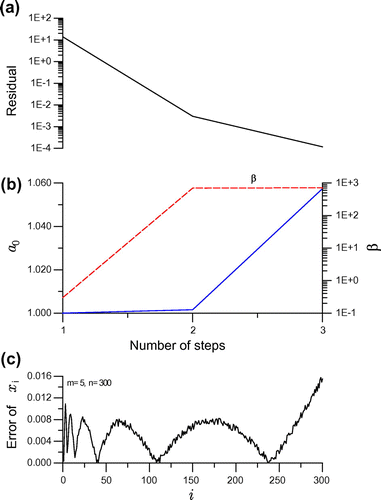
It is known that the condition number of Hilbert matrix grows as $e^{3.5n}$ when $n$ is very large. For the case with $n=300$, the condition number is extremely huge up to the order of ${10}^{522}$. We solve this problem by using the DODA with the Krylov subspace method. Under a noise $\mathit{\sigma }={10}^{-6}$, and for $n=300$ and $m=5$, the DODA is convergent very fast only through three steps with the convergence criterion $\mathit{\epsilon }={10}^{-3}$, where the maximum error is $0.0158$. It is very time saving because we only need to calculate the $5\times 5$ matrix ${\mathbf{C}}^{-1}$ three times, which is using the MCGM developed by Liu et al. [46]. 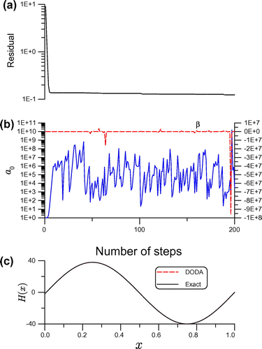Under a convergence criterion ${\mathit{\epsilon }}_1={10}^{-5}$ in Equation (7878 $$\begin{array}{c}\hfill \Vert {\mathbf{R}}_k\Vert <{\mathit{\epsilon }}_1,\end{array}$$78 ), the process to find $\mathbf{D}$ is convergent very fast with five or six iterations, although we do not show them at here. The numerical results are shown in Figure 1. It is interesting that even for a large value of $n=300$, we do not need a large value of $m$, of which merely $m=5$ was used. Also we can observe that the accuracy does not lose although the ill-posedness of the linear Hilbert problem is highly increased for $n=300$.

Figure 1. For example 1 solved by the DODA with Krylov subspace, showing (a) residual, (b) $a_0$ and $\mathit{\beta }$ and (c) numerical error.

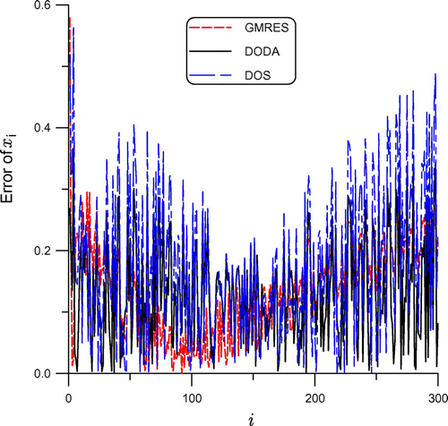
As mentioned, the algorithm in [19] is applied to solve linear problem by selecting a suitable value of $m$ for the dimension of the Krylov subspace. This algorithm has been named the DOS. Under a large noise with $\mathit{\sigma }=0.05$ and for $n=300$, we take $m=2$ and apply the GMRES, DODA and DOS to solve this problem, whose numerical errors are compared in Figure 2. The maximum error of DODA is $0.367$, while that for the GMRES is 0.579 and DOS is 0.566. The RMSE obtained by the DODA is 0.154, while that obtained by the GMRES is $0.16$, and that obtained by the DOS is 0.214. It can be seen that the DODA is slightly accurate than the GMRES and the DOS.

Figure 2. For example 1 under a large noise with $\mathit{\sigma }=0.05$, comparing numerical errors obtained by the DODA, DOS and GMRES.

6.2 Example 2

In this section, we apply the DODA to identify an unknown space-dependent heat source function $H(x)$ for a one-dimensional heat conduction equation:96 $$\begin{array}{cc}& u_t(x,t)=u_{xx}(x,t)+H(x),0<x<\ell ,0<t<t_f,\hfill \end{array}$$96 97 $$\begin{array}{cc}& u(0,t)=u_0(t),u(\ell ,t)=u_{\ell }(t),\hfill \end{array}$$97 98 $$\begin{array}{cc}& u(x,0)=f(x).\hfill \end{array}$$98 In order to identify $H(x)$, we can impose an extra condition:99 $$\begin{array}{c}\hfill u_x(0,t)=q(t).\end{array}$$99 We propose a numerical differential method by letting $v=u_t$. Taking the differentials of Equations (9696 $$\begin{array}{cc}& u_t(x,t)=u_{xx}(x,t)+H(x),0<x<\ell ,0<t<t_f,\hfill \end{array}$$96 ), (9797 $$\begin{array}{cc}& u(0,t)=u_0(t),u(\ell ,t)=u_{\ell }(t),\hfill \end{array}$$97 ) and (9999 $$\begin{array}{c}\hfill u_x(0,t)=q(t).\end{array}$$99 ) with respect to $t$, and letting $v=u_t$, we can derive100 $$\begin{array}{cc}& v_t(x,t)=v_{xx}(x,t),0<x<\ell ,0<t<t_f,\hfill \end{array}$$100 101 $$\begin{array}{cc}& v(0,t)={\dot{u}}_0(t),\hfill \end{array}$$101 102 $$\begin{array}{cc}& v(\ell ,t)={\dot{u}}_{\ell }(t),\hfill \end{array}$$102 103 $$\begin{array}{cc}& v_x(0,t)=\dot{q}(t).\hfill \end{array}$$103 This is an inverse heat conduction problem (IHCP) for $v(x,t)$ without using the initial condition.

Therefore, we can first solve the above IHCP for $v(x,t)$ by using the method of fundamental solutions (MFS) to obtain a linear equations system, and then the method introduced in Section 5 is used to solve the resultant linear equations system; hence, we can construct $u(x,t)$ by104 $$\begin{array}{c}\hfill u(x,t)={\int }_0^{t}v(x,\mathit{\xi })d\mathit{\xi }+f(x),\end{array}$$104 which automatically satisfies the initial condition in Equation (9898 $$\begin{array}{cc}& u(x,0)=f(x).\hfill \end{array}$$98 ).

From Equation (104104 $$\begin{array}{c}\hfill u(x,t)={\int }_0^{t}v(x,\mathit{\xi })d\mathit{\xi }+f(x),\end{array}$$104 ), it follows that105 $$\begin{array}{c}\hfill u_{xx}(x,t)={\int }_0^t{v}_{xx}(x,\mathit{\xi })d\mathit{\xi }+f^{″}(x),\end{array}$$105 which together with $u_t=v$ being inserted into Equation (9696 $$\begin{array}{cc}& u_t(x,t)=u_{xx}(x,t)+H(x),0<x<\ell ,0<t<t_f,\hfill \end{array}$$96 ) leads to106 $$\begin{array}{c}\hfill v(x,t)={\int }_0^t{v}_{xx}(x,\mathit{\xi })d\mathit{\xi }+f^{″}(x)+H(x).\end{array}$$106 Inserting Equation (100100 $$\begin{array}{cc}& v_t(x,t)=v_{xx}(x,t),0<x<\ell ,0<t<t_f,\hfill \end{array}$$100 ) for $v_{xx}=v_t$ into the above equation and integrating it, we can derive the following equation to recover $H(x)$:107 $$\begin{array}{c}\hfill H(x)=v(x,0)-f^{″}(x).\end{array}$$107 For the purpose of comparison, we consider the following exact solutions:108 $$\begin{array}{cc}& u(x,t)=x^2+2xt+sin(2\mathit{\pi }x),\hfill \\ & H(x)=2x-2+4{\mathit{\pi }}^{2}sin(2\mathit{\pi }x).\hfill \end{array}$$108 In Equation (107107 $$\begin{array}{c}\hfill H(x)=v(x,0)-f^{″}(x).\end{array}$$107 ), we disregard the ill-posedness of $f^{″}(x)$, and suppose that the data $f^{″}(x)$ are given exactly. A random noise with an intensity $\mathit{\sigma }=10\%$ is added on the data $\dot{q}(t)$. 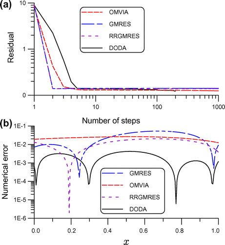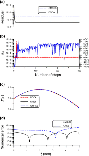Under the following parameters $m=10$ and $\mathit{\gamma }=0.25$, we solve this problem by the DODA with 200 steps. In Figure 3(a) and (b), we plot the residual, $a_0$ and $\mathit{\beta }$, and the numerical solution is compared with the exact solution in Figure 3(c). The numerical error is shown in Figure 4(b), whose maximum error is 0.00421. It can be seen that the present DODA can provide very accurate numerical result. This result is better than that calculated by Liu [47] using the vector regularization iterative method, whose maximum error is 0.0086. Then under the same parameters as that used in the DODA, we apply the GMRES,[17] the RRGMRES [40] and the OMVIA [24] to solve this problem. The residuals and numerical errors are compared in Figure 4. When the maximum error of GMRES is 0.053, the maximum error of RRGMRES is 0.02, and the maximum error of OMVIA is 0.0265. The maximum error of DODA as shown in the above is 0.00421, which is the best one among the four numerical methods. The RMSE of GMRES is $0.032$, the RMSE of RRGMRES is 0.014, the RMSE of OMVIA is 0.023 and the RMSE of DODA is 0.0024. It can be seen that the DODA is much accurate than other three numerical algorithms.

Figure 3. For example 2 solved by the DODA with Krylov subspace, showing (a) residual, (b) $a_0$ and $\mathit{\beta }$ and (c) numerical error.

Figure 4. For example 2 solved by the DODA, GMRES, RRGMRES and OMVIA, comparing (a) residuals and (b) numerical errors.

6.3 Example 3

When the backward heat conduction problem (BHCP) is considered in a spatial interval of $0<x<\ell$ by subjecting to the boundary conditions at two ends of a slab:109 $$\begin{array}{cc}& u_t(x,t)=\mathit{\kappa }{u}_{xx}(x,t),0<t<T,0<x<\ell ,\hfill \end{array}$$109 110 $$\begin{array}{cc}& u(0,t)=u_0(t),u(\ell ,t)=u_{\ell }(t),\hfill \end{array}$$110 we solve $u$ under a final time condition:111 $$\begin{array}{c}\hfill u(x,T)=u^T(x).\end{array}$$111 The fundamental solution of Equation (109109 $$\begin{array}{cc}& u_t(x,t)=\mathit{\kappa }{u}_{xx}(x,t),0<t<T,0<x<\ell ,\hfill \end{array}$$109 ) is given as follows:112 $$\begin{array}{c}\hfill K(x,t)=\frac{H(t)}{2\sqrt{\mathit{\kappa }\mathit{\pi }t}}exp\left(\frac{-x^2}{4\mathit{\kappa }t}\right),\end{array}$$112 where $H(t)$ is the Heaviside function.

The MFS has a serious drawback that the resulting linear equations system is always highly ill conditioned, when the number of source points is increased, or when the distances of source points are increased.

In the MFS, the solution of $u$ at the field point $\mathbf{z}=(x,t)$ can be expressed as a linear combination of the fundamental solutions $U(\mathbf{z},{\mathbf{s}}_j)$:113 $$\begin{array}{c}\hfill u(\mathbf{z})=\sum _{j=1}^n{c}_{j}U(\mathbf{z},{\mathbf{s}}_j),{\mathbf{s}}_j=({\mathit{\eta }}_j,{\mathit{\tau }}_j)\in {\mathrm{\Omega }}^c,\end{array}$$113 where $n$ is the number of source points, $c_j$ are unknown coefficients and ${\mathbf{s}}_j$ are source points being located in the complement ${\mathrm{\Omega }}^c$ of $\mathrm{\Omega }=[0,\ell ]\times [0,T]$. For the heat conduction equation, we have the basis functions114 $$\begin{array}{c}\hfill U(\mathbf{z},{\mathbf{s}}_j)=K(x-{\mathit{\eta }}_j,t-{\mathit{\tau }}_j).\end{array}$$114 It is known that the location of source points in the MFS has a great influence on the accuracy and stability. In a practical application of MFS to solve the BHCP, the source points are uniformly located on two vertical straight lines parallel to the $t$-axis, not over the final time, which was adopted by Hon and Li [48] and Liu [49], showing a large improvement than the line location of source points below the initial time. After imposing the boundary conditions and the final time condition to Equation (113113 $$\begin{array}{c}\hfill u(\mathbf{z})=\sum _{j=1}^n{c}_{j}U(\mathbf{z},{\mathbf{s}}_j),{\mathbf{s}}_j=({\mathit{\eta }}_j,{\mathit{\tau }}_j)\in {\mathrm{\Omega }}^c,\end{array}$$113 ), we can obtain a linear equations system:115 $$\begin{array}{c}\hfill \mathbf{B}\mathbf{x}=\mathbf{b},\end{array}$$115 where116 $$\begin{array}{cc}& B_{ij}=U({\mathbf{z}}_i,{\mathbf{s}}_j),\mathbf{x}={(c_1,\cdots ,c_n)}^{\text{T}},\hfill \\ & \mathbf{b}={(u_{\ell }(t_i),i=1,\dots ,m_1;u^T(x_j),j=1,\dots ,m_2;u_0(t_k),k=m_1,\dots ,1)}^{\text{T}},\hfill \end{array}$$116 and $n=2m_1+m_2$.

Since the BHCP is highly ill posed, the ill condition of the coefficient matrix $\mathbf{B}$ in Equation (115115 $$\begin{array}{c}\hfill \mathbf{B}\mathbf{x}=\mathbf{b},\end{array}$$115 ) is serious. To overcome the ill-posedness of Equation (115115 $$\begin{array}{c}\hfill \mathbf{B}\mathbf{x}=\mathbf{b},\end{array}$$115 ), we can use the DODA to solve this problem. Here, we compare the numerical solution with an exact solution:$$u(x,t)=cos(\mathit{\pi }x)exp(-{\mathit{\pi }}^{2}t).$$For the case with $T=1$, the value of final time data is in the order of ${10}^{-4}$, which is small by comparing with the value of the initial temperature $f(x)=u_0(x)=cos(\mathit{\pi }x)$ to be retrieved, which is $O(1)$. First we impose a relative random noise with an intensity $\mathit{\sigma }=10\%$ being imposed on the final time data. 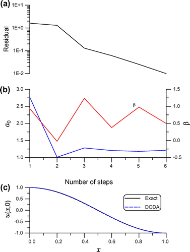Under the following parameters $m_1=15$, $m_2=8$, $m=16$, $\mathit{\gamma }=0.005$ and $\mathit{\epsilon }={10}^{-2}$ and ${\mathit{\epsilon }}_1={10}^{-8}$, we solve this problem by the DODA. With five steps the DODA is convergent. In Figure 5(a) and (b), we plot the residual, $a_0$ and $\mathit{\beta }$, and the numerical solution is compared with the exact solution in Figure 5(c), whose maximum error is $9.25\times {10}^{-3}$. It can be seen that the present DODA converges very fast and is very robust against noise, and we can provide a very accurate numerical result by using the DODA.

Figure 5. For example 3 solved by the DODA with Krylov subspace, showing (a) residual, (b) $a_0$ and $\mathit{\beta }$ and (c) comparing numerical and exact solutions.

Then under the same parameters as that used in the DODA, we also apply the GMRES,[17] the RRGMRES,[40] the OMVIA [24] and the OTVIA [13] to solve this problem. The residuals and numerical errors are compared in Figure 6. The OMVIA is convergent with 142 steps and the maximum error is 0.041. The GMRES is convergent with 16 steps and the maximum error is 0.148. The RRGMRES is convergent with four steps and the maximum error is 0.0124. The OTVIA does not converge within 1000 steps and the maximum error is 0.0994. Then we apply the DOS with $m=16$ to solve this problem, whose numerical error as shown in Figure 6(b) with the maximum error being $0.0194$ is better than that of GMRES, OMVIA and OTVIA, but is worse than that of DODA. It can be seen that the DODA is the best one among the six numerical methods, which is convergent faster and accurate than other five algorithms DOS, GMRES, RRGMRES, OMVIA and OTVIA. The RMSE of GMRES is $0.104$, the RMSE of DOS is $0.0136$, the RMSE of OMVIA is $0.0282$ and the RMSE of OTVIA is $0.0622$. The RMSE of DODA is $6.1\times {10}^{-3}$, while that for the RRGMRES is $7.9\times {10}^{-3}$. For this ill-posed problem, the DODA is better than the RRGMRES.

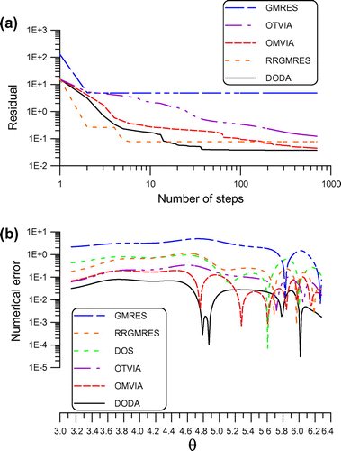
Figure 6. For example 3 solved by the DODA, DOS, GMRES, RRGMRES, OMVIA and OTVIA, comparing (a) residuals and (b) numerical errors.

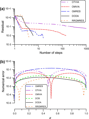
Figure 7. For example 4 solved by the DODA with Krylov subspace, showing (a) residual, (b) $a_0$ and $\mathit{\beta }$ and (c) comparing numerical and exact solutions.

Figure 8. For example 4 solved by the DODA, DOS, GMRES, RRGMRES, OMVIA and OTVIA, comparing (a) residuals and (b) numerical errors.

Figure 9. For example 5 solved by the DODA and GMRES, showing (a) residuals, (b) $a_0$ and $\mathit{\beta }$, (c) comparing numerical and exact solutions and (d) numerical errors.

6.4 Example 4

Let us consider the inverse Cauchy problem for the Laplace equation:117 $$\begin{array}{cc}& \mathrm{\Delta }u=u_{rr}+\frac{1}{r}{u}_r+\frac{1}{r^2}{u}_{\mathit{\theta }\mathit{\theta }}=0,\hfill \end{array}$$117 118 $$\begin{array}{cc}& u(\mathit{\rho },\mathit{\theta })=h(\mathit{\theta }),0\le \mathit{\theta }\le \mathit{\pi },\hfill \end{array}$$118 119 $$\begin{array}{cc}& u_n(\mathit{\rho },\mathit{\theta })=g(\mathit{\theta }),0\le \mathit{\theta }\le \mathit{\pi },\hfill \end{array}$$119 where $h(\mathit{\theta })$ and $g(\mathit{\theta })$ are given function. The inverse Cauchy problem is specified as follows:

To seek an unknown boundary function $f(\mathit{\theta })$ on the part ${\mathrm{\Gamma }}_2:=\{(r,\mathit{\theta })|r=\mathit{\rho }(\mathit{\theta }),\mathit{\pi }<\mathit{\theta }<2\mathit{\pi }\}$ of the boundary under Equations (117117 $$\begin{array}{cc}& \mathrm{\Delta }u=u_{rr}+\frac{1}{r}{u}_r+\frac{1}{r^2}{u}_{\mathit{\theta }\mathit{\theta }}=0,\hfill \end{array}$$117 )–(119119 $$\begin{array}{cc}& u_n(\mathit{\rho },\mathit{\theta })=g(\mathit{\theta }),0\le \mathit{\theta }\le \mathit{\pi },\hfill \end{array}$$119 ) with the overspecified data being given on ${\mathrm{\Gamma }}_1:=\{(r,\mathit{\theta })|r=\mathit{\rho }(\mathit{\theta }),0\le \mathit{\theta }\le \mathit{\pi }\}$.

It is well known that the MFS can be used to solve the Laplace equation when a fundamental solution is known. In the MFS, the solution of $u$ at the field point $\mathbf{x}=(rcos\mathit{\theta },rsin\mathit{\theta })$ can be expressed as a linear combination of fundamental solutions $U(\mathbf{x},{\mathbf{s}}_j)$:120 $$\begin{array}{c}\hfill u(\mathbf{x})=\sum _{j=1}^n{c}_{j}U(\mathbf{x},{\mathbf{s}}_j),{\mathbf{s}}_j\in {\mathrm{\Omega }}^c.\end{array}$$120 For the Laplace equation (117117 $$\begin{array}{cc}& \mathrm{\Delta }u=u_{rr}+\frac{1}{r}{u}_r+\frac{1}{r^2}{u}_{\mathit{\theta }\mathit{\theta }}=0,\hfill \end{array}$$117 ), we have the fundamental solutions:121 $$\begin{array}{c}\hfill U(\mathbf{x},{\mathbf{s}}_j)=ln{r}_j,r_j=\Vert \mathbf{x}-{\mathbf{s}}_j\Vert .\end{array}$$121 In the practical application of MFS, by imposing the boundary conditions (118118 $$\begin{array}{cc}& u(\mathit{\rho },\mathit{\theta })=h(\mathit{\theta }),0\le \mathit{\theta }\le \mathit{\pi },\hfill \end{array}$$118 ) and (119119 $$\begin{array}{cc}& u_n(\mathit{\rho },\mathit{\theta })=g(\mathit{\theta }),0\le \mathit{\theta }\le \mathit{\pi },\hfill \end{array}$$119 ) at $N$ points on Equation (120120 $$\begin{array}{c}\hfill u(\mathbf{x})=\sum _{j=1}^n{c}_{j}U(\mathbf{x},{\mathbf{s}}_j),{\mathbf{s}}_j\in {\mathrm{\Omega }}^c.\end{array}$$120 ), we can obtain a linear equations system:122 $$\begin{array}{c}\hfill \mathbf{B}\mathbf{c}=\mathbf{b},\end{array}$$122 where123 $$\begin{array}{cc}& {\mathbf{x}}_i=(x_i^1,x_i^2)=(\mathit{\rho }({\mathit{\theta }}_i)cos{\mathit{\theta }}_i,\mathit{\rho }({\mathit{\theta }}_i)sin{\mathit{\theta }}_i),\hfill \\ & {\mathbf{s}}_j=(s_j^1,s_j^2)=(R({\mathit{\theta }}_j)cos{\mathit{\theta }}_j,R({\mathit{\theta }}_j)sin{\mathit{\theta }}_j),\hfill \\ & B_{ij}=ln\Vert {\mathbf{x}}_i-{\mathbf{s}}_j\Vert ,\text{if}i\text{is odd},\hfill \\ & B_{ij}=\frac{\mathit{\eta }({\mathit{\theta }}_i)}{\Vert {\mathbf{x}}_i-{\mathbf{s}}_j{\Vert }^2}\hfill \\ & \times \left(\mathit{\rho },({\mathit{\theta }}_i),-,s_j^1,cos,{\mathit{\theta }}_i,-,s_j^2,sin,{\mathit{\theta }}_i,-,\frac{{\mathit{\rho }}^{\prime }({\mathit{\theta }}_i)}{\mathit{\rho }({\mathit{\theta }}_i)},[s_j^{1}sin{\mathit{\theta }}_i-s_j^{2}cos{\mathit{\theta }}_i]\right),\text{if}i\text{is even},\hfill \\ & \mathbf{c}={(c_1,\dots ,c_n)}^{\text{T}},\mathbf{b}={(h({\mathit{\theta }}_1),g({\mathit{\theta }}_1),\dots ,h({\mathit{\theta }}_N),g({\mathit{\theta }}_N))}^{\text{T}},\hfill \end{array}$$123 in which $n=2N$, and124 $$\begin{array}{c}\hfill \mathit{\eta }(\mathit{\theta })=\frac{\mathit{\rho }(\mathit{\theta })}{\sqrt{{\mathit{\rho }}^2(\mathit{\theta })+{[{\mathit{\rho }}^{\prime }(\mathit{\theta })]}^2}}.\end{array}$$124 The above $R(\mathit{\theta })=\mathit{\rho }(\mathit{\theta })+D$ with an offset $D$ can be used to locate the source points along a contour with a radius $R(\mathit{\theta })$.

For the purpose of comparison, we consider the following exact solution:125 $$\begin{array}{c}\hfill u(x,y)=cosxcoshy+sinxsinhy,\end{array}$$125 defined in a domain with a complex amoeba-like irregular shape as a boundary:126 $$\begin{array}{c}\hfill \mathit{\rho }(\mathit{\theta })=exp(sin\mathit{\theta }){sin}^2(2\mathit{\theta })+exp(cos\mathit{\theta }){cos}^2(2\mathit{\theta }).\end{array}$$126 After imposing the boundary conditions (118118 $$\begin{array}{cc}& u(\mathit{\rho },\mathit{\theta })=h(\mathit{\theta }),0\le \mathit{\theta }\le \mathit{\pi },\hfill \end{array}$$118 ) and (119119 $$\begin{array}{cc}& u_n(\mathit{\rho },\mathit{\theta })=g(\mathit{\theta }),0\le \mathit{\theta }\le \mathit{\pi },\hfill \end{array}$$119 ) at $N$ points on Equation (120120 $$\begin{array}{c}\hfill u(\mathbf{x})=\sum _{j=1}^n{c}_{j}U(\mathbf{x},{\mathbf{s}}_j),{\mathbf{s}}_j\in {\mathrm{\Omega }}^c.\end{array}$$120 ), we can obtain a linear equations system. The noise being imposed on the measured data $h$ and $g$ is $\mathit{\sigma }=0.01$.

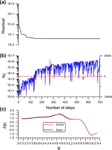
We solve this problem by the DODA with $m=5$ and $\mathit{\gamma }=0.2$. The descent direction $\mathbf{u}$ is solved from ${\mathbf{B}}^{\text{T}}\mathbf{B}\mathbf{u}={\mathbf{B}}^{\text{T}}\mathbf{r}$. Through 700 steps the residual and the values of $a_0$ and $\mathit{\beta }$ are shown in Figure 7(a) and (b). The numerical solution and exact solution are compared in Figure 7(c), whose maximum error is smaller than 0.0884. It can be seen that the DODA can accurately recover the unknown boundary condition.

Then under the same parameters as that used in the DODA, we apply the GMRES,[17] the RRGMRES,[40] and the OMVIA [24] to solve this problem. The residuals and numerical errors are compared in Figure 8. When the maximum error of GMRES is 5.02 (failure) and the maximum error of RRGMRES is 1.16, the maximum error of OMVIA is 0.197. The maximum error of DODA as shown in the above is much better than that calculated by Liu [13] by using the OTVIA, of which the maximum error is 0.34. Then we apply the DOS with $m=10$ to solve this problem, whose numerical error as shown in Figure 8(b) with the maximum error being $0.955$ is better than that of GMRES, but is worse than that of RRGMRES, OMVIA, OTVIA and DODA. The RMSE of GMRES is $3.03$, the RMSE of RRGMRES is $0.553$, the RMSE of DOS is $0.602$, the RMSE of OMVIA is $0.127$ and the RMSE of OTVIA is $0.177$. The RMSE of DODA is $0.045$, which is better than other five algorithms. Again, it can be seen that the DODA is the best one among the six numerical methods, which is convergent faster and much more accurate than other five algorithms.

6.5 Example 5

Let us consider the following inverse problem to recover the external force $F(t)$ for127 $$\begin{array}{c}\hfill \ddot{y}(t)+\dot{y}(t)+y(t)=F(t).\end{array}$$127 In a time interval of $t\in [0,t_f]$, the discretized data $y_i=y(t_i)$ are supposed to be measurable, which are subjected to the random noise with an intensity $\mathit{\sigma }=0.01$. Usually, it is very difficult to recover the external force $F(t_i)$ from Equation (127127 $$\begin{array}{c}\hfill \ddot{y}(t)+\dot{y}(t)+y(t)=F(t).\end{array}$$127 ) by the direct differentials of the noisy data of displacements, because the differential is an ill-posed linear operator.

To approach this inverse problem by the polynomial interpolation, we begin with128 $$\begin{array}{c}\hfill p_m(x)=c_0+\sum _{k=1}^m{c}_k{x}^k.\end{array}$$128 Now, the coefficient $c_k$ is split into two coefficients $a_k$ and $b_k$ to absorb more interpolation points; in the meanwhile, $cos(k{\mathit{\theta }}_k)$ and $sin(k{\mathit{\theta }}_k)$ are introduced to reduce the condition number of the coefficient matrix. We suppose that129 $$\begin{array}{c}\hfill c_k=\frac{a_{k}cos(k{\mathit{\theta }}_k)}{R_{2k}^k}+\frac{b_{k}sin(k{\mathit{\theta }}_k)}{R_{2k+1}^k},\end{array}$$129 and130 $$\begin{array}{c}\hfill {\mathit{\theta }}_k=\frac{2k\mathit{\pi }}{m},k=1,\dots ,m.\end{array}$$130 The problem domain is $[a,b]$, and the interpolating points are:131 $$\begin{array}{c}\hfill a=x_0<x_1<x_2<\dots <x_{2m-1}<x_{2m}=b.\end{array}$$131 Substituting Equation (129129 $$\begin{array}{c}\hfill c_k=\frac{a_{k}cos(k{\mathit{\theta }}_k)}{R_{2k}^k}+\frac{b_{k}sin(k{\mathit{\theta }}_k)}{R_{2k+1}^k},\end{array}$$129 ) into Equation (128128 $$\begin{array}{c}\hfill p_m(x)=c_0+\sum _{k=1}^m{c}_k{x}^k.\end{array}$$128 ), we can obtain132 $$\begin{array}{c}\hfill p(x)=a_0+\sum _{k=1}^m\left[a_k,{\left(\frac{x}{R_{2k}}\right)}^k,cos,(k{\mathit{\theta }}_k),+,b_k,{\left(\frac{x}{R_{2k+1}}\right)}^k,sin,(k{\mathit{\theta }}_k)\right],\end{array}$$132 where we let $c_0=a_0$. Here, $a_k$ and $b_k$ are unknown coefficients. In order to obtain them, we impose the following $n$ interpolated conditions:133 $$\begin{array}{c}\hfill p(x_i)=y_i,i=0,\dots ,n-1.\end{array}$$133 Thus, we obtain a linear equations system to determine $a_k$ and $b_k$:134 $$\begin{array}{c}\hfill \left[\begin{array}{cccccc}1& \frac{x_{0}cos{\mathit{\theta }}_1}{R_2}& \frac{x_{0}sin{\mathit{\theta }}_1}{R_3}& \dots & {\left(\frac{x_0}{R_{2m}}\right)}^{m}cosm{\mathit{\theta }}_m& {\left(\frac{x_0}{R_{2m+1}}\right)}^{m}sinm{\mathit{\theta }}_m\\ [1ex]1& \frac{x_{1}cos{\mathit{\theta }}_1}{R_2}& \frac{x_{1}sin{\mathit{\theta }}_1}{R_3}& \dots & {\left(\frac{x_1}{R_{2m}}\right)}^{m}cosm{\mathit{\theta }}_m& {\left(\frac{x_1}{R_{2m+1}}\right)}^{m}sinm{\mathit{\theta }}_m\\ [1ex]⋮& ⋮& ⋮& ⋮& ⋮& ⋮\\ 1& \frac{x_{2m-1}cos{\mathit{\theta }}_1}{R_2}& \frac{x_{2m-1}sin{\mathit{\theta }}_1}{R_3}& \dots & {\left(\frac{x_{2m-1}}{R_{2m}}\right)}^{m}cosm{\mathit{\theta }}_m& {\left(\frac{x_{2m-1}}{R_{2m+1}}\right)}^{m}sinm{\mathit{\theta }}_m\\ [1ex]1& \frac{x_{2m}cos{\mathit{\theta }}_1}{R_2}& \frac{x_{2m}sin{\mathit{\theta }}_1}{R_3}& \dots & {\left(\frac{x_{2m}}{R_{2m}}\right)}^{m}cosm{\mathit{\theta }}_m& {\left(\frac{x_{2m}}{R_{2m+1}}\right)}^{m}sinm{\mathit{\theta }}_m\end{array}\right]\left[\begin{array}{c}{a}_0\\ a_1\\ b_1\\ ⋮\\ a_m\\ b_m\end{array}\right]=\left[\begin{array}{c}{y}_0\\ y_1\\ y_2\\ ⋮\\ y_{2m-1}\\ y_{2m}\\ \end{array}\right].\end{array}$$134 We note that the norm of the first column of the above coefficient matrix is $\sqrt{2m+1}$. According to the concept of equilibrated matrix,[50] we can derive the optimal scales for the current interpolation with a half-order technique as135 $$\begin{array}{cc}& R_{2k}={\mathit{\beta }}_0{\left(\frac{1}{2m+1},\sum _{j=0}^{2m},x_j^{2k},{(cosk{\mathit{\theta }}_k)}^2\right)}^{1/(2k)},k=1,2,\dots ,m,\hfill \end{array}$$135 136 $$\begin{array}{cc}& R_{2k+1}={\mathit{\beta }}_0{\left(\frac{1}{2m+1},\sum _{j=0}^{2m},x_j^{2k},{(sink{\mathit{\theta }}_k)}^2\right)}^{1/(2k)},k=1,2,\dots ,m,\hfill \end{array}$$136 where ${\mathit{\beta }}_0$ is a scaling factor.[50] The improved method uses $m$-order polynomial to interpolate $n=2m+1$ data nodes, while regular method with a full-order can only interpolate $m+1$ data points.

Now we fix $m_0=25$ (of the above $m$) and $t_f=5$ and consider the exact solution to be $F(t)=\mathit{\omega }cos(\mathit{\omega }t)+(1-{\mathit{\omega }}^2)sin(\mathit{\omega }t)$, which is obtained by inserting the exact value of $y(t)=sin(\mathit{\omega }t)$ into Equation (127127 $$\begin{array}{c}\hfill \ddot{y}(t)+\dot{y}(t)+y(t)=F(t).\end{array}$$127 ). The parameters used are $\mathit{\omega }=0.5$, and ${\mathit{\beta }}_0=2$. When we use the DODA with $m=4$, we let it run 300 steps. The descent direction $\mathbf{u}$ is solved from ${\mathbf{B}}^{\text{T}}\mathbf{B}\mathbf{u}={\mathbf{B}}^{\text{T}}\mathbf{r}$. The residual and the values of $a_0$ and $\mathit{\beta }$ are shown in Figure 9(a) and (b). The numerical solution and exact solution are compared in Figure 9(c), whose maximum error is smaller than 0.027. It can be seen that the DODA can accurately recover the unknown external force.

When we apply the GMRES to solve this problem, the parameter ${\mathit{\beta }}_0$ is changed to ${\mathit{\beta }}_0=6$, and the other parameters are unchanged. In Figure 9, we plot the results obtained by the GMRES with dashed-dotted lines, of which as shown in Figure 9(c) and (d) we can see that the GMRES is less accurate with the maximum error being 0.35. The RMSE obtained by the DODA is $1.14\times {10}^{-2}$, while that obtained by the GMRES is 0.117. It can be seen that the DODA is much accurate than the GMRES.

7 Conclusions and discussion

In the present paper, we have derived a double optimal algorithm, including an $m$-vector optimal search direction in an $m$-dimensional affine Krylov subspace to solve a highly ill-posed linear system. This algorithm is a multi-vector DODA, of which the expansion coefficients in the descent direction are solved in closed-form through double optimizations of two basic merit functions to measure the distance between $\mathbf{v}=\mathbf{B}\mathbf{u}$ and $\mathbf{r}$. The DODA has a good computational efficiency and accuracy in solving the ill-posed linear equations system. Numerical tests on the linear inverse problems have confirmed the robustness of the DODA against noisy disturbance even with an intensity being large up to $10\%$. For the test examples, we found that the DODA can converge fast and stable with the iterations account smaller than the dimension of the considered problem. As the usual Krylov subspace method, the value of $m$ cannot be too large; otherwise, many computational time is required to construct the Krylov matrix by the Arnoldi process at each iteration step. When $m$ is large, the Krylov matrix will be highly ill conditioned for the ill-posed problem. The DODA is convergent faster than other numerical methods investigated in this paper, and indeed it can achieve smaller residual errors than the GMRES, the RRGMRES and the OMVIA under the same value of $m$. In the proof of the convergence of the DODA, we have derived an exact equation to estimate the difference of two consecutive square residual norms:$$\Vert {\mathbf{r}}_{k+1}{\Vert }^2={\Vert {\mathbf{r}}_k\Vert }^2-\left[{\mathbf{r}}_k^{\text{T}},\mathbf{E},{\mathbf{r}}_k,+,\frac{{[{\mathbf{r}}_k^{\text{T}}({\mathbf{I}}_n-\mathbf{E})\mathbf{B}{\mathbf{r}}_k]}^2}{{\mathbf{r}}_k^{\text{T}}{\mathbf{B}}^{\text{T}}({\mathbf{I}}_n-\mathbf{E})\mathbf{B}{\mathbf{r}}_k}\right].$$How to maximize the quantity in the square brackets, i.e.$$max\left[{\mathbf{r}}_k^{\text{T}},\mathbf{E},{\mathbf{r}}_k,+,\frac{{[{\mathbf{r}}_k^{\text{T}}({\mathbf{I}}_n-\mathbf{E})\mathbf{B}{\mathbf{r}}_k]}^2}{{\mathbf{r}}_k^{\text{T}}{\mathbf{B}}^{\text{T}}({\mathbf{I}}_n-\mathbf{E})\mathbf{B}{\mathbf{r}}_k}\right]$$might be an important issue, which will lead to a further study of the structure of the Krylov subspace resulting to the best configuration of the projection operator $\mathbf{E}$. On the other hand, based on Theorem 5 in [20], the square residual obtained by the DODA is smaller than that obtained by the algorithms based on the least square of residual with the following relation:$$\Vert {\mathbf{r}}_k{\Vert }_{\text{DODA}}^2={\Vert {\mathbf{r}}_k\Vert }_{\text{LS}}^2-\frac{{[{\mathbf{r}}_k^{\text{T}}({\mathbf{I}}_n-\mathbf{E})\mathbf{B}{\mathbf{r}}_k]}^2}{{\mathbf{r}}_k^{\text{T}}{\mathbf{B}}^{\text{T}}({\mathbf{I}}_n-\mathbf{E})\mathbf{B}{\mathbf{r}}_k}.$$This fact revealed that the DODA is more efficient than other algorithms, and all numerical examples investigated in this paper by assessing the convergence speed, the maximum error, the absolute error and the RMSE confirmed the superiority of DODA.

Acknowledgments

The author highly appreciates the constructive comments from anonymous referees, which improve the quality of this paper. Highly appreciated are the project NSC-102-2221-E-002-125-MY3 and the 2011 Outstanding Research Award from the National Science Council of Taiwan, and the 2011 Taiwan Research Front Award from Thomson Reuters. It is also acknowledged that the author has been promoted as being a Lifetime Distinguished Professor of National Taiwan University since 2013.

References

- Stewart G. Introduction to matrix computations. New York (NY): Academic Press; 1973.
- Kunisch K, Zou J. Iterative choices of regularization parameters in linear inverse problems. Inverse Probl. 1998;14:1247–1264.
- Wang Y, Xiao T. Fast realization algorithms for determining regularization parameters in linear inverse problems. Inverse Probl. 2001;17:281–291.
- Xie J, Zou J. An improved model function method for choosing regularization parameters in linear inverse problems. Inverse Probl. 2002;18:631–643.
- Resmerita E. Regularization of ill-posed problems in Banach spaces: convergence rates. Inverse Probl. 2005;21:1303–1314.
- Chehab JP, Laminie J. Differential equations and solution of linear systems. Numer. Algorithms. 2005;40:103–124.
- Helmke U, Moore JB. Optimization and dynamical systems. Berlin: Springer; 1994.
- Liu CS. Optimally generalized regularization methods for solving linear inverse problems. CMC: Comput. Mater. Con. 2012;29:103–127.
- Liu CS. Scaled vector regularization method to solve ill-posed linear problems. Appl. Math. Comput. 2012;218:10602–10616.
- Liu CS. A dynamical Tikhonov regularization for solving ill-posed linear algebraic systems. Acta Appl. Math. 2012;123:285–307.
- Liu CS. An optimal preconditioner with an alternate relaxation parameter used to solve ill-posed linear problems. CMES: Comput. Model. Eng. Sci. 2013;92:241–269.
- Liu CS. A globally optimal iterative algorithm to solve an ill-posed linear system. CMES: Comput. Model. Eng. Sci. 2012;84:383–403.
- Liu CS. An optimal tri-vector iterative algorithm for solving ill-posed linear inverse problems. Inverse Probl. Sci. Eng. 2013;21:650–681.
- Liu CS. A globally optimal tri-vector method to solve an ill-posed linear system. J. Comput. Appl. Math. 2014;260:18–35.
- Barzilai J, Borwein JM. Two point step size gradient methods. IMA J. Numer. Anal. 1988;8:141–148.
- Akaike H. On a successive transformation of probability distribution and its application to the analysis of the optimum gradient method. Ann. Inst. Stat. Math. Tokyo. 1959;11:1–16.
- Saad Y, Schultz MH. GMRES: a generalized minimal residual algorithm for solving nonsymmetric linear systems. SIAM J. Sci. Stat. Comput. 1986;7:856–869.
- Liu CS, Atluri SN. An iterative method using an optimal descent vector, for solving an ill-conditioned system Bx = b, better and faster than the conjugate gradient method. CMES: Comput. Model. Eng. Sci. 2011;80:275–298.
- Liu CS. A doubly optimized solution of linear equations system expressed in an affine Krylov subspace. J. Comput. Appl. Math. 2014;260:375–394.
- Liu CS. Discussing a more fundamental concept than the minimal residual method for solving linear system in a Krylov subspace. J. Math. Res. 2013;5:58–70.
- Liu CS. An optimally generalized steepest-descent algorithm for solving ill-posed linear systems. J. Appl. Math. 2013; ID 154358, 15 p.
- Jacoby SLS, Kowalik JS, Pizzo JT. Iterative methods for nonlinear optimization problems. New Jersey (NJ): Prentice-Hall; 1972.
- Ostrowski AM. Solution of equations in Euclidean and Banach spaces. 3rd ed. New York (NY): Academic Press; 1973.
- Liu CS. An optimal multi-vector iterative algorithm in a Krylov subspace for solving the ill-posed linear inverse problems. CMC: Comput. Mater. Con. 2013;33:175–198.
- Dongarra J, Sullivan F. Guest editors’ introduction to the top 10 algorithms. Comput. Sci. Eng. 2000;2:22–23.
- Simoncini V, Szyld DB. Recent computational developments in Krylov subspace methods for linear systems. Numer. Linear Algebra Appl. 2007;14:1–59.
- Saad Y. Krylov subspace methods for solving large unsymmetric linear systems. Math. Comput. 1981;37:105–126.
- Freund RW, Nachtigal NM. QMR: a quasi-minimal residual method for non-Hermitian linear systems. Numer. Math. 1991;60:315–339.
- van Den Eshof J, Sleijpen GLG. Inexact Krylov subspace methods for linear systems. SIAM J. Matrix Anal. Appl. 2004;26:125–153.
- Hestenes MR, Stiefel EL. Methods of conjugate gradients for solving linear systems. J. Res. Nat. Bur. Stand. 1952;49:409–436.
- Lanczos C. Solution of systems of linear equations by minimized iterations. J. Res. Nat. Bur. Stand. 1952;49:33–53.
- Paige CC, Saunders MA. Solution of sparse indefinite systems of linear equations. SIAM J. Numer. Anal. 1975;12:617–629.
- Fletcher R. Conjugate gradient methods for indefinite systems. Lecture notes in Math. Vol. 506. Berlin: Springer-Verlag; 1976. p. 73–89.
- Sonneveld P. CGS: a fast Lanczos-type solver for nonsymmetric linear systems. SIAM J. Sci. Stat. Comput. 1989;10:36–52.
- van der Vorst HA. Bi-CGSTAB: a fast and smoothly converging variant of Bi-CG for the solution of nonsymmetric linear systems. SIAM J. Sci. Stat. Comput. 1992;13:631–644.
- Saad Y, van der Vorst HA. Iterative solution of linear systems in the 20th century. J. Comput. Appl. Math. 2000;123:1–33.
- Saad Y. Iterative methods for sparse linear systems. 2nd ed. Pennsylvania (PA): SIAM; 2003.
- van der Vorst HA. Iterative Krylov methods for large linear systems. New York (NY): Cambridge University Press; 2003.
- Liu CS. The concept of best vector used to solve ill-posed linear inverse problems. CMES: Comput. Model. Eng. Sci. 2012;83:499–525.
- Calvetti C, Lewis B, Reichel L. GMRES-type methods for inconsistent systems. Linear Algebra Appl. 2000;316:157–169.
- Kuroiwa N, Nodera T. A note on the GMRES method for linear discrete ill-posed problems. Adv. Appl. Math. Mech. 2009;1:816–829.
- Matinfar M, Zareamoghaddam H, Eslami M, Saeidy M. GMRES implementations and residual smoothing techniques for solving ill-posed linear systems. Comput. Math. Appl. 2012;63:1–13.
- Morikuni K, Reichel L, Hayami K. FGMRES for linear discrete ill-posed problems. Appl. Numer. Math. 2014;75:175–187.
- Yin JF, Hayami K. Preconditioned GMRES methods with incomplete Givens orthogonalization method for large sparse least-squares problems. J. Comput. Appl. Math. 2009;226:177–186.
- Horn RA, Johnson CR. Matrix analysis. New York (NY): Cambridge University Press; 1985.
- Liu CS, Hong HK, Atluri SN. Novel algorithms based on the conjugate gradient method for inverting ill-conditioned matrices, and a new regularization method to solve ill-posed linear systems. CMES: Comput. Model. Eng. Sci. 2010;60:279–308.
- Liu CS. A vector regularization method to solve linear inverse problems. Inverse Probl. Sci. Eng. 2013. dx.doi.org/10.1080/17415977.2013.823415.
- Hon YC, Li M. A discrepancy principle for the source points location in using the MFS for solving the BHCP. Int. J. Comput. Methods. 2009;6:181–197.
- Liu CS. The method of fundamental solutions for solving the backward heat conduction problem with conditioning by a new post-conditioner. Numer. Heat Transfer B: Fundam. 2011;60:57–72.
- Liu CS. A two-side equilibration method to reduce the condition number of an ill-posed linear system. CMES: Comput. Model. Eng. Sci. 2013;91:17–42.