Comparative numerical analysis of identification problems related to nonlinear transport-diffusion model of a settler

Abstract

Identification problems related to age dependent models of a settling process in the secondary settler of a wastewater treatment plant are considered. The basic model is governed by the nonlinear parabolic equation $u_t(x,t)=-div(Q(x,t;c(x))u(x,t)-D(x)u_x(x,t))$ describing the scalar conservation law for the density of sludge mass, and by a nonlocal (integral form) additional condition. The problem is formulated as an identification problem, where the sludge concentration $c(x)$ is assumed to be a control. The mathematical analysis, based on the weak solution theory of PDEs, of the basic model shows the degree of sensitivity of the solution $u(x,t)$ of the parabolic equation with respect to the coefficient $c(x)$. The results obtained here are then applied to two widely accepted settling velocity models ($Q(x,t;c(x))=\mathit{\nu }(t)c(x)$ and $Q(x,t;c(x))={\mathit{\nu }}_{0}exp(-{\mathit{\alpha }}_{0}c(x)$). An effective iteration algorithm for numerical solution of identification problems related to these models is proposed. The algorithm is tested for the both settling velocity models. Computational simulation permits one to show an influence of the settling velocity models to the behavior of the sludge concentration $c(x)$.

Keywords:

• settling velocity models
• nonlinear transport-diffusion equation
• identification problem
• sensitivity analysis
• nonlocal (integral form) additional condition

1 Introduction

The paper deals with the estimation of the sludge concentration in the secondary settler, which is designed to substantially degrade the biological content of the sewage which are derived from human waste, food waste, soaps and detergent, etc. of a wastewater treatment plant. Figure 1 shows a generalized schematic outline of an wastewater treatment process in the plant. Most engineering literature is devoted to pure experimental studies, with analysis of various data measured for concrete settling process or real plant.[1] Notwithstanding the importance of these experimental studies, during last decades the number of theoretical studies related to settling process in a wastewater treatment increases. Thus, an analytical model using partial differential equations expressing the sludge mass conservation is proposed in [2]. A layered cylindrical settler model, expressing the sludge mass conservation and allowing to calculate the sludge concentration in each layer from one time step to another one, is studied by [3, 4]. Depending on the nature and concentration of solid particles, classification of various settling characteristics in wastewater treatment plant are presented in [4]. Most of subsequent settling models are still using this classification. Another kind of mathematical models are based on more general approach, and can be used for general settler. These kinds of mathematical models are proposed in [5], and then developed in [6–8]. The mathematical model proposed here can be considered as an extension of the model given in [9]. Specifically, we study the following transport-diffusion identification model of a settler, with nonlocal condition:1 $$\begin{array}{c}\hfill \left\{\begin{array}{cc}{u}_t(x,t)={(D(x)u_x(x,t))}_x-{(V(x,t;c(x))u(x,t))}_x,\forall (x,t)\in \mathbb{R}\times {\mathbb{R}}_{+},\hfill & \\ u(x,0)=\mathit{\phi }(x),\forall x\in \mathbb{R},\hfill & \\ {\int }_0^{\infty }u(x,t)dt=c(x),\forall x\in \mathbb{R}.\hfill \end{array}\right.\end{array}$$1 Here the density of sludge particles having spent time $t\in (0,\infty )$ in a settler at point $x\in (-\infty ,\infty )$ is defined by the function $u=u(x,t)$. The function $c(x)$ denotes the sludge concentration at point $x$. This model assumes that the mass transport is due to not only advection, but also diffusion $D(x)>0$. The settling mechanism is modeled by the function $V=V(x,t;c(x))$, which usually includes the water velocity, and settling velocity. The later depends on the sludge concentration $c(x)$ also. In the simplest case, when $V={\mathit{\nu }}_{0}c(x)$, and the maximum settling velocity ${\mathit{\nu }}_0>0$ is a constant, the above transport-diffusion model has been considered in [10]. It is shown here that in this case the PDE model can be reduced to a nonlinear ODE model. When2 $$\begin{array}{c}\hfill V(x,t;c(x)):=\mathit{\nu }(t)c(x),\end{array}$$2 and the settling velocity $\mathit{\nu }(t)$ depends on time, another kind of mathematical models arise in convective-diffusive fluid problems.[11] In subsequent, we will define this model, governed by Equations (11 $$\begin{array}{c}\hfill \left\{\begin{array}{cc}{u}_t(x,t)={(D(x)u_x(x,t))}_x-{(V(x,t;c(x))u(x,t))}_x,\forall (x,t)\in \mathbb{R}\times {\mathbb{R}}_{+},\hfill & \\ u(x,0)=\mathit{\phi }(x),\forall x\in \mathbb{R},\hfill & \\ {\int }_0^{\infty }u(x,t)dt=c(x),\forall x\in \mathbb{R}.\hfill \end{array}\right.\end{array}$$1 ) and (22 $$\begin{array}{c}\hfill V(x,t;c(x)):=\mathit{\nu }(t)c(x),\end{array}$$2 ), as the Model A.

Figure 1. A schematic outline of an wastewater treatment plant.

One of the most widely accepted settling velocity model is proposed in [12]:3 $$\begin{array}{c}\hfill V(x,t;c(x)):={\mathit{\nu }}_{0}exp(-{\mathit{\alpha }}_{0}c(x)),\end{array}$$3 where ${\mathit{\nu }}_0>0$ is the maximum settling velocity, and ${\mathit{\alpha }}_0>0$ is the model parameter. This settling velocity model has successfully been used in [4, 13, 14]. We will define this model which uses the Vesilind model of settling mechanism, as the Model B. This model is governed by Equations (11 $$\begin{array}{c}\hfill \left\{\begin{array}{cc}{u}_t(x,t)={(D(x)u_x(x,t))}_x-{(V(x,t;c(x))u(x,t))}_x,\forall (x,t)\in \mathbb{R}\times {\mathbb{R}}_{+},\hfill & \\ u(x,0)=\mathit{\phi }(x),\forall x\in \mathbb{R},\hfill & \\ {\int }_0^{\infty }u(x,t)dt=c(x),\forall x\in \mathbb{R}.\hfill \end{array}\right.\end{array}$$1 ) and (33 $$\begin{array}{c}\hfill V(x,t;c(x)):={\mathit{\nu }}_{0}exp(-{\mathit{\alpha }}_{0}c(x)),\end{array}$$3 ).

Besides of the above cited studies, various mathematical models related to the convection-diffusion equation have been considered in [15–18]. Some of these mathematical models also lead to inverse/identification problems with local or nonlocal additional conditions (see [15] and references therein). Note that when the coefficient $c(x)$ is known, the first two equations in (1) define the linear direct problem. However, when the $c(x)$ is unknown and needs to be defined from the last integral condition in (1), then the identification problem (1) is nonlinear.

This study is motivated by computer simulation of the secondary settling process based on the above mathematical models. Our goal is to estimate an influence of existing settling velocity models/parameters to the behavior of the sludge concentration function $c(x)$.

The paper is organized as follows. The sensitivity analysis of the solution $u(x,t)$ of the parabolic problem with respect to the coefficient $c(x)$ is discussed in Section 2. Iteration algorithm and numerical results for the Model A and Model B, are given in Sections 3 and 4, respectively. In Section 5 a computational comparative analysis of both models is presented. This analysis shows similarity as well as differences of two models, also permits one to estimate an influence of Vesilind parameters to the behavior of the sludge concentration coefficient $c(x)$.

2 Sensitivity analysis of the solution $u(x,t)$ with respect to the coefficient $c(x)$

We suppose that $u(x,t)\to 0,|x|\to \infty$, and $u(x,t)\to 0,t\to \infty$ in (1) and consider the parabolic problem4 $$\begin{array}{c}\hfill \left\{\begin{array}{c}{u}_t={(D(x)u_x)}_x-\mathit{\nu }(t){(Q(c(x),t)u)}_x,(x,t)\in {\mathrm{\Omega }}_T,\hfill \\ u(-L,t)=u(L,t)=0,\forall t\in (0,T]\hfill \\ u(x,0)=\mathit{\phi }(x),\forall x\in (-L,L),\hfill \end{array}\right.\end{array}$$4 where ${\mathrm{\Omega }}_T:=(-L,L)\times (0,T]$. We assume that the variable $x$ belongs to the one dimensional compact space $[-L,L]$, $L>0$ is large enough, and $T>0$ denotes the final time and simulates the infinity. Although the homogeneous boundary conditions $u(\pm L,t)=0$ may not be realistic for all physical models, we assume here that in the considered case the density of sludge particles on the boundary is small enough.

This problem can be treated as a basic problem for both considered above models. It can be obtained by substitution the additional integral condition in (1) into the parabolic equation. The positive functions $D(x)$, $c(x)$, $\mathit{\nu }(t)$, $Q(c(x),t)$ and $\mathit{\phi }(x)$ satisfy the following conditions:5 $$\begin{array}{c}\hfill D(x),c(x)\in L^{\infty }[-L,L],\mathit{\nu }(t)\in L^{\infty }[0,T],Q\in L^{\infty }({\overline{\mathrm{\Omega }}}_T),\mathit{\phi }(x)\in L^2(-L,L).\end{array}$$5 Due to the homogeneous Dirichlet conditions, we will also assume that the initial data satisfies the consistency conditions $\mathit{\phi }(-L)=\mathit{\phi }(L)=0$.

We define the weak solution of the parabolic problem (4) as the function $u\in {\mathring{V}}^{1,0}({\mathrm{\Omega }}_T)$, satisfying the condition $u(x,0)=\mathit{\phi }(x)$ and the integral identity (see [19, Ch.3.2])$$\begin{array}{c}\hfill \int {\int }_{{\mathrm{\Omega }}_T}(-u{v}_t+D(x)u_x{v}_x)dxdt+{\int }_{-L}^L\mathit{\phi }(x)v(x,0)dx=\int {\int }_{{\mathrm{\Omega }}_T}\mathit{\nu }(t)Q(c(x),t)u{v}_{x}dxdt,\end{array}$$for all $v\in {\mathring{H}}^{1,1}({\mathrm{\Omega }}_T)$ with $v(x,T)=0$. Here $V^{1,0}({\mathrm{\Omega }}_T):=C([0,T];L^2(-L,L))\cap L^2((0,T);H^1(-L,L))$ is the Banach space of functions with the norm6 $$\begin{array}{c}\hfill {\Vert u\Vert }_{V^{1,0}({\mathrm{\Omega }}_T)}:=\text{vrai}\underset{t\in [0,T]}{max}{\Vert u\Vert }_{L^2(-L,L)}+{\Vert u_x\Vert }_{L^2({\mathrm{\Omega }}_T)},\end{array}$$6 and $H^{1,1}({\mathrm{\Omega }}_T)$ is the Sobolev space of functions with the norm$$\begin{array}{c}\hfill {\Vert u\Vert }_{H^{1,1}({\mathrm{\Omega }}_T)}:={\left(\int ,{\int }_{{\mathrm{\Omega }}_T},\left[u^2,+,u_x^2,+,u_t^2\right],d,x,d,t\right)}^{1/2},\end{array}$$${\mathring{H}}^{1,1}({\mathrm{\Omega }}_T):=\{v\in H^{1,1}({\mathrm{\Omega }}_T):v(-L,t)=v(L,t)=0,\forall t\in (0,T)\}$. Evidently, under the conditions (5) the weak solution $u\in {\mathring{V}}^{1,0}({\mathrm{\Omega }}_T)$ of the parabolic problem (4) exists and unique.[19]

Theorem 1

Let $u_1,u_2\in {\mathring{V}}^{1,0}({\mathrm{\Omega }}_t)$ be two solutions of the parabolic problem (4) corresponding to the given coefficients $c_1(x),c_2(x)\in L^{\infty }[-L,L]$. Assume that conditions (5) hold. Then,7 $$\begin{array}{c}\hfill \Vert u_1-u_2{\Vert }_{{\mathring{V}}^{1,0}({\mathrm{\Omega }}_t)}\le \mathcal{M}{e}^{\mathit{\lambda }t}\underset{{\mathrm{\Omega }}_t}{sup}|Q(c_1(x),\mathit{\tau })-Q(c_2(x),\mathit{\tau })|,\forall t\in (0,T],\end{array}$$7 where$$\begin{array}{c}\hfill \mathcal{M}={(\sqrt{2}+1/\sqrt{{\mathit{\alpha }}_2})}^2{\mathit{\nu }}^{\ast }{\Vert u_2\Vert }_{L^2({\mathrm{\Omega }}_t)},{\mathit{\alpha }}_2=D_{\ast }+{\mathit{\nu }}^{\ast }{Q}^{\ast }/(4\mathit{\epsilon })>0,\mathit{\lambda }\in \mathbb{R}.\end{array}$$

Proof

The function $\mathrm{\Delta }u(x,t)=u_1(x,t)-u_2(x,t)$ satisfies the following parabolic problem:$$\begin{array}{c}\hfill \left\{\begin{array}{c}\mathrm{\Delta }{u}_t={(D(x)\mathrm{\Delta }{u}_x)}_x-\mathit{\nu }(t){(Q(c_1(x),t)\mathrm{\Delta }u)}_x-\mathit{\nu }(t){(\mathrm{\Delta }Q(c(x),t)u_2)}_x,(x,t)\in {\mathrm{\Omega }}_T,\hfill \\ \mathrm{\Delta }u(-L,t)=\mathrm{\Delta }u(L,t)=0,\forall t\in (0,T),\hfill \\ \mathrm{\Delta }u(x,0)=0,\forall x\in (-L,L),\hfill \end{array}\right.\end{array}$$where $\mathrm{\Delta }Q(c(x),t):=Q(c_1(x),t)-Q(c_2(x),t)$.

Let us introduce the function$$\begin{array}{c}\hfill w(x,t):=\mathrm{\Delta }u(x,t)e^{-\mathit{\lambda }t},\mathit{\lambda }\in \mathbb{R},(x,t)\in {\mathrm{\Omega }}_T.\end{array}$$Then it satisfies the following parabolic problem$$\begin{array}{c}\hfill \left\{,,\begin{array}{c}{w}_t+\mathit{\lambda }w={(D(x)w_x)}_x-\mathit{\nu }(t){(Q(c_1(x),t)w)}_x-e^{-\mathit{\lambda }t}\mathit{\nu }(t){(\mathrm{\Delta }Q(c(x),t)u_2)}_x,(x,t)\in {\mathrm{\Omega }}_T,\hfill \\ w(-L,t)=w(L,t)=0,\forall t\in (0,T),\hfill \\ w(x,0)=0,\forall x\in (-L,L).\hfill \end{array}\right.\end{array}$$Including ${\mathrm{\Omega }}_t:=(-L,L)\times (0,t)$, the weak solution $w\in {\mathring{V}}^{1,0}({\mathrm{\Omega }}_t)$ of this problem satisfies the following energy identity in ${\mathrm{\Omega }}_t$, for all $t\in (0,T]$$$\begin{array}{cc}& \int {\int }_{{\mathrm{\Omega }}_t}[w_{\mathit{\tau }}+\mathit{\lambda }w]wdxd\mathit{\tau }-\int {\int }_{{\mathrm{\Omega }}_t}\left[{(D(x)w_x)}_x,w,-,\mathit{\nu },(\mathit{\tau }),{(Q(c_1(x),\mathit{\tau })w)}_x,w\right]dxd\mathit{\tau }\hfill \\ & =-\int {\int }_{{\mathrm{\Omega }}_t}{e}^{-\mathit{\lambda }\mathit{\tau }}\mathit{\nu }(\mathit{\tau }){(\mathrm{\Delta }Q(c(x),\mathit{\tau })u_2)}_{x}wdxd\mathit{\tau }.\hfill \end{array}$$Applying here the integration by parts formula, then using the identity $0.5{(w^2(x,t))}_t=w(x,t)w_t(x,t)$ and homogeneous initial and boundary conditions, we obtain$$\begin{array}{cc}& \frac{1}{2}{\int }_{-L}^L{w}^{2}dx+\int {\int }_{{\mathrm{\Omega }}_t}\mathit{\lambda }{w}^{2}dxd\mathit{\tau }+\int {\int }_{{\mathrm{\Omega }}_t}D(x)w_x^{2}dxd\mathit{\tau }-\int {\int }_{{\mathrm{\Omega }}_t}\mathit{\nu }(\mathit{\tau })Q(c_1(x),\mathit{\tau })w{w}_{x}dxd\mathit{\tau }\hfill \\ & =\int {\int }_{{\mathrm{\Omega }}_t}{e}^{-\mathit{\lambda }\mathit{\tau }}\mathit{\nu }(\mathit{\tau })\mathrm{\Delta }Q(c(x),\mathit{\tau })u_2{w}_{x}dxd\mathit{\tau },\forall t\in (0,T].\hfill \end{array}$$From the conditions in (5)8 $$\begin{array}{cc}& {\displaystyle 0<D_{\ast }\le D(x)\le D^{\ast },0<c_{\ast }\le c(x)\le c^{\ast },x\in [-L,L],}\hfill \\ & {\displaystyle 0<{\mathit{\nu }}_{\ast }\le \mathit{\nu }(t)\le {\mathit{\nu }}^{\ast },t\in [0,T],}\hfill \end{array}$$8 and applying the Cauchy $\mathit{\epsilon }$-inequality $-ab\le |ab|\le {\mathit{\epsilon }|a|}^2+{|b|}^2/(4\mathit{\epsilon })$, $\mathit{\epsilon }>0$, we conclude following estimation for all $t\in [0,T]$:$$\begin{array}{cc}& \frac{1}{2}{\Vert w\Vert }_{L^2[-L,L]}^2+{\mathit{\lambda }\Vert w\Vert }_{L^2({\mathrm{\Omega }}_t)}^2+D_{\ast }{\Vert w_x\Vert }_{L^2({\mathrm{\Omega }}_t)}^2\hfill \\ & +{\mathit{\nu }}^{\ast }\underset{{\mathrm{\Omega }}_t}{sup}|Q(c_1(x),\mathit{\tau })|\left[{\mathit{\epsilon }\Vert w\Vert }_{L^2({\mathrm{\Omega }}_t)}^2,+,\frac{1}{4\mathit{\epsilon }},{\Vert w_x\Vert }_{L^2({\mathrm{\Omega }}_t)}^2\right]\hfill \\ & \le {\mathit{\nu }}^{\ast }\underset{{\mathrm{\Omega }}_t}{sup}|\mathrm{\Delta }Q(c(x),\mathit{\tau })|\Vert u_2{\Vert }_{L^2({\mathrm{\Omega }}_t)}{\Vert w_x\Vert }_{L^2({\mathrm{\Omega }}_t)}.\hfill \end{array}$$Denoting by $Q^{\ast }:={sup}_{{\mathrm{\Omega }}_T}|Q(c_1(x),\mathit{\tau })|$ and $\mathcal{P}(t)={sup}_{{\mathrm{\Omega }}_t}|\mathrm{\Delta }Q(c(x),\mathit{\tau })|$, we get:$$\begin{array}{cc}& \frac{1}{2}{\Vert w\Vert }_{L^2[-L,L]}^2+{\mathit{\alpha }}_1{\Vert w\Vert }_{L^2({\mathrm{\Omega }}_t)}^2+{\mathit{\alpha }}_2{\Vert w_x\Vert }_{L^2({\mathrm{\Omega }}_t)}^2\hfill \\ & \le {\mathit{\nu }}^{\ast }\mathcal{P}(t)\Vert u_2{\Vert }_{L^2({\mathrm{\Omega }}_t)}{\Vert w_x\Vert }_{L^2({\mathrm{\Omega }}_t)},\forall t\in (0,T],\hfill \end{array}$$where ${\mathit{\alpha }}_1=\mathit{\lambda }+{\mathit{\nu }}^{\ast }{Q}^{\ast }\mathit{\epsilon }>0$ and ${\mathit{\alpha }}_2=D_{\ast }+{\mathit{\nu }}^{\ast }{Q}^{\ast }/(4\mathit{\epsilon })>0$. Thus, from this estimation and trivial inequality $\Vert w_x{\Vert }_{L^2({\mathrm{\Omega }}_t)}\le {\Vert w\Vert }_{{\mathring{V}}^{1,0}({\mathrm{\Omega }}_t)}$ we get following estimations:$$\begin{array}{c}\hfill \left\{\begin{array}{c}{\Vert w\Vert }_{L^2[-L,L]}^2\le 2{\mathit{\nu }}^{\ast }\mathcal{P}(t)\Vert u_2{\Vert }_{L^2({\mathrm{\Omega }}_t)}{\Vert w\Vert }_{{\mathring{V}}^{1,0}({\mathrm{\Omega }}_t)},\hfill \\ \Vert w_x{\Vert }_{L^2({\mathrm{\Omega }}_t)}^2\le \frac{{\mathit{\nu }}^{\ast }\mathcal{P}(t)}{{\mathit{\alpha }}_2}\Vert u_2{\Vert }_{L^2({\mathrm{\Omega }}_t)}{\Vert w\Vert }_{{\mathring{V}}^{1,0}({\mathrm{\Omega }}_t)},\forall t\in (0,T].\hfill \end{array}\right.\end{array}$$By definition (6), these inequalities imply$$\begin{array}{c}\hfill {\Vert w\Vert }_{{\mathring{V}}^{1,0}({\mathrm{\Omega }}_t)}\le {\mathit{\nu }}^{\ast }\mathcal{P}(t){\left(\sqrt{2},+,1,/,\sqrt{{\mathit{\alpha }}_2}\right)}^2{\Vert u_2\Vert }_{L^2({\mathrm{\Omega }}_t)},\forall t\in (0,T].\end{array}$$By using ${\Vert \mathrm{\Delta }u\Vert }_{{\mathring{V}}^{1,0}({\mathrm{\Omega }}_t)}\le e^{\mathit{\lambda }t}{\Vert w\Vert }_{{\mathring{V}}^{1,0}({\mathrm{\Omega }}_t)}$, finally we obtain the required estimate (7).

$\square$

Remark 1

The Conditions $\mathit{\lambda }+{\mathit{\nu }}^{\ast }{Q}^{\ast }\mathit{\epsilon }>0$ and $D_{\ast }+{\mathit{\nu }}^{\ast }{Q}^{\ast }/(4\mathit{\epsilon })>0$ which are used in the above proof mean that the arbitrary parameters $\mathit{\lambda }\in \mathbb{R}$ and $\mathit{\epsilon }>0$ satisfy the conditions $\mathit{\lambda }>-{\mathit{\nu }}^{\ast }{Q}^{\ast }\mathit{\epsilon }$ and $\mathit{\epsilon }>-\frac{{\mathit{\nu }}^{\ast }{Q}^{\ast }}{4D_{\ast }}$, respectively.

3 The iteration scheme and computational analysis of the Model A

The Model A can be formulated as the following nonlinear identification (or optimal control) problem: Find the pair of functions $〈u(x,t),c(x)〉$ satisfying the following linear parabolic problem9 $$\begin{array}{c}\hfill \left\{\begin{array}{cc}{u}_t(x,t)={(D(x)u_x(x,t))}_x-\mathit{\nu }(t){(c(x)u(x,t))}_x,(x,t)\in {\mathrm{\Omega }}_T\hfill & \\ u(x,0)=\mathit{\phi }(x),x\in (-L,L)\hfill & \\ u(-L,t)=u(L,t)=0,t\in (0,T],\hfill \\ \hfill \end{array}\right.\end{array}$$9 from the nonlocal additional condition10 $$\begin{array}{c}\hfill {\int }_0^{T}u(x,t)dt=c(x),x\in (-L,L).\end{array}$$10 When the sludge concentration function $c(x)$ is known, then the parabolic problem (9) defines the linear direct problem.

The following linearization (iteration) scheme is proposed for subsequent numerical solution of the nonlinear identification problem (9) and (10):11 $$\begin{array}{c}\hfill \left\{\begin{array}{c}{u}_t^{(n)}={(D(x)u_x^{(n)})}_x-\mathit{\nu }(t){(\mathcal{L}(u^{(n-1)})u^{(n)})}_x,(x,t)\in {\mathrm{\Omega }}_T\hfill \\ u^{(n)}(x,0)=\mathit{\phi }(x),x\in (-L,L)\hfill & n=1,2,3,...,\hfill \\ u^{(n)}(-L,t)=u^{(n)}(L,t)=0,t\in (0,T],\hfill \end{array}\right.\end{array}$$11 where12 $$\begin{array}{c}\hfill \mathcal{L}(u^{(n-1)})(x):={\int }_0^T{u}^{(n-1)}(x,t)dt=c^{(n-1)}(x),x\in (-L,L)\end{array}$$12 is the linear operator. The function $u^{(n)}(x,t)$ represents the $n$th iterated solution, i.e. approximate solution, of the nonlinear identification problem (9) and (10). Problem (11) and (12) will be defined as the linearized identification problem.

Thus the above linearization scheme leads the nonlinear identification problem (9) and (10) to the basic model governed by (4) and hence we apply Theorem 1.

Theorem 2

Let $u^{(n)}(x,t)\in {\mathring{V}}^{1,0}({\mathrm{\Omega }}_t)$ be the solution of the linearized identification problem (11) and (12). Assume that conditions of Theorem 1 hold. Then,13 $$\begin{array}{c}\hfill \Vert u^{(n+1)}-u^{(n)}{\Vert }_{{\mathring{V}}^{1,0}({\mathrm{\Omega }}_t)}\le \sqrt{2L}\mathcal{M}{e}^{\mathit{\lambda }t}{\Vert u^{(n)}-u^{(n-1)}\Vert }_{{\mathring{V}}^{1,0}({\mathrm{\Omega }}_t)},\forall t\in (0,T],\end{array}$$13 where $\mathcal{M}>0$ is defined in Theorem 1.

Proof

From the definition of Model A we have $Q(c(x),t):=c(x)$. Hence$$\begin{array}{c}\hfill \underset{{\mathrm{\Omega }}_t}{sup}|c^{(n)}(x)-c^{(n-1)}(x)|=\underset{[-L,L]}{sup}\left|{\int }_0^T,\left[u^{(n)},(x,t),-,u^{(n-1)},(x,t)\right],d,t\right|.\end{array}$$On the other hand for any $v(x,t)\in {\mathring{V}}^{1,0}({\mathrm{\Omega }}_t)$ the following identity holds:$$\begin{array}{c}\hfill {\int }_0^{T}v(x,t)dt={\int }_0^T{\int }_{-L}^x{v}_{\mathit{\xi }}(\mathit{\xi },t)d\mathit{\xi }dt,\forall (x,t)\in {\mathrm{\Omega }}_T\text{(a.e.)}\end{array}$$hence,$$\begin{array}{c}\hfill \underset{[-L,L]}{sup}|{\int }_0^{T}v(x,t)dt|\le \sqrt{2L}\Vert v_x{\Vert }_{L^2({\mathrm{\Omega }}_T)}\le \sqrt{2L}{\Vert v\Vert }_{{\mathring{V}}^{1,0}({\mathrm{\Omega }}_t)}.\end{array}$$Assuming here $v(x,t)=u^{(n)}(x,t)-u^{(n-1)}(x,t)$ and applying estimate (7) we obtain estimate (13). $\square$

Let us estimate now the constant $\mathcal{M}>0$ in (13). By assertion of Theorem 1,$$\begin{array}{c}\hfill \mathcal{M}:={\left(\sqrt{2},+,1,/,\sqrt{{\mathit{\alpha }}_2}\right)}^2{\mathit{\nu }}^{\ast }{\Vert u^{(n)}\Vert }_{L^2({\mathrm{\Omega }}_T)},{\mathit{\alpha }}_2=D_{\ast }+{\mathit{\nu }}^{\ast }{Q}^{\ast }/(4\mathit{\epsilon }),Q^{\ast }=\underset{{\mathrm{\Omega }}_T}{sup}Q(c_1(x),t).\end{array}$$Applying to the Model A, we have$$\begin{array}{c}\hfill Q^{\ast }=\underset{[-L,L]}{sup}{c}^{(n)}(x)=\underset{[-L,L]}{sup}{\int }_0^T{u}^{(n)}(x,t)dt\le \sqrt{2L}{\Vert u_x^{(n)}\Vert }_{L^2({\mathrm{\Omega }}_T)}.\end{array}$$Hence the constant $\mathcal{M}>0$ in estimation (13) is defined as follows:$$\begin{array}{cc}& {\displaystyle \mathcal{M}={\left(\sqrt{2},+,1,/,\sqrt{{\mathit{\alpha }}_2}\right)}^2{\mathit{\nu }}^{\ast }{\Vert u_x^{(n)}\Vert }_{L^2({\mathrm{\Omega }}_T)},{\mathit{\alpha }}_2=D_{\ast }+{\mathit{\nu }}^{\ast }{Q}^{\ast }/(4\mathit{\epsilon }),}\hfill \\ & {\displaystyle Q^{\ast }=\underset{[-L,L]}{sup}{\int }_0^T{u}^{(n)}(x,t)dt.}\hfill \end{array}$$Requiring$$\begin{array}{c}\hfill \sqrt{2L}\mathcal{M}{e}^{\mathit{\lambda }T}<1\end{array}$$and forcing onto account $\mathit{\lambda }>-{\mathit{\nu }}^{\ast }{Q}^{\ast }\mathit{\epsilon }$ we conclude that the arbitrary parameters $\mathit{\lambda }$ and $\mathit{\epsilon }>0$ need to be chosen so that the condition14 $$\begin{array}{c}\hfill -{\mathit{\nu }}^{\ast }{Q}^{\ast }\mathit{\epsilon }<\mathit{\lambda }<-log(\sqrt{2L}\mathcal{M})/T,\mathit{\epsilon }>0.\end{array}$$14 holds. This is a sufficient condition for the convergence of iterations $\{u^{(n)}\}$ in natural norm of ${\mathring{V}}^{1,0}({\mathrm{\Omega }}_T)$.

Conclusion 1    Let conditions of Theorem 1 hold. Assume that the arbitrary parameter $\mathit{\epsilon }>0$ is defined so that condition (14) holds. Then the iteration scheme defined by (11)-(12) converges in the norm of the space ${\mathring{V}}^{1,0}({\mathrm{\Omega }}_T)$.

We denote by $v(x,t)$ the solution $u^{(n)}(x,t)$ of the linearized problem (11) and (12), i.e. $v(x,t):=u^{(n)}(x,t)$. Then the function $v(x,t)$ solves the linear parabolic problem (4) with $Q(c(x),t)=c(x)$ and the coefficient $c(x)$ is defined by the linear operator (12). Hence the linearization scheme leads to the linear transport-diffusion problem (11) and (12). Since an accuracy of the approximate solution $u^{(n)}(x,t)$ of the considered identification problem depends on accuracy of numerical solution of this linear problem, one needs first to derive an error estimate for numerical solution of the last problem. The following finite-difference scheme is proposed for discretization of the parabolic problem (11):15 $$\begin{array}{c}\hfill \left\{\begin{array}{c}\frac{y_i^{j+1}-y_i^j}{h_t}=\frac{1}{h_x}\left(D_{i+1/2},\frac{y_{i+1}^{j+1}-y_i^{j+1}}{h_x},-,D_{i-1/2},\frac{y_i^{j+1}-y_{i-1}^{j+1}}{h_x}\right)-{\mathit{\nu }}^{j+1}\left(\frac{{\tilde{c}}_{i+1}{y}_{i+1}^{j+1}-{\tilde{c}}_{i-1}{y}_{i-1}^{j+1}}{2h_x}\right),\hfill \\ i=\overline{1,N-1},j=\overline{0,M-1},\hfill & \\ y_0^j=y_N^j=0,j=\overline{0,M},\hfill & \\ y_i^0=\mathit{\phi }(x_i),i=\overline{0,N}.\hfill \end{array}\right.\end{array}$$15 Here $y_i^j:=u^{(n)}(x_i,t_j)$ is the numerical values of the approximate solution of the linearized problem (11) at the grid points $(x_i,t_j)$, and $D_{i\pm 1/2}=D(x_{i\pm 1/2})$. As a monotone difference scheme for the parabolic equation $u_t=Lu(x,t)$, $Lu:={(D(x,t)u_x)}_x+p(x,t)u_x-q(x,t)u$, this scheme has an order of approximation $O(h_x^2+h_t)$ on the uniform mesh ${\mathit{\omega }}_{h\mathit{\tau }}$.[20]

We can summarize the above linearized algorithm (11) and (12) as follows:

Iteration Algorithm of Identification Problem for Model A

Step 1	Set $n=0$ and choose the initial iteration $u^{(n)}(x,t)$.
Step 2	Compute $c^{(n)}(x)$ from the integral (12) by trapezoidal formula.
Step 3	Solve the problem (11) using scheme (15) to obtain $u^{(n+1)}(x,t)$.
Step 4	Compute next iteration $c^{(n+1)}(x)$ from the integral (12) by trapezoidal formula.
Step 5	Compute the stopping value $e(n):=\Vert c^{(n+1)}-c^{(n)}{\Vert }_{\infty }$.
Step 6	If $e(n)<{\mathit{\epsilon }}_c$ then go to step 7, otherwise return to step 3.
Step 7	Stop the process and plot $c^{(n+1)}(x)$.

Figure 2. The behaviour of the density function $u(x,t)$ for Model A given in test Example 1.

Figure 3. Exact solution $c(x)$ and numerical approximation $c^{(n)}(x)$ and the behaviour of the errors $e(n)$ for test Example 1.

Figure 4. An influence of variable diffusion coefficients $D(x)$ to the sludge concentration $c(x)$.

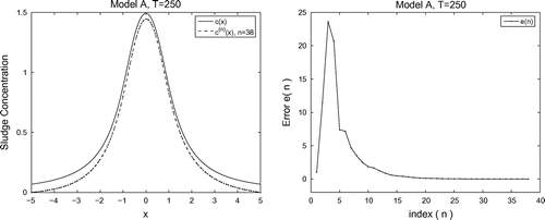
To analyze the convergence of the iteration algorithm (11) and (12) and the accuracy of the difference scheme (15), let us consider the following numerical test example.

Example 1

For the given data $\mathit{\nu }(t)=1+1/\sqrt{t+1}$, $D(x)=1$, $\mathit{\phi }(x)=exp(-{(x^2+1)}^2)$, ${\mathit{\alpha }}_1(t)=0$, ${\mathit{\alpha }}_2(t)=0$, the function $u(x,t)={(t+1)}^{-3/2}exp(-{(x^2+1)}^2/(t+1))$ is an exact (analytical) solution of the problem16 $$\begin{array}{c}\hfill \left\{\begin{array}{c}{u}_t={\left(D,(x),u_x\right)}_x-\mathit{\nu }(t){(c(x)u)}_x+f(x,t),(x,t)\in (-L,L)\times (0,T],\hfill \\ u(-L,t)={\mathit{\alpha }}_1(t),u(L,t)={\mathit{\alpha }}_2(t),t\in (0,T],\hfill \\ u(x,0)=\mathit{\phi }(x),x\in (-L,L),\hfill \\ {\int }_0^{T}u(x,t)dt=c(x),x\in (-L,L),\hfill \end{array}\right.\end{array}$$16 where $T>0$ denotes the final time and simulates the infinity. The source function $f(x,t)$ is obtained from the analytical solution $u(x,t)$ and input data $D(x),\mathit{\nu }(t),c(x)$ by using symbolic mathematics toolbox in MATLAB. The value of $T>0$ will be defined below. The length parameter $L>0$ is chosen large enough to simulate the initial model (1). Here this value is taken to be $L=5$. Calculating the integral in (1) over $(0,\infty )$ we found $c(x)=\sqrt{\mathit{\pi }}erf(x^2+1)/(x^2+1)$. Thus the pair $〈u(x,t),c(x)〉$ is exact (analytical) solution of the identification problem (9) and (10), corresponding to the Model A.

The iteration scheme (11) and (12) is applied for determination of the approximate numerical solution $y_i^j=y(x_i,t_j)$ of this problem. At each $n$th step of this iteration scheme the linear transport-diffusion problem (11) is solved by the difference scheme (15), and the integral in (12) is calculated by the trapezoidal rule. Results of computational experiments for various grid parameters $h_x,h_t>0$ are given in Table 1. The condition $\Vert c^{(n)}-c^{(n-1)}{\Vert }_{\infty }<{\mathit{\epsilon }}_c$, with ${\mathit{\epsilon }}_c=1.0\times {10}^{-3}$, is used as a stopping criterion in this iteration process. Optimal values of grid parameters are obtained to be $h_x=0.5$ (or $h_x=0.25$), $h_t=1.0$, as the values of sup-norm errors $\Vert u-u_h{\Vert }_{\infty }$, $\Vert c-c_h{\Vert }_{\infty }$ given in Table 1 show. Numerical solutions of the identification problem (16), corresponding to these values of grid parameters and to the final time values $T=250$ and $T=500$ are very close, as the sixth and seventh columns of the table show. This means that the value $T=250$ can be taken as optimal value of the final time $T>0$ in subsequent computational experiments.

For the value ${\mathit{\epsilon }}_c=1.0\times {10}^{-3}$, of the stopping parameter, the elapsed CPU time was about $20÷40$ sec. Here and below all computational experiments were done with computers PENTIUM(R) Dual Core processor, E5300, 2.6 GHz. The number of iterations is given in the last column of Table 1. Note that next decrease of the stopping parameter ${\mathit{\epsilon }}_c>0$ does not effect on the numerical values of the coefficient $c(x)$. Thus in combination with the difference scheme (15), the proposed iteration process has high accuracy, and its convergence is fast enough.

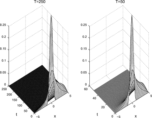
The behavior of the density function $u(x,t)$ for the optimal final time value $T=250$ and for the intermediate time value $T=50$ are given in the left and right upper Figure 2, respectively. The small compact support of the both functions $u(x,t)$ show that in the case of homogeneous boundary conditions the identification problem (1) can indeed be considered in the finite parabolic domain $(-L,L)\times (0,T]$, choosing an approximate $L>0$. The left below Figure 3 shows exact solution $c(x)$ (solid line )and the approximate solution $c^{(n)}(x)$ (dashed line) of identification problem (16). The errors $e(n):=\Vert c^{(n+1)}-c^{(n)}{\Vert }_{\infty }$ are plotted in the right below Figure 3. The optimal values of iterations were found $n=35÷40$ as the Figure 3 shows.

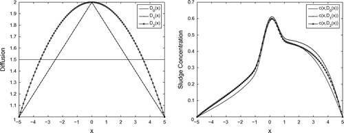
Next series of computational experiments is related to an influence of the variable diffusion coefficient $D(x)$ to the behavior of the sludge concentration $c(x)$ in the Model A. For this aim, the piecewise linear diffusion coefficient17 $$\begin{array}{c}\hfill D_1(x)=\left\{\begin{array}{cc}2+x/L,\hfill & x\in [-L,0);\hfill \\ 2-x/L,\hfill & x\in [0,L],\hfill \end{array}\right.\end{array}$$17 its average, i.e. the constant $D_0(x)=1.5$, and the function $D_2(x)=2-x^2/L^2$, obtained by ‘smoothing’ the piecewise linear diffusion coefficient $D_1(x)$, were assumed to be three different input data in the identification problem (16) (the left Figure 4). Other input functions and parameters in the identification problem (16) were taken to be as in Example 1. Numerical values of the sludge concentration functions $c(x;D_i)$ corresponding to the variable coefficients $D_i(x)$ are obtained to be close to the constant diffusion coefficient case. The results of computational experiments are given in the right Figure 4. The curves plotted in this figure show that an influence arising from the averaging/smoothing of the diffusion coefficient $D(x)$ can be neglected in the range of acceptable scales: ${max}_{[-L,L]}{D}_i(x)-{min}_{[-L,L]}{D}_i(x)=1$, $i=1,2$.

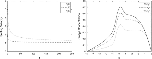
To find out an influence of the velocity function $\mathit{\nu }(t)$ to the behavior of the sludge concentration $c(x)$ in the Model A, the nonlinear identification problem (1) and (2) is analyzed for different settling velocity functions. For this aim the input data $f(x,t)\equiv 0$, $\mathit{\phi }(x)=exp(-{(x^2+1)}^2)$, ${\mathit{\alpha }}_1(t)=0$, ${\mathit{\alpha }}_2(t)=0$, $h_x=0.25$, $h_t=1.0$, $L=5$ and $T=250$, with the constant diffusion coefficient $D(x)\equiv 1$, are used in the computational experiments below. The behavior of the sludge concentration $c(x)$ in the settler is studied for the following settling velocity functions: ${\mathit{\nu }}^{(0)}(t)\equiv 1$, ${\mathit{\nu }}^{(1)}(t)=1+1/\sqrt{t+1}$ and ${\mathit{\nu }}^{(2)}(t)=1+5/\sqrt{t+1}$ (the left Figure 5). Note that ${\mathit{\nu }}^{(0)}(t)<{\mathit{\nu }}^{(1)}(t)<{\mathit{\nu }}^{(2)}(t)$, and the constant velocity function ${\mathit{\nu }}^{(0)}(t)$ can be treated as a limiting case of the time dependent velocity functions ${\mathit{\nu }}^{(k)}(t)=1+5/(k\sqrt{t+1})$, $k=1,2,3,...$, when $k\to \infty$. The computational results show that $n=22$ iterations are required for the value ${\mathit{\epsilon }}_c=1.0\times {10}^{-3}$ of the stopping parameter ${\mathit{\epsilon }}_c>0$. The obtained numerical results are plotted in Figure 4(b). This figure shows that the mapping $\mathit{\nu }(t)\mapsto c(x)$ is an antitone one. Specifically, ${\mathit{\nu }}^{(0)}(t)<{\mathit{\nu }}^{(1)}(t)<{\mathit{\nu }}^{(2)}(t)$ implies $c^{(0)}[{\mathit{\nu }}^{(0)}]>c^{(0)}[{\mathit{\nu }}^{(1)}]>c^{(0)}[{\mathit{\nu }}^{(2)}]$. This means that the sludge concentration decreases by increasing the settling velocity.

Table 1. Results of computational experiments for the Model A.

Final time ($T$)	$N$	$M$	$h_x$	$h_t$	$\frac{\Vert u-u_h{\Vert }_{\infty }}{{\Vert u\Vert }_{\infty }}$	$\frac{\Vert c-c_h{\Vert }_{\infty }}{{\Vert c\Vert }_{\infty }}$	Number of iterations
50	21	26	0.5	2.0	$6.29\times {10}^{-2}$	$1.38\times {10}^{-1}$	24
250	21	84	0.5	3.0	$\mathbf{5}.\mathbf{53}\times {\mathbf{10}}^{-\mathbf{2}}$	$\mathbf{8}.\mathbf{04}\times {\mathbf{10}}^{-\mathbf{2}}$	25
250	21	251	0.5	1.0	$5.57\times {10}^{-2}$	$8.24\times {10}^{-2}$	34
500	21	101	0.5	5.0	$7.74\times {10}^{-2}$	$2.1\times {10}^{-1}$	20
500	21	501	0.5	1.0	$\mathbf{5}.\mathbf{26}\times {\mathbf{10}}^{-\mathbf{2}}$	$\mathbf{6}.\mathbf{88}\times {\mathbf{10}}^{-\mathbf{2}}$	35
500	41	501	0.25	1.0	$2.27\times {10}^{-2}$	$4.65\times {10}^{-2}$	38

Figure 5. An influence of the settling velocity $\mathit{\nu }(t)$ to the sludge concentration $c(x)$.

4 Computational analysis of the Model B

The Model B can be formulated as the following identification problem: Find pair of functions $〈u(x,t),c(x)〉$ satisfying the following linear parabolic problem:18 $$\begin{array}{c}\hfill \left\{\begin{array}{c}{u}_t(x,t)={(D(x)u_x(x,t))}_x-{\mathit{\nu }}_0{(exp(-{\mathit{\alpha }}_{0}c(x))u(x,t))}_x,(x,t)\in {\mathrm{\Omega }}_T\hfill \\ u(x,0)=\mathit{\phi }(x),x\in (-L,L),\hfill \\ u(-L,t)=u(L,t)=0,t\in (0,T],\hfill \end{array}\right.\end{array}$$18 from the nonlocal additional condition19 $$\begin{array}{c}\hfill {\int }_0^{T}u(x,t)dt=c(x),x\in (-L,L).\end{array}$$19 When the sludge concentration function $c(x)$ is known, then the parabolic problem (18) defines the linear direct problem.

Applying the similar linearization (iteration) scheme, given for Model A above, to the identification problem (18) and (19) we obtain:20 $$\begin{array}{c}\hfill \left\{\begin{array}{c}{u}_t^{(n)}={(D(x)u_x^{(n)})}_x-{\mathit{\nu }}_0{(N(c^{(n-1)})u^{(n)})}_x,(x,t)\in {\mathrm{\Omega }}_T\hfill \\ u^{(n)}(x,0)=\mathit{\phi }(x),x\in (-L,L),\hfill & n=1,2,3,...\hfill \\ u^{(n)}(-L,t)=u^{(n)}(L,t)=0,t\in (0,T],\hfill \end{array}\right.\end{array}$$20 where21 $$\begin{array}{c}\hfill N(c^{(n-1)})(x):=exp\left(-,{\mathit{\alpha }}_0,c^{(n-1)},(x)\right)\end{array}$$21 is a nonlinear operator, and22 $$\begin{array}{c}\hfill c^{(n-1)}(x):={\int }_0^T{u}^{(n-1)}(x,t)dt,x\in (-L,L).\end{array}$$22 The function $u^{(n)}(x,t)$ represents an approximate solution of the identification problem (18) and (19). Assuming $w(x,t):=u^{(n)}(x,t)$, we conclude that the function $w(x,t)$ solves the linear parabolic problem (4) with the transport term ${\mathit{\nu }}_0{(\tilde{N}(x)w)}_x$, where $\tilde{N}(x):=N(c^{(n-1)})(x)$. Thus the finite-difference scheme (15) and Theorem 1 can be applied to the this model.

Theorem 3

Let $u^{(n)}(x,t)\in {\mathring{V}}^{1,0}({\mathrm{\Omega }}_t)$ be solution of the linearized parabolic problem (20) and (21). Assume that $c(x)\in C^1[-L,L]$ and conditions of Theorem 1 hold. Then,23 $$\begin{array}{c}\hfill \Vert u^{(n+1)}-u^{(n)}{\Vert }_{{\mathring{V}}^{1,0}({\mathrm{\Omega }}_t)}\le {\mathit{\alpha }}_0{C}_0\sqrt{2L}\mathcal{M}{e}^{\mathit{\lambda }t}{\Vert u^{(n)}-u^{(n-1)}\Vert }_{{\mathring{V}}^{1,0}({\mathrm{\Omega }}_t)},\forall t\in (0,T].\end{array}$$23

Proof

Applying estimation (7) for the case $Q(c(x),t):=e^{-{\mathit{\alpha }}_{0}c(x)}$, we have$$\begin{array}{c}\hfill \begin{array}{cc}\Vert u^{(n+1)}-u^{(n)}{\Vert }_{{\mathring{V}}^{1,0}({\mathrm{\Omega }}_t)}\hfill & \le \mathcal{M}{e}^{\mathit{\lambda }t}{sup}_{[-L,L]}|e^{-{\mathit{\alpha }}_0{c}^{(n)}(x)}-e^{-{\mathit{\alpha }}_0{c}^{(n-1)}(x)}|\hfill \\ \hfill & \le \mathcal{M}{e}^{\mathit{\lambda }t}{sup}_{[-L,L]}{\mathit{\alpha }}_0{e}^{-{\mathit{\alpha }}_{0}c(x)}|c^{(n)}(x)-c^{(n-1)}(x)|\hfill \\ \hfill & ={\mathit{\alpha }}_0{C}_0\mathcal{M}{e}^{\mathit{\lambda }t}{\Vert {\int }_0^T\left[u^{(n)},(x,t),-,u^{(n-1)},(x,t)\right]dt\Vert }_{L^2[-L,L]}.\hfill \end{array}\end{array}$$Estimating the right hand side integral as in the proof of Theorem 2 we get the required result. $\square$

For $t=T$, estimate (23) has the form:$$\begin{array}{c}\hfill \Vert u^{(n+1)}-u^{(n)}{\Vert }_{{\mathring{V}}^{1,0}({\mathrm{\Omega }}_T)}\le {\mathit{\alpha }}_0{C}_0\sqrt{2L}\mathcal{M}{e}^{\mathit{\lambda }T}{\Vert u^{(n)}-u^{(n-1)}\Vert }_{{\mathring{V}}^{1,0}({\mathrm{\Omega }}_T)}.\end{array}$$Requiring$$\begin{array}{c}\hfill {\mathit{\alpha }}_0{C}_0\sqrt{2L}\mathcal{M}{e}^{\mathit{\lambda }T}<1\end{array}$$we conclude following result if the conditions of convergence in Theorem 3 hold.

Conclusion 2.    Let conditions of Theorem 3 hold. Assume that the arbitrary parameter $\mathit{\epsilon }>0$ in $\mathcal{M}$ is defined so that the condition$$\begin{array}{c}\hfill \mathit{\lambda }<-log({\mathit{\alpha }}_0{C}_0\sqrt{2L}\mathcal{M})/T.\end{array}$$holds. Then the iteration scheme defined by (20) and (21) converges in the norm of the space ${\mathring{V}}^{1,0}({\mathrm{\Omega }}_T)$.

Table 2. Results of computational experiments for the Model B.

Final time ($T$)	$N$	$M$	$h_x$	$h_t$	$\frac{\Vert u-u_h{\Vert }_{\infty }}{{\Vert u\Vert }_{\infty }}$	$\frac{\Vert c-c_h{\Vert }_{\infty }}{{\Vert c\Vert }_{\infty }}$	Number of iterations
50	21	26	0.5	2.0	$\mathbf{4}.\mathbf{40}\times {\mathbf{10}}^{-\mathbf{2}}$	$\mathbf{1}.\mathbf{78}\times {\mathbf{10}}^{-\mathbf{1}}$	5
50	41	51	0.25	1.0	$1.92\times {10}^{-2}$	$1.90\times {10}^{-1}$	6
250	21	251	0.5	1.0	$2.86\times {10}^{-2}$	$8.58\times {10}^{-2}$	6
250	41	251	0.25	1.0	$\mathbf{1}.\mathbf{90}\times {\mathbf{10}}^{-\mathbf{2}}$	$\mathbf{8}.\mathbf{53}\times {\mathbf{10}}^{-\mathbf{2}}$	6
500	21	101	0.5	5.0	$5.41\times {10}^{-2}$	$2.74\times {10}^{-1}$	5
500	21	501	0.5	1.0	$\mathbf{2}.\mathbf{88}\times {\mathbf{10}}^{-\mathbf{2}}$	$\mathbf{6}.\mathbf{44}\times {\mathbf{10}}^{-\mathbf{2}}$	6

Since the accuracy of the solution to the considered identification problem strictly depends on the accuracy of the numerical solution of the corresponding to the linear problem, one needs first to derive an optimal mesh for numerical solution of linearized problem (20) and (21).

Figure 6. The ‘square wave’ initial density function $u(x,0)=\mathit{\phi }(x)$ (the left figure) and the corresponding solution $c^{(n)}(x)$ (the right figure) of the identification problem (17) in the Model B.

Figure 7. The behaviour of the density function $u(x,t)$ for Model B.

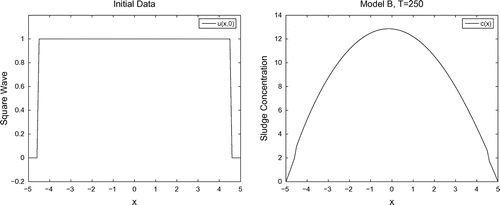
Figure 8. Behavior of the sludge concentration $c(x)$ for various values of the maximum settling velocity ${\mathit{\nu }}_0>0$ and the model parameter ${\mathit{\alpha }}_0>0$, given in [17], and for different initial data.

Example 2

For the given data ${\mathit{\alpha }}_0=0.5$, ${\mathit{\nu }}_0=1$, $D(x)=1+x^2$, $\mathit{\phi }(x)=exp(-{(x^2+1)}^2)$, the function $u(x,t)={(t+1)}^{-3/2}exp(-{(x^2+1)}^2/(t+1))$ is an exact (analytical) solution of the problem24 $$\begin{array}{c}\hfill \left\{\begin{array}{c}{u}_t={\left(D,(x),u_x\right)}_x-{\mathit{\nu }}_0{(exp(-{\mathit{\alpha }}_{0}c(x))u)}_x+f(x,t),(x,t)\in (-L,L)\times (0,T],\hfill \\ u(-L,t)=0,u(L,t)=0,t\in (0,T],\hfill \\ u(x,0)=\mathit{\phi }(x),x\in (-L,L),\hfill \\ {\int }_0^{T}u(x,t)dt=c(x),x\in (-L,L).\hfill \end{array}\right.\end{array}$$24 To simulate infinity in the initial model (1), here the length parameter $L>0$ is again taken to be $L=5$ in practice. The source function $f(x,t)$ is obtained from the analytical solution $u(x,t)$ and input data $D(x),c(x)$ by using symbolic mathematics toolbox in MATLAB. Calculating the integral in (21) over $(0,\infty )$ we obtain $c(x)=\sqrt{\mathit{\pi }}erf(x^2+1)/(x^2+1)$. Thus the pair $〈u(x,t),c(x)〉$ is exact (analytical) solution of the identification problem (21), corresponding to the Model B.

Results of computational experiments are presented in Table 2. As in the case of the Model A, the optimal values of grid parameters are obtained to be $h_x=0.5$, $h_t=1.0$. Further, the numerical results corresponding to the final time values $T=250$ and $T=500$ are obtained to be very close as seen easily from the fifth column of Table 2. Hence the value $T=250$ can be taken as optimal value of the final time $T>0$ for the Model B, also. $\square$

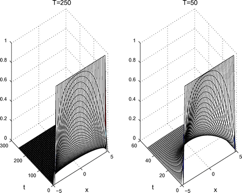
Now, we consider identification problem (18) and (19). The behaviour of the density function $u(x,t)$ within the Model B is analyzed for ‘square wave’ form which is initial data $u(x,0)=\mathit{\phi }(x)$, given in the left Figure 6. The right Figure 6 illustrates the corresponding solution of the identification problem (18) and (19), i.e. the sludge concentration function $c(x)$. For the optimal final time value $T=250$ and for the intermediate time value $T=50$ in problem (17), the behaviour of the density of sludge concentration function $u(x,t)$ are presented in left and right Figure 7, respectively. In the both cases the function $u(x,t)$ rapidly tends to zero as the time variable $t>0$ increases. The small compact support of the both functions $u(x,t)$ show that in the case of homogeneous Dirichlet boundary conditions the identification problem (18) and (19) can indeed be considered in the finite parabolic domain $(-L,L)\times (0,T]$.

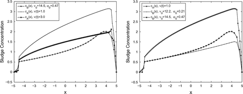
To study an influence of the initial density $u(x,0)=\mathit{\phi }(x)$ to the further behavior of the sludge concentration, series of computational experiments are realized for two different input data: ${\mathit{\phi }}_1(x)=exp(-{(x^2+1)}^2)$, and ${\mathit{\phi }}_2(x)$ is the ‘square wave’ function given in the left Figure 6. The left and right Figure 8 illustrates the corresponding sludge concentration functions. The left Figure 8 corresponds to the input data ${\mathit{\phi }}_1(x)$, and shows the behavior of the sludge concentration $c(x)$ for various values of the maximum settling velocity ${\mathit{\nu }}_0>0$ and the model parameter ${\mathit{\alpha }}_0>0$, given in [17]. Bold faced solid line here corresponds to the gravity induced sludge velocity model25 $$\begin{array}{c}\hfill v(c)=14.5e^{-0.47c}\end{array}$$25 The both figures show that if the relative measurement errors$$\begin{array}{c}\hfill {\mathit{\gamma }}_{{\mathit{\nu }}_0}:=\frac{|{\mathit{\nu }}_0-\widetilde{{\mathit{\nu }}_0}|}{{\mathit{\nu }}_0}\times 100\%,{\mathit{\gamma }}_{{\mathit{\alpha }}_0}:=\frac{|{\mathit{\alpha }}_0-\widetilde{{\mathit{\alpha }}_0}|}{{\mathit{\alpha }}_0}\times 100\%\end{array}$$are of about $6÷7\%$, then the behavior of the sludge concentration $c(x)$ is the same as in the gravity induced sludge velocity model. Hence an influence of the initial density $u(x,0)=\mathit{\phi }(x)$ to the further behavior of the sludge concentration is more essential than the influence of the model parameters ${\mathit{\nu }}_0>0$ and ${\mathit{\alpha }}_0>0$, as the computational experiments show.

5 Comparative analysis of the models

To compare the behavior of the sludge concentration $c(x)$ within the Model A and Model B, first we consider the ‘square wave’ initial density case for both models (with the input data $D(x)\equiv 1$, $h_x=0.25$, $h_t=1.0$, $T=250$). The left Figure 9 illustrates results of computational experiments for the cases when ${\mathit{\nu }}^{(1)}(t)=1.0$ and ${\mathit{\nu }}^{(2)}(t)=3.0$ in the Model A, and ${\mathit{\nu }}_0=14.5$, ${\mathit{\alpha }}_0=0.47$ in the Model B (the gravity induced sludge velocity model, given by (22)). Here and below the sludge concentration function $c^{(k)}(x)$ corresponds to the velocity parameter ${\mathit{\nu }}_0^{(k)}$, in the Model A, and to the pairs $〈{\mathit{\nu }}_0^{(1)},{\mathit{\alpha }}_0^{(1)}〉$, in the Model B. The right Figure 9 illustrates the behaviour of the sludge concentration computational within the Model B, when $〈{\mathit{\nu }}_0^{(1)},{\mathit{\alpha }}_0^{(1)}〉$$=〈12.2,0.21〉$ and $〈{\mathit{\nu }}_0^{(2)},{\mathit{\alpha }}_0^{(2)}〉$$=〈14.5,0.47〉$, and within the Model A, when $\mathit{\nu }(t)=1.0$. Comparison of the results presented in both figures show that the behaviour of the sludge concentration function $c(x)$ is almost linear within the Model A, when the velocity function $\mathit{\nu }(t)$ is a constant. At the same time, this behaviour is nonlinear within the Model B for each input data $〈{\mathit{\nu }}_0,{\mathit{\alpha }}_0〉$. Note that the rapid decay of the function $c(x)$ in the neighborhood of the endpoints $x=\pm L$ is due to the homogeneous boundary conditions ($u(-L,t)=u(L,t)=0$).

Figure 9. Comparative analysis of the models: The behaviour of the sludge concentration function $c(x)$.

Figure 10. Comparative analysis of the models: Noise free($c_A,c_B$) and noisy ($c_A^{\mathit{\gamma }},c_B^{\mathit{\gamma }}$).

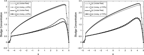
To analyze the sensitivity of the sludge concentration function $c(x)$ with respect to the input data $〈{\mathit{\nu }}_0,{\mathit{\alpha }}_0〉$ series of computational experiments were performed for the both considered models. The left and right Figure 10 shows noise free ($c_A(x)$, $c_B(x)$) and noisy ($c_A^{\mathit{\gamma }}(x)$, $c_B^{\mathit{\gamma }}(x)$) numerical solutions corresponding to the Model A and Model B. The noise factors $\mathit{\gamma }$ in the noisy parameters ${\mathit{\nu }}_{\mathit{\gamma }}=\mathit{\nu }\pm \mathit{\gamma }·\mathit{\nu }$ and ${\mathit{\alpha }}_{\mathit{\gamma }}=\mathit{\alpha }\pm \mathit{\gamma }·\mathit{\alpha }$ are assumed to be $\mathit{\gamma }=5\%$ (left figure) and $\mathit{\gamma }=10\%$ (right figure). The noise free input data $〈\mathit{\nu },\mathit{\alpha }〉$ in the computational experiments are assumed to be as $\mathit{\nu }(t)=1.0$ in the Model A, and ${\mathit{\nu }}_0=14.5,{\mathit{\alpha }}_0=0.47$ in the Model B. The relative errors defined to be as$$\begin{array}{c}\hfill {\mathit{\epsilon }}^{(A)}(\mathit{\gamma })=\frac{\Vert c_A-c_A^{\mathit{\gamma }}{\Vert }_{\infty }}{\Vert c_A{\Vert }_{\infty }}\times 100\%,{\mathit{\epsilon }}^{(B)}(\mathit{\gamma })=\frac{\Vert c_B-c_B^{\mathit{\gamma }}{\Vert }_{\infty }}{\Vert c_B{\Vert }_{\infty }}\times 100\%\end{array}$$are obtained as follows:$$\begin{array}{c}\hfill \begin{array}{c}{\mathit{\epsilon }}^{(A)}(\mathit{\gamma }=5\%)=2.23\%,{\mathit{\epsilon }}^{(A)}(\mathit{\gamma }=10\%)=4.45\%,\\ {\mathit{\epsilon }}^{(B)}(\mathit{\gamma }=5\%)=17.4\%,{\mathit{\epsilon }}^{(B)}(\mathit{\gamma }=10\%)=3.87\%.\end{array}\end{array}$$These results show that the noise levels $\mathit{\gamma }=5\%$ and $\mathit{\gamma }=10\%$ in the measured input data $〈{\mathit{\nu }}_0,{\mathit{\alpha }}_0〉$ are acceptable within the considered models.

6 Conclusions

We have discussed two age dependent transport-diffusion settler models. Both model leads to a nonlinear identification problem with additional (nonlocal) integral conditions. We proposed an iteration (linearization) algorithm for solving this identification problem. This iteration scheme leads both models to the basic problem, which mathematical analysis is given in detail. These results are then applied each model to prove convergence of iterations. An effective numerical algorithm for computational simulation of these models is proposed. The algorithm is tested for the both models. Computational simulation permits one to estimate an influence of the model parameters ${\mathit{\nu }}_0>0$ and ${\mathit{\alpha }}_0>0$ the behaviour of the sludge concentration $c(x)$.

Acknowledgments

The author gratefully thank the anonymous referees for valuable suggestions which improved the manuscript. The author also would like to thank Prof. Dr Alemdar Hasanoglu (Hasanov) for his valuable comments and suggestions leading to a better presentation of this article.

Notes

1 The work has been supported by the Scientific and Technological Research Council of Turkey (TUBITAK) through the research project [grant number 108T332].

References

- David R, Vasel J-L, Vande Wouwer A. Settler dynamic modeling and MATLAB simulation of the activated sludge process. Chem. Eng. J. 2009;146:174–183.
- Ossenbrungen P, McIntire S. Using shock wave theory to predict clarifier performance. In: Yokohama, Kyoto,editors. Proceedings of the 5th IAWPRC Workshop. Japan: Plenum Press; 1990. p. 479–486
- Laikari S. Simulation of the sludge blanket of a vertical clarifier in activated sludge process. Water Sci. Tech. 1989;21:621–629.
- Takacs I, Party G, Nolasco D. A dynamic model of the clarification-thickening process. Water Res. 1991;25:1263–1271.
- Chancelier JP, de Lara MC, Pacard F. Analysis of a conservation PDE with discontinuous flux: a model of settler. SIAM J. Appl. Math. 1994;54:954–995.
- Chancelier JP, de Lara MC, Joannis C, Pacard F. New insights in dynamic modeling of a secondary settler - I. Flux theory and steady state analysis, Water Res. 1997;31:1847–1856.
- Chancelier JP, de Lara MC, Joannis C, Pacard F. New insights in dynamic modeling of a secondary settler - II. Dynamic analysis, Water Res. 1997;31:1857–1866.
- Hasanov A, Mueller J. A numerical method for backward parabolic problems with non-selfadjoint elliptic operator. Appl. Numer. Math. 2001;37:55–78.
- Chancelier JP, de Lara MC, Pacard F. Existence of a solution in an age-dependent transport-diffusion PDE: a model of settler. Math. Models Meth. Appl. Sci. 1995;5:267–278.
- Pektas B. Modeling and computer simulation of the identification problem related to the sludge concentration in a settler. Math. Comput. Model. 2009;49:843–855.
- Lenhart S. Optimal control of a convective-diffusive fluid problem. Math. Models Meth. Appl. Sci. 1995;5:225–237.
- Vesilind AP. Design of prototype thickeners from batch settling tests. Water Sewage Works. 1968;115:302–307.
- Vanderhasselt A, Vanrolleghem PA. Estimation of sludge sedimentation parameters from single bath settling curves. Water Res. 2000;34:395–406.
- Vitasovic Z. Continuous settler operation: a dynamic model. In: Party GG, Chapman D, editors. Dynamic modeling and expert systems in wastewater engineering. Chelsea: Lewis Publishers; 1989. p. 59–81.
- Hasanov A, Pektas B, Kadiroglu U. An analysis of nonlinear ion transport problem including arbitrary valences of oxidized and reduced species. J. Math. Chem. 2010;47:1248–1262.
- Munavalli GR, Kumar MSM. Water quality parameter estimation in a distribution system under dynamic state. Water Res. 2005;39:4287–4298.
- Smolianski A, Shipilova O, Haario H. A fast high-resolution algorithm for linear convection problems: particle transport method. Int. J. Numer. Meth. Eng. 2007;70:655–684.
- Vairaktaris E, Vardoulakis I, Papamichos E, Dougalis V. Subsidence diffusion-convection. II. The inverse problem. Comput. Meth. Appl. Mech. Eng. 2004;193:2761–2770.
- Ladyzhenskaya OA. Boundary value problems in mathematical physics. New York (NY): Springer Verlag; 1985.
- Samarskii AA. The theory of difference schemes. New York (NY): Marcel Dekker; 2001.