Generalized finite difference method for solving two-dimensional inverse Cauchy problems

Abstract

In this paper, a meshless numerical scheme is adopted for solving two-dimensional inverse Cauchy problems which are governed by second-order linear partial differential equations. In Cauchy problems, over-specified boundary conditions are imposed on portions of the boundary while on parts of boundary no boundary conditions are imposed. The application of conventional numerical methods to Cauchy problems yields highly ill-conditioned matrices. Hence, small noise added in the boundary conditions will tremendously enlarge the computational errors. The generalized finite difference method (GFDM), which is a newly developed domain-type meshless method, is adopted to solve in a stable manner the two-dimensional Cauchy problems. The GFDM can overcome time-consuming mesh generation and numerical quadrature. Besides, Cauchy problems can be solved stably and accurately by the GFDM. We present three numerical examples to validate the accuracy and the simplicity of the meshless scheme. In addition, different levels of noise are added into the boundary conditions to verify the stability of the proposed method.

Keywords:

• meshless numerical scheme
• Cauchy problems
• generalized finite difference method
• noise
• stability

Nomenclature

Table

$a_1=a_1(x,y)$	given coefficient functions
$a_2=a_2(x,y)$	given coefficient functions
$a_3=a_3(x,y)$	given coefficient functions
$a_4=a_4(x,y)$	given coefficient functions
$a_5=a_5(x,y)$	given coefficient functions
$a_6=a_6(x,y)$	given coefficient functions
$a_7=a_7(x,y)$	given coefficient functions
$d{m}_i$	supporting radius of weighting function for the ith node
$f(x,y)$	given boundary condition
$g(x,y)$	given boundary condition
$h(x,y)$	given boundary condition
$l(x,y)$	given boundary condition
$\overrightarrow{n}=(n_x,n_y)$	unit outward normal vector
$N$	number of total nodes
$n_b$	number of boundary nodes
$n_i$	number of interior nodes
$n_s$	number of nodes in a star
rand	random number
$s$	percentage of added noise
$u(x,y)$	(unknown) solution
$u_n(x,y)$	normal derivative of the (unknown) solution
$w(d_{ij})$	weighting function
${\{w{x}_j^i\}}_{j=0}^{n_s}$	weighting coefficients
${\{w{y}_j^i\}}_{j=0}^{n_s}$	weighting coefficients
${\{wx{x}_j^i\}}_{j=0}^{n_s}$	weighting coefficients
${\{wy{y}_j^i\}}_{j=0}^{n_s}$	weighting coefficients
${\{wx{y}_j^i\}}_{j=0}^{n_s}$	weighting coefficients
$(x_i,y_i)$	coordinates of the ith node
$(x_j^i,y_j^i)$	coordinates of the other nodes in the ith star
${\mathrm{\Gamma }}_d$	boundary portions with Dirichlet boundary condition
${\mathrm{\Gamma }}_n$	boundary portions with Neumann boundary condition
${\mathrm{\Gamma }}_o$	boundary portions with over-specified boundary condition
$\mathrm{\Omega }$	computational domain
$\mathit{\gamma }$	boundary portions with no boundary condition

1. Introduction

There are many inverse problems that appear in realistic engineering applications.[1–7] In some of these portions, boundary conditions are missing,[1–3] and in some, boundary spatial positions are missing.[4–7] For example, Fu et al. [1] adopted the boundary particle method to solve the Cauchy inhomogeneous potential problems, while Lesnic et al. [3] used the boundary element method and an iteration procedure to resolve inverse problems governed by two-dimensional biharmonic equations. Fan and Chan [4] applied the modified collocation Trefftz method (MCTM) to identify portions of boundary spatial positions in heat conduction problems, while Karageorghis and Lesnic [6] numerically detected inner cavities by using the method of fundamental solutions (MFS). When numerical simulation is considered to solve the inverse problems, the resulting ill-conditioned matrices will enlarge the computational errors. Thus, many numerical schemes have been proposed in the past to stably analyse inverse problems. In this paper, we will use a promising meshless numerical method for the stable and accurate solution of inverse Cauchy problems.

In the past decades, many numerical methods have been proposed for the solution of Cauchy problems.[8–11] For instance, Liu and Atluri [9] solved Cauchy problems, governed by the Laplace equation, by using the MCTM and a conditioner. The multiple-scale characteristic lengths were used to form a matrix conditioner to reduce the condition number of the coefficient matrix. Young et al. [11] numerically investigated the relations between the condition number and the positions of source points of the MFS for inverse problems governed by the Laplace equation. They could retrieve the optimal solution by tracing the residual norms of the system of linear algebraic equations. From the above-mentioned numerical schemes, it can be deduced that it is nontrivial to develop a stable and simple numerical scheme to solve Cauchy problems.

In addition to mesh-based numerical methods, there are many promising meshless methods proposed and developed in the past few decades, such as the MFS,[11,12] the MCTM,[13–15] the method of approximate particular solutions,[16,17] the local radial basis function collocation method (LRBFCM),[18–24] the diffuse approximation method (DAM),[25,26] and the generalized finite difference method (GFDM),[27–31]. Among them, the MFS and the MCTM are the two most popular boundary-type meshless methods. By using only boundary points, they can directly solve both direct and inverse problems without mesh generation and numerical quadrature. Although the implementations of the MFS and the MCTM are very easy and simple, they are only useful for solving homogeneous and linear partial differential equations with known fundamental solutions or T-complete functions. On the other hand, the LRBFCM and the GFDM are two popular domain-type meshless methods. To solve boundary value problems by these two methods, both boundary and interior nodes are needed. Although they require more nodes than boundary-type meshless methods, they can be used to resolve inhomogeneous partial differential equations without any fundamental solution or any set of T-complete functions. In addition, the concepts of local domain in the LRBFCM and the star in the GFDM yield a sparse matrix system in contrast to a fully populated matrix in the MFS and the MCTM. Therefore, the LRBFCM and the GFDM have great potential for tackling realistic engineering applications.

Kosec and Sarler [19] analysed Darcy’s flow by using the LRBFCM, while Fan et al. [20] adopted the LRBFCM to solve double-diffusive natural convection in porous media. Urena et al. [30] adopted the GFDM to analyse fourth-order partial differential equations, which are used to describe the plate-bending problems; in the meantime, Chan et al. [31] used the GFDM and the fictitious time integration method to solve nonlinear obstacle problems. Both of the GFDM and the LRBFCM have the same merits and great potential for dealing with engineering problems. There is a free parameter in the LRBFCM, which has great influence on the accuracy of the results. Recently, some numerical techniques have been proposed to determine this free parameter and the optimal placements of the centres in the radial basis function (RBF)-related meshless methods.[32–34] Similarly, the GFDM also has free parameters, such as weighting functions and number of nodes in a star. By properly choosing these parameters, the GFDM can be directly extended to practical problems without known analytical solutions.[31]

In addition, the DAM was proposed by Sadat and Prax in 1996.[25] In their study, by utilizing the Taylor series and the weighted least-squares method, the derivatives of unknown variables are expressed as linear combinations of function values of neighbouring nodes. The numerical procedures of the DAM [25,26] are very similar with those in the GFDM.[27–31] Therefore, it is reasonable to say that the basic idea of the DAM (and the GFDM) was proposed by Sadat and Prax in 1996 [25] and the explicit formulas of the GFDM were provided by Benito et al. in 2001 [27] by using the Cholesky method. In this paper, the GFDM is used for stably solving two-dimensional Cauchy problems governed by second-order linear partial differential equations. To the best of the authors’ knowledge, this is the first time the GFDM is applied for solving inverse Cauchy problems governed by second-order partial differential equations.

For every node, a circular star will be formed and the derivatives at the centre node will be expressed by linear summations of approximate values of the neighbouring nodes. To enforce the satisfaction of the governing equation at interior nodes and the boundary conditions at boundary nodes, a system of linear algebraic equations is formed. The solution and its derivatives can be found by solving the final system. The description of the Cauchy problem and the numerical procedure of the GFDM will be given after the motivation of this study is provided in the Introduction. There are three numerical examples in Section 4. The comparisons of numerical solutions with analytical solutions show the stability and the simplicity of the numerical scheme. Finally, a discussion and some conclusions are provided in the last section.

2. Inverse Cauchy problem

Two-dimensional inverse Cauchy problems governed by second-order linear partial differential equations are considered. In a Cauchy problem, an over-specified boundary condition is imposed on a part of boundary while on another part of boundary no boundary condition is imposed. The governing equation and the boundary conditions are described by the following equations:(1) $$a_1\frac{{\mathit{\partial }}^{2}u}{\mathit{\partial }{x}^2}+a_2\frac{{\mathit{\partial }}^{2}u}{\mathit{\partial }x\mathit{\partial }y}+a_3\frac{{\mathit{\partial }}^{2}u}{\mathit{\partial }{y}^2}+a_4\frac{\mathit{\partial }u}{\mathit{\partial }x}+a_5\frac{\mathit{\partial }u}{\mathit{\partial }y}+a_{6}u=a_7,(x,y)\in \mathrm{\Omega },$$(1) (2) $$u=f(x,y),(x,y)\in {\mathrm{\Gamma }}_o,$$(2) (3) $$u_n=(\mathrm{\nabla }u)·\overrightarrow{n}=g(x,y),(x,y)\in {\mathrm{\Gamma }}_o,$$(3) (4) $$u=h(x,y),(x,y)\in {\mathrm{\Gamma }}_d,$$(4) (5) $$u_n=(\mathrm{\nabla }u)·\overrightarrow{n}=l(x,y),(x,y)\in {\mathrm{\Gamma }}_n,$$(5)

where $u(x,y)$ and $u_n(x,y)$ are the (unknown) solution and the normal derivative of the (unknown) solution. Moreover, $a_1=a_1(x,y)$, $a_2=a_2(x,y)$, $a_3=a_3(x,y)$, $a_4=a_4(x,y)$, $a_5=a_5(x,y)$, $a_6=a_6(x,y)$ and $a_7=a_7(x,y)$ are given coefficient functions, as well as $f(x,y)$, $g(x,y)$, $h(x,y)$ and $l(x,y)$ are given boundary conditions. Also, $\mathrm{\Omega }$ is the computational domain and $\mathit{\partial }\mathrm{\Omega }={\mathrm{\Gamma }}_o\cup {\mathrm{\Gamma }}_d\cup {\mathrm{\Gamma }}_n\cup \mathit{\gamma }$ is the boundary of the computational domain. ${\mathrm{\Gamma }}_o$, ${\mathrm{\Gamma }}_d$, ${\mathrm{\Gamma }}_n$ and $\mathit{\gamma }$ denote the boundary portions with the over-specified boundary condition, the Dirichlet boundary condition, the Neumann boundary condition and no boundary condition, respectively. The vector $\overrightarrow{n}=(n_x,n_y)$ is the unit outward normal vector.

The above governing equation and boundary conditions will form the Cauchy problem to which the GFDM will be applied. The description of the GFDM for solving the Cauchy problem will be given in the following section.

3. Generalized finite difference method

In order to solve Cauchy problems in a stable way, we adopted the GFDM to discretize the governing equation and the boundary conditions. The basic idea of the GFDM originates from the moving least squares method to approximate the derivatives at every node in a computational domain by linear summation of nodal values.

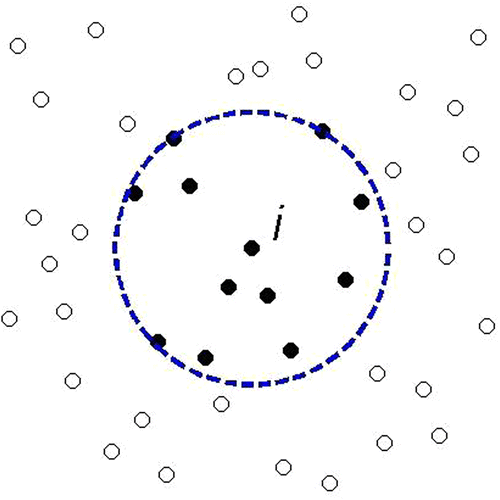
For a given ith node at the centre of the star, the $n_s$ nearest nodes around the ith node will be found. The ith node and the $n_s$ nearest nodes are used to form a star, which is shown in Figure 1. The largest distance between the ith node and the $n_s$ nearest nodes is denoted by $R_i$ and later we will use this distance to determine supporting radius of weighting function. In previous papers,[27,28] different choices for the shapes of the star are given. For the sake of simplicity, a circular star is used in this paper. From previous study,[27,28] it is clear that if more nodes are included in the star, the accuracy of the numerical results improved and, at the same time, the computational cost rose. Therefore, there will be an optimal choice for $n_s$ depending on the required accuracy and the available computer power. Moreover, from our experience,[31] accurate numerical results can be obtained when $n_s$ is larger than 10 for practical computation. Therefore, in the numerical experiments in this paper, the number $n_s$ is larger than 10.

Figure 1. Schematic diagram for the circular shape of the star.

Once the star for the ith node is formed, Taylor series is used to expand the function inside the star and a new functional, $B(u)$, will be defined. Let $u_i$ be the function value at the central node of the star with coordinates $(x_i,y_i)$ and $u_j^i$ ($j=1,2,3,\dots ,n_s$) denote the values at the other nodes inside the star with coordinates $(x_j^i,y_j^i)$. Defining a functional as [27–31]:(6) $$B(u)=\sum _{j=1}^{n_s}{\left[\left(u_i-u_j^i+h_{ij}\frac{\mathit{\partial }{u}_i}{\mathit{\partial }x}+k_{ij}\frac{\mathit{\partial }{u}_i}{\mathit{\partial }y}+\frac{1}{2}\left(h_{ij}^2\frac{{\mathit{\partial }}^2{u}_i}{\mathit{\partial }{x}^2}+k_{ij}^2\frac{{\mathit{\partial }}^2{u}_i}{\mathit{\partial }{y}^2}+2h_{ij}{k}_{ij}\frac{{\mathit{\partial }}^2{u}_i}{\mathit{\partial }x\mathit{\partial }y}\right)\right)w\left(h_{ij},k_{ij}\right)\right]}^2,$$(6)

where $j$ is the local index in the star. $h_{ij}=x_i-x_j^i$ and $k_{ij}=y_i-y_j^i$ are the distances between the ith node and the jth node along the x and y directions and $w(h_{ij},k_{ij})$ is the weighting function at $(x_j^i,y_j^i)$. There are many choices for the weighting functions,[27–31] such as potential function, cubic spline and quartic spline. The acceptable results can be acquired by adopting any of the above-mentioned weighting functions. Therefore, the quartic spline is adopted as the weighting function in this study:(7) $$w\left(d_{ij}\right)=\left\{\begin{array}{c}1-6{\left(\frac{d_{ij}}{d{m}_i}\right)}^2+8{\left(\frac{d_{ij}}{d{m}_i}\right)}^3-3{\left(\frac{d_{ij}}{d{m}_i}\right)}^4,d_{ij}⩽d{m}_i\hfill \\ 0,d_{ij}>d{m}_i\hfill \end{array}\right.,$$(7)

where $d_{ij}$ denotes the distance between nodes $\left(x_i,y_i\right)$ and $\left(x_j^i,y_j^i\right)$. $d{m}_i$ is the supporting radius of the weighting function, which can be determined arbitrarily, and will influence the stability and the accuracy of simulation. In this study, we examined the influence of the supporting radius on the numerical accuracy by numerical experiments.

Since only the distance between two nodes is used in Equation (7), the weighting function is one kind of RBFs. The weighting function is used to indicate the importance of the approximations at different nodes by Taylor series, which means that the approximation is more important if the node is closer to the centre of the star. Besides, the solution expression in the GFDM is based on Taylor series in contrast to the series expansion by RBFs in RBFs-based meshless methods,[18–24,32–34] so the GFDM is not one kind of the RBFs-based meshless methods.

To minimize the above functional with respect to ${\mathbf{D}}_{\mathbf{u}}={\left\{\begin{array}{ccccc}\frac{\mathit{\partial }{u}_i}{\mathit{\partial }x}& \frac{\mathit{\partial }{u}_i}{\mathit{\partial }y}& \frac{{\mathit{\partial }}^2{u}_i}{\mathit{\partial }{x}^2}& \frac{{\mathit{\partial }}^2{u}_i}{\mathit{\partial }{y}^2}& \frac{{\mathit{\partial }}^2{u}_i}{\mathit{\partial }x\mathit{\partial }y}\end{array}\right\}}^T$ yields a linear equation system:(8) $$\mathbf{A}{\mathbf{D}}_{\mathbf{u}}=\mathbf{b},$$(8)

where(9) $$\mathbf{A}=\left\{\begin{array}{ccccc}\sum _{j=1}^{n_s}{h}_{ij}^2{w}^2& \sum _{j=1}^{n_s}{h}_{ij}{k}_{ij}{w}^2& \sum _{j=1}^{n_s}\frac{h_{ij}^3}{2}{w}^2& \sum _{j=1}^{n_s}\frac{h_{ij}{k}_{ij}^2}{2}{w}^2& \sum _{j=1}^{n_s}{h}_{ij}^2{k}_{ij}{w}^2\\ & \sum _{j=1}^{n_s}{k}_{ij}^2{w}^2& \sum _{j=1}^{n_s}\frac{h_{ij}^2{k}_{ij}}{2}{w}^2& \sum _{j=1}^{n_s}\frac{k_{ij}^3}{2}{w}^2& \sum _{j=1}^{n_s}{h}_{ij}{k}_{ij}^2{w}^2\\ & & \sum _{j=1}^{n_s}\frac{h_{ij}^4}{4}{w}^2& \sum _{j=1}^{n_s}\frac{h_{ij}^2{k}_{ij}^2}{4}{w}^2& \sum _{j=1}^{n_s}\frac{h_{ij}^3{k}_{ij}}{2}{w}^2\\ & SYM& & \sum _{j=1}^{n_s}\frac{k_{ij}^4}{4}{w}^2& \sum _{j=1}^{n_s}\frac{h_{ij}{k}_{ij}^3}{2}{w}^2\\ & & & & \sum _{j=1}^{n_s}{h}_{ij}^2{k}_{ij}^2{w}^2\end{array}\right\},$$(9)

and(10) $$\mathbf{b}=\left\{\begin{array}{c}\sum _{j=1}^{n_s}\left(-u_i+u_j^i\right)h_{ij}{w}^2\\ \sum _{j=1}^{n_s}\left(-u_i+u_j^i\right)k_{ij}{w}^2\\ \sum _{j=1}^{n_s}\left(-u_i+u_j^i\right)\frac{h_{ij}^2}{2}{w}^2\\ \sum _{j=1}^{n_s}\left(-u_i+u_j^i\right)\frac{k_{ij}^2}{2}{w}^2\\ \sum _{j=1}^{n_s}\left(-u_i+u_j^i\right)h_{ij}{k}_{ij}{w}^2\end{array}\right\}.$$(10)

The coefficient matrix $\mathbf{A}$ is clearly symmetric. The explicit expressions for vector ${\mathbf{D}}_{\mathbf{u}}$ [27–31] depend on the number of nodes in the star, the spatial positions of the nodes and the weighting function. To decompose the vector $\mathbf{b}$, the vector is re-written as follows:(11) $$\mathbf{b}=\mathbf{BQ},$$(11)

where $\mathbf{Q}={[\begin{array}{cccccc}{u}_i& u_1^i& u_2^i& u_3^i& \cdots & u_{n_s}^i\end{array}]}^T$ are the functional values at the central node and the other nodes inside the star. So, ${\mathbf{D}}_{\mathbf{u}}$ can be expressed by the following equation:(12) $${\mathbf{D}}_{\mathbf{u}}=\left[\begin{array}{c}\frac{\mathit{\partial }{u}_i}{\mathit{\partial }x}\\ \frac{\mathit{\partial }{u}_i}{\mathit{\partial }y}\\ \frac{{\mathit{\partial }}^2{u}_i}{\mathit{\partial }{x}^2}\\ \frac{{\mathit{\partial }}^2{u}_i}{\mathit{\partial }{y}^2}\\ \frac{{\mathit{\partial }}^2{u}_i}{\mathit{\partial }x\mathit{\partial }y}\end{array}\right]={\mathbf{A}}^{-\mathbf{1}}\mathbf{b}={\mathbf{A}}^{-\mathbf{1}}\mathbf{BQ}=\mathbf{DQ}=\mathbf{D}\left[\begin{array}{c}{u}_i\\ u_1^i\\ u_2^i\\ u_3^i\\ \cdots \\ u_{n_s}^i\end{array}\right].$$(12)

From the above expressions, we can obtain the explicit expressions for the partial derivatives at the central node by a linear combination of $n_s$ approximate values at the nodes of star. The above system of equations can be written as follows:(13) $${\left.\frac{\mathit{\partial }u}{\mathit{\partial }x}\right|}_i=w{x}_0^i{u}_i+\sum _{j=1}^{n_s}w{x}_j^i{u}_j^i,$$(13) (14) $${\left.\frac{\mathit{\partial }u}{\mathit{\partial }y}\right|}_i=w{y}_0^i{u}_i+\sum _{j=1}^{n_s}w{y}_j^i{u}_j^i,$$(14) (15) $${\left.\frac{{\mathit{\partial }}^{2}u}{\mathit{\partial }{x}^2}\right|}_i=wx{x}_0^i{u}_i+\sum _{j=1}^{n_s}wx{x}_j^i{u}_j^i,$$(15) (16) $${\left.\frac{{\mathit{\partial }}^{2}u}{\mathit{\partial }{y}^2}\right|}_i=wy{y}_0^i{u}_i+\sum _{j=1}^{n_s}wy{y}_j^i{u}_j^i,$$(16) (17) $${\left.\frac{{\mathit{\partial }}^{2}u}{\mathit{\partial }x\mathit{\partial }y}\right|}_i=wx{y}_0^i{u}_i+\sum _{j=1}^{n_s}wx{y}_j^i{u}_j^i,$$(17)

where ${\left\{w{x}_j^i\right\}}_{j=0}^{n_s}$, ${\left\{w{y}_j^i\right\}}_{j=0}^{n_s}$, ${\left\{wx{x}_j^i\right\}}_{j=0}^{n_s}$, ${\left\{wy{y}_j^i\right\}}_{j=0}^{n_s}$ and ${\left\{wx{y}_j^i\right\}}_{j=0}^{n_s}$ are weighting coefficients corresponding to the ith node and are calculated numerically. These expressions and the numerical procedure for obtaining them are the same as the ones used in [27–31]. The procedure can be implemented at every node inside the computational domain, and the linear combination of the approximate nodal values will replace the derivatives at every node. A system of linear algebraic equations can be formed by enforcing the satisfaction of the boundary conditions at the boundary nodes and the governing equation at the interior nodes.

For a two-dimensional Cauchy problem, $n_b=n_b^o+n_b^d+n_b^n+n_b^{\mathit{\gamma }}$ boundary nodes and $n_i$ interior nodes are distributed along the whole boundary and the computational domain. Here, $n_b^o$, $n_b^d$, $n_b^n$ and $n_b^{\mathit{\gamma }}$ are the numbers of boundary nodes along ${\mathrm{\Gamma }}_o$, ${\mathrm{\Gamma }}_d$, ${\mathrm{\Gamma }}_n$ and $\mathit{\gamma }$. To enforce the satisfaction of the governing equation at every interior node yields $n_i$ linear algebraic equations:(18) $${\left(a_1\right)}_i\left(wx{x}_0^i{u}_i+\sum _{j=1}^{n_s}wx{x}_j^i{u}_j^i\right)+{\left(a_2\right)}_i\left(wx{y}_0^i{u}_i+\sum _{j=1}^{n_s}wx{y}_j^i{u}_j^i\right)+{\left(a_3\right)}_i\left(wy{y}_0^i{u}_i+\sum _{j=1}^{n_s}wy{y}_j^i{u}_j^i\right)+{\left(a_4\right)}_i\left(w{x}_0^i{u}_i+\sum _{j=1}^{n_s}w{x}_j^i{u}_j^i\right)+{\left(a_5\right)}_i\left(w{y}_0^i{u}_i+\sum _{j=1}^{n_s}w{y}_j^i{u}_j^i\right)+{\left(a_6\right)}_i{u}_i={\left(a_7\right)}_i,i=1,2,3,\dots ,n_i.$$(18)

On the other hand, to enforce the satisfaction of the boundary conditions at every boundary node gives $n_b+n_b^o$ linear algebraic equations:(19) $$u_i=f_i,i=1,2,3,\dots ,n_b^o,$$(19) (20) $${((\mathrm{\nabla }u)·\overrightarrow{n})}_i=g_i,i=1,2,3,\dots ,n_b^o,$$(20) (21) $$u_i=h_i,i=1,2,3,\dots ,n_b^d,$$(21) (22) $${((\mathrm{\nabla }u)·\overrightarrow{n})}_i=l_i,i=1,2,3,\dots ,n_b^n,$$(22) (23) $${\left(a_1\right)}_i\left(wx{x}_0^i{u}_i+\sum _{j=1}^{n_s}wx{x}_j^i{u}_j^i\right)+{\left(a_2\right)}_i\left(wx{y}_0^i{u}_i+\sum _{j=1}^{n_s}wx{y}_j^i{u}_j^i\right)+{\left(a_3\right)}_i\left(wy{y}_0^i{u}_i+\sum _{j=1}^{n_s}wy{y}_j^i{u}_j^i\right)+{\left(a_4\right)}_i\left(w{x}_0^i{u}_i+\sum _{j=1}^{n_s}w{x}_j^i{u}_j^i\right)+{\left(a_5\right)}_i\left(w{y}_0^i{u}_i+\sum _{j=1}^{n_s}w{y}_j^i{u}_j^i\right)+{\left(a_6\right)}_i{u}_i={\left(a_7\right)}_i,i=1,2,3,\dots ,n_b^{\mathit{\gamma }}.$$(23)

Since there is no boundary condition imposed on γ, we let the boundary points on γ to satisfy the governing equation, see Equation (23). Combining the above two linear systems of algebraic equations from the boundary nodes and the interior nodes will form the final over-determined matrix system. Finally, we can obtain the approximate nodal values at each node by solving the matrix system. In the past, it is customary to use regularization techniques for the solution of inverse Cauchy problem. In the proposed numerical scheme, we used the moving least-squares method to relieve the problems of ill-conditioned matrices and to stabilize the numerical scheme. Therefore, the moving least-squares method in the GFDM might be regarded as one kind of regularization method in the proposed numerical scheme.

4. Numerical results and comparisons

In this section, three numerical examples are presented to demonstrate the accuracy and the stability of the GFDM for solving two-dimensional Cauchy problems. The computational domains for the first and the second examples are simply connected and doubly connected domains, respectively. In the first two examples, we added different levels of noise to the boundary conditions to show the stability of the GFDM. In these two examples, we demonstrate the simplicity and the accuracy of the proposed method. Furthermore, for the third example, a direct problem is solved by the GFDM and then these obtained solutions along boundary are used to form an inverse Cauchy problem. The details for the computational domain, governing equations, boundary conditions and numerical comparisons for each example will be described in the following subsections. Unless otherwise specified, in all numerical experiments, the supporting radius of weighting function $d{m}_i$ is equal to $R_i$, which means that the supporting radius of weighting function is determined by choosing the number of nodes in a star $n_s$.

4.1 Example 1

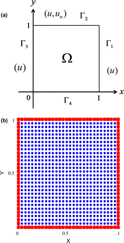
The computational domain for the first example is a square domain, which is shown in Figure 2(a). The whole boundary is denoted by $\mathit{\partial }\mathrm{\Omega }={\mathrm{\Gamma }}_1+{\mathrm{\Gamma }}_2+{\mathrm{\Gamma }}_3+{\mathrm{\Gamma }}_4$. The interior and boundary nodes are uniformly distributed inside the domain and along the boundary, which are demonstrated in Figure 2(b). The governing equation and the analytical solution for this example are:(24) $$\frac{{\mathit{\partial }}^{2}u}{\mathit{\partial }{x}^2}+2\frac{{\mathit{\partial }}^{2}u}{\mathit{\partial }{y}^2}+\frac{{\mathit{\partial }}^{2}u}{\mathit{\partial }x\mathit{\partial }y}+\frac{\mathit{\partial }u}{\mathit{\partial }x}-\frac{\mathit{\partial }u}{\mathit{\partial }y}=0,$$(24)

Figure 2. (a) The schematic diagram for example 1 and (b) the distributions of interior and boundary nodes.

and(25) $$u(x,y)=e^{x}cos(y).$$(25)

Dirichlet boundary conditions are given on ${\mathrm{\Gamma }}_1$ and ${\mathrm{\Gamma }}_3$. The over-specified boundary condition (Dirichlet and Neumann) is imposed on ${\mathrm{\Gamma }}_2$. There is no boundary condition on ${\mathrm{\Gamma }}_4$. These boundary conditions are obtained from the analytical solution, Equation (25). The following parameters are used in this example: $n_b=116$, $n_i=784$ and $n_s=12$.

In order to reflect realistic situations, different levels of noise are added into boundary conditions, Equations (2)–(5). Therefore, the boundary conditions will take the following forms:(26) $$u=f(x,y)\left(1+\frac{s}{100}\times rand\right)=e^{x}cos\left(y\right)\left(1+\frac{s}{100}\times rand\right),(x,y)\in {\mathrm{\Gamma }}_2,$$(26) (27) $$u_n=\left[\left(\mathrm{\nabla }u\right)·\overrightarrow{n}\right]\left(1+\frac{s}{100}\times rand\right)=g\left(x,y\right)\left(1+\frac{s}{100}\times rand\right)=\left[\mathrm{\nabla }\left(e^{x}cos\left(y\right)\right)·\overrightarrow{n}\right]\left(1+\frac{s}{100}\times rand\right),(x,y)\in {\mathrm{\Gamma }}_2,$$(27) (28) $$u=h(x,y)\left(1+\frac{s}{100}\times rand\right)=e^{x}cos\left(y\right)\left(1+\frac{s}{100}\times rand\right),(x,y)\in {\mathrm{\Gamma }}_1+{\mathrm{\Gamma }}_3,$$(28)

where $s$ is the percentage of added noise. rand is the random number and its range is $-1⩽rand⩽1$. The function RAND in MATLAB^® software is used in this paper to generate the noise.

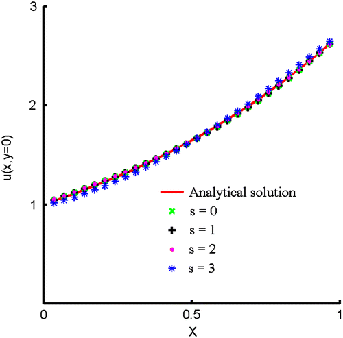
The numerical solutions, obtained by the GFDM, are shown in Figure 3. The analytical and numerical solutions are depicted by dashed lines and solid lines, respectively. From these two figures, it can be observed that the analytical and numerical results are almost identical. In Figure 3(a), there is no noise added into the boundary condition. On the other hand, the numerical solution, shown in Figure 3(b), is obtained by adding three-percent noise into the boundary conditions. Although s = 3% noise is added into the boundary conditions, the numerical solution is still very similar to the analytical solution. From Figure 3(b), it is obvious that the computational errors appear near the lower boundary, since there is no boundary condition imposed there. In order to carefully examine the results, the solutions along ${\mathrm{\Gamma }}_4$ are plotted in Figure 4. In this figure, the numerical solution along ${\mathrm{\Gamma }}_4$ is almost the same as the analytical solution even though different levels of noise are added. The maximum absolute errors obtained by adding different levels of noise are tabulated in Table 1 and the maximum absolute errors are very small. 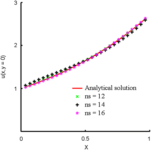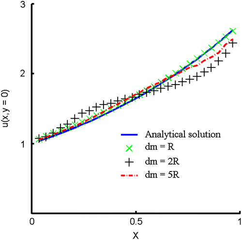Furthermore, the numerical results along ${\mathrm{\Gamma }}_4$, which are obtained by using different n_s, are depicted in Figure 5. It can be found that the numerical results are quite accurate with respect to the number of nodes in the star. Then, without changing the number of nodes in a star n_s = 12, the influence of the supporting radius of weighting function is examined by letting $d{m}_i=R_i$, $d{m}_i=2R_i$ and $d{m}_i=5R_i$ as shown in Figure 6. From the results in Figure 6, it is obvious that although the numerical solutions are very similar with the analytical solution, the supporting radius of weighting function still have influence on the numerical accuracy. From the provided results of this example, the accuracy and the stability of the GFDM for solving this two-dimensional Cauchy problem are verified.

Figure 3. The distributions of numerical (solid lines) and analytical solutions (dashed lines). (a) $s=0$ and (b) $s=3$.

Figure 4. The profiles of numerical solutions along ${\mathrm{\Gamma }}_4$ for example 1.

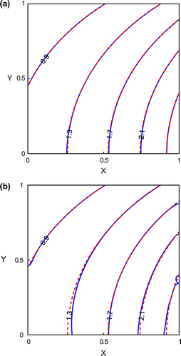
Table 1. The maximum absolute errors by adding different levels of noise for example 1.

Percentages of noise	Maximum absolute errors
s = 0	0.0118
s = 1	0.0242
s = 2	0.0510
s = 3	0.0806

Figure 5. The profiles of numerical solutions along ${\mathrm{\Gamma }}_4$ for example 1 (s = 3).

Figure 6. The profiles of numerical solutions along ${\mathrm{\Gamma }}_4$ by adopting different supporting radii of weighting function for example 1 (s = 3, $n_s=12$).

4.2 Example 2

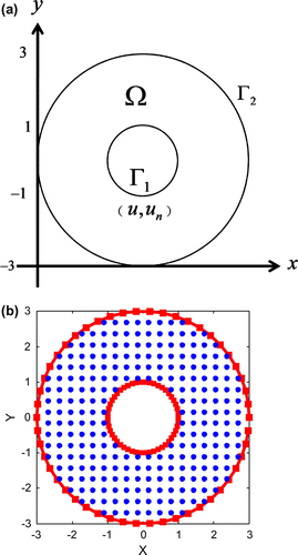
For the second validation problem, we used a doubly connected domain. The computational domain is a concentric annular domain, which is depicted in Figure 7(a). The radii for the two circular boundaries are 3 and 1. The governing equation and the analytical solution for this example are:(29) $$\frac{{\mathit{\partial }}^{2}u}{\mathit{\partial }{x}^2}+\frac{{\mathit{\partial }}^{2}u}{\mathit{\partial }{y}^2}=0,$$(29)

Figure 7. (a) The schematic diagram for example 2 and (b) the distributions of interior and boundary nodes.

and(30) $$u\left(x,y\right)=-\frac{1}{2}x+2y+\frac{1}{4}\left(x^2-y^2\right).$$(30)

There are two kinds of boundary conditions imposed on the inner boundary and no boundary condition is given on the outer boundary. The given boundary conditions are obtained from the analytical solution and the computational nodes are uniformly distributed inside the domain and along the boundary, which are displayed in Figure 7(b). There are 100 boundary nodes and 244 interior nodes used in this example. Besides, $n_s=16$ is used. The boundary conditions will take the following forms:(31) $$u=f(x,y)\left(1+\frac{s}{100}\times rand\right)=\left[-\frac{1}{2}x+2y+\frac{1}{4}\left(x^2-y^2\right)\right]\left(1+\frac{s}{100}\times rand\right),(x,y)\in {\mathrm{\Gamma }}_1,$$(31) (32) $$u_n=\left[\left(\mathrm{\nabla }u\right)·\overrightarrow{n}\right]\left(1+\frac{s}{100}\times rand\right)=g\left(x,y\right)\left(1+\frac{s}{100}\times rand\right)=\left[\mathrm{\nabla }\left(-\frac{1}{2}x+2y+\frac{1}{4}\left(x^2-y^2\right)\right)·\overrightarrow{n}\right]\left(1+\frac{s}{100}\times rand\right),(x,y)\in {\mathrm{\Gamma }}_1.$$(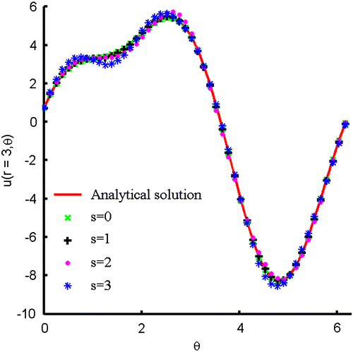32)

The numerical solutions with and without added noise are shown in Figure 8. In Figure 8(a), there is no noise added into the boundary conditions and the numerical solution (solid lines) is almost identical to the analytical solution (dashed lines). By adding three-percent noise into the boundary conditions, the numerical solution is slightly different from the analytical solution, depicted in Figure 8(b). The errors appeared near the outer boundary since there is no boundary condition given there. The solutions, obtained by adding different levels of noise, along the outer boundary are plotted in Figure 9. Three different levels of noise are added into the boundary conditions and the recovered boundary data are almost the same as the analytical solution, which can be seen in Figure 9. The maximum absolute errors obtained by adding different levels of noise are tabulated in Table 2 and they are very small.

Figure 8. The distributions of numerical (solid lines) and analytical solutions (dashed lines). (a) $s=0$ and (b) $s=3$.

Figure 9. The profiles of numerical solutions along ${\mathrm{\Gamma }}_2$ for example 2.

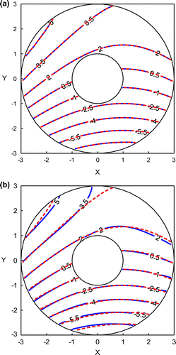
Table 2. The maximum absolute errors by adding different levels of noise for example 2.

Percentages of noise	Maximum absolute errors
s = 0	7.7658 × 10^−12
s = 1	0.0806
s = 2	0.3427
s = 3	0.5077

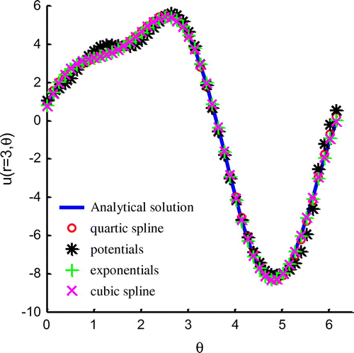
Since from previous researches [27,28] there are some choices of the weighting functions, we adopted the following weighting functions to validate the accuracy of numerical results:(33) $$\text{potential:}w\left(d_{ij}\right)=\frac{1}{d_{ij}^3},$$(33) (34) $$\text{exponential:}w\left(d_{ij}\right)=e^{-5d_{ij}^2},$$(34) (35) $$\text{cubic spline:}w\left(d_{ij}\right)=\left\{\begin{array}{cc}\frac{2}{3}-4{\left(\frac{d_{ij}}{d{m}_i}\right)}^2+4{\left(\frac{d_{ij}}{d{m}_i}\right)}^3\hfill & 0⩽d_{ij}⩽\frac{d{m}_i}{2}\hfill \\ \frac{3}{4}-4\left(\frac{d_{ij}}{d{m}_i}\right)+4{\left(\frac{d_{ij}}{d{m}_i}\right)}^2-\frac{4}{3}{\left(\frac{d_{ij}}{d{m}_i}\right)}^3\hfill & \frac{d{m}_i}{2}<d_{ij}⩽d{m}_i\hfill \\ 0\hfill & d{m}_i<d_{ij}\hfill \end{array}\right..$$(35)

The profiles of numerical results along the under-specified boundary are depicted in Figure 10. The numerical results, obtained by using noisy boundary data and different weight functions, are very similar with the analytical solution. Among them, only the solutions by using potential function, Equation (33), as weighting function show obvious errors in this figure. Hence, it can be found that the numerical results of the GFDM are quite stable with respect to different weighting functions. From these provided comparisons, the stability and the accuracy of the GFDM for solving inverse problem are demonstrated again.

Figure 10. The profiles of numerical solutions along ${\mathrm{\Gamma }}_2$ by adopting different weighting functions for example 2.

4.3 Example 3

For the third example, a square domain is considered and the computational nodes are uniformly distributed. The governing equation is(36) $$\frac{{\mathit{\partial }}^{2}u}{\mathit{\partial }{x}^2}+\frac{{\mathit{\partial }}^{2}u}{\mathit{\partial }{y}^2}+\left(2-x^2-y^2\right)\frac{{\mathit{\partial }}^{2}u}{\mathit{\partial }x\mathit{\partial }y}+e^{x-y}\frac{\mathit{\partial }u}{\mathit{\partial }x}=-e^{x-y}.$$(36)

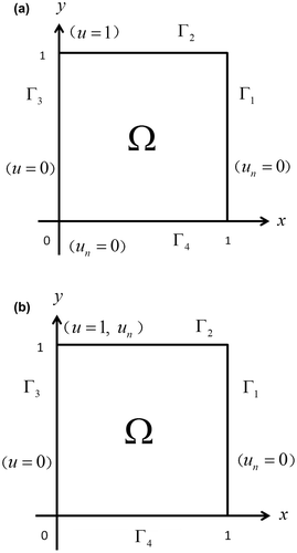
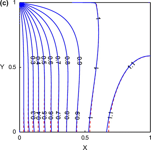
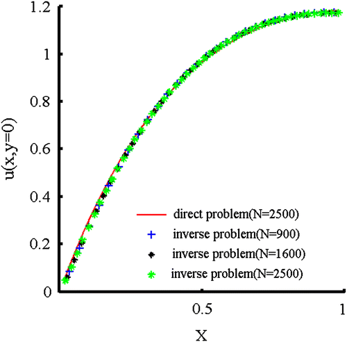
The boundary conditions for the direct problem are shown in Figure 11(a). In the direct problem, one boundary condition is imposed on each boundary segment. It is nontrivial to find the analytical solution by mathematical means. We first used the GFDM to solve the direct problem. Then, the obtained Neumann data along the upper boundary are imposed along there and the original boundary condition along the lower boundary segment is removed. Therefore, an inverse Cauchy problem will be formed by following this procedure, which is demonstrated in Figure 11(b). The GFDM is applied to this inverse Cauchy problem. Since the numerical solution from the direct problem will contain numerical errors, we do not have to add extra noise into the boundary conditions for the inverse problem. The numerical solutions from the direct and the inverse problems will be compared with each other to show the accuracy of the solutions.

Figure 11. The schematic diagrams for example 3. (a) Direct problem and (b) inverse problem.

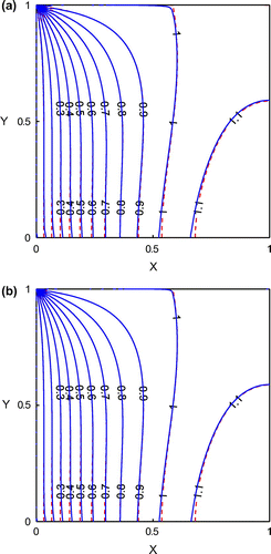
The distributions of numerical solutions from the direct problem (dashed lines) and the inverse problem (solid lines) are shown in Figure 12. In this figure, three different numbers of nodes (N) are used. No matter what number of nodes is used, the solutions from the direct problem and the inverse problem are almost identical. These results show the stability of the GFDM for solving this inverse Cauchy problem. Since there is no boundary condition along the lower boundary, the solutions along the lower boundary using different numbers of nodes are plotted in Figure 13. From the figure, it is obvious that these solutions are almost identical to the results of the direct problem.

Figure 12. The distributions of numerical solutions from the direct problem (dashed lines) and the inverse problem (solid lines). (a) N = 900 (b) N = 1600 and (c) N = 2500.

Figure 13. The profiles of numerical solutions along ${\mathrm{\Gamma }}_4$ for example 3.

5. Conclusions

In this paper, the GFDM is adopted for solving inverse Cauchy problems, governed by second-order linear partial differential equations. The GFDM is a newly developed domain-type meshless method which is free from mesh generation and numerical quadrature. In Cauchy problems, part of the boundary data is missing and the numerical simulation may become very unstable. Small errors in the boundary conditions will greatly decrease the accuracy of the results. For this reason, we tested the stability and the accuracy of the GFDM for solving such problems.

There are three numerical examples in the paper which show the excellent performance of the GFDM for solving inverse problems. This meshless method can be used for the solution of inverse problems in simply connected and doubly connected domains. Besides, different levels of noise (s = 1, s = 2, s = 3) are added into the boundary conditions to demonstrate the stability of the GFDM. In the third example, a direct problem is solved and then we used the obtained extra boundary data to form an inverse problem. The numerical solutions from the direct and the inverse problems are almost the same, which show the stability of the GFDM. From the numerical experiments in this paper, the stability, the accuracy and the simplicity of the GFDM for solving two-dimensional Cauchy problems are verified.

References

- Fu Z, Chen W, Zhang C. Boundary particle method for Cauchy inhomogeneous potential problems. Inverse Probl. Sci. Eng. 2012;20:189–207.10.1080/17415977.2011.603085
- Zhou D, Wei T. The method of fundamental solutions for solving a Cauchy problem of Laplace's equation in a multi-connected domain. Inverse Probl. Sci. Eng. 2008;16:389–411.10.1080/17415970701602614
- Lesnic D, Elliott L, Ingham DB. A alternating boundary element method for solving Cauchy problems for the biharmonic equation. Inverse Probl. Eng. 1997;5:145–168.10.1080/174159797088027657
- Fan CM, Chan HF. Modified collocation Trefftz method for the geometry boundary identification problem of heat conduction. Numer. Heat Transfer B-Fundam. 2011;59:58–75.10.1080/10407790.2010.541355
- Chan HF, Fan CM, Yeih W. Solution of inverse boundary optimization problem by Trefftz method and exponentially convergent scalar homotopy algorithm. CMC – Comput. Mat. Contin. 2011;24:125–142.
- Karageorghis A, Lesnic D. Detection of cavities using the method of fundamental solutions. Inverse Probl. Sci. Eng. 2009;17:803–820.10.1080/17415970802580263
- Karageorghis A, Lesnic D, Marin L. Regularized collocation Trefftz method for void detection in two-dimensional steady-state heat conduction problems. Inverse Probl. Sci. Eng. 2014;22:395–418.10.1080/17415977.2013.788172
- Lesnic D, Elliott L, Ingham DB. An iterative boundary element method for solving numerically the Cauchy problem for the Laplace equation. Eng. Anal. Bound. Elem. 1997;20:123–133.10.1016/S0955-7997(97)00056-8
- Liu CS, Atluri SN. Numerical solution of the Laplacian Cauchy problem by using a better postconditioning collocation Trefftz method. Eng. Anal. Bound. Elem. 2013;37:74–83.10.1016/j.enganabound.2012.08.008
- Fu CL, Li HF, Qian Z, Xiong XT. Fourier regularization method for solving a Cauchy problem for the Laplace equation. Inverse Probl. Sci. Eng. 2008;16:159–169.10.1080/17415970701228246
- Young DL, Tsai CC, Chen CW, Fan CM. The method of fundamental solutions and condition number analysis for inverse problems of Laplace equation. Comput. Math. Appl. 2008;55:1189–1200.10.1016/j.camwa.2007.05.015
- Karageorghis A, Lesnic D, Marin L. A survey of applications of the MFS to inverse problems. Inverse Probl. Sci. Eng. 2011;19:309–336.10.1080/17415977.2011.551830
- Fan CM, Chan HF, Kuo CL, Yeih W. Numerical solutions of boundary detection problems using modified collocation Trefftz method and exponentially convergent scalar homotopy algorithm. Eng. Anal. Bound. Elem. 2012;36:2–8.10.1016/j.enganabound.2010.12.008
- Fan CM, Li HH. Solving the inverse Stokes problems by the modified collocation Trefftz method and Laplacian decomposition. Appl. Math. Comput. 2013;219:6520–6535.10.1016/j.amc.2012.12.081
- Fan CM, Liu YC, Chan HF, Hsiao SS. Solutions of boundary detection problem for modified Helmholtz equation by Trefftz method. Inverse Probl. Sci. Eng. 2014;22:267–281.10.1080/17415977.2013.773325
- Chen CS, Fan CM, Wen PH. The method of approximate particular solutions for solving elliptic problems with variable coefficients. Int. J. Comput. Methods. 2011;8:545–559.10.1142/S0219876211002484
- Chen CS, Fan CM, Wen PH. The method of approximate particular solutions for solving certain partial differential equations. Numer. Meth. Part Differ. Equ. 2012;28:506–522.10.1002/num.v28.2
- Divo E, Kassab AJ. Localized meshless modeling of natural-convective viscous flows. Numer. Heat Transfer B-Fundam. 2008;53:487–509.10.1080/10407790802083190
- Kosec G, Sarler B. Local RBF collocation method for Darcy flow. CMES – Comp. Model. Eng. Sci. 2008;25:197–207.
- Fan CM, Chien CS, Chan HF, Chiu CL. The local RBF collocation method for solving the double-diffusive natural convection in fluid-saturated porous media. Int. J. Heat Mass Transfer. 2013;57:500–503.10.1016/j.ijheatmasstransfer.2012.10.044
- Chan HF, Fan CM. The local radial basis function collocation method for solving two-dimensional inverse Cauchy problems. Numer. Heat Transfer B-Fundam. 2013;63:284–303.10.1080/10407790.2013.772004
- Mramor K, Vertnik R, Sarler B. Low and intermediate Re solution of lid driven cavity problem by local radial basis function collocation method. CMC – Comput. Mat. Contin. 2013;36:1–21.
- Li M, Chen W, Chen CS. The localized RBFs collocation methods for solving high dimensional PDEs. Eng. Anal. Bound. Elem. 2013;37:1300–1304.10.1016/j.enganabound.2013.06.001
- Kelly JM, Divo EA, Kassab AJ. Numerical solution of the two-phase incompressible Navier–Stokes equations using a GPU-accelerated meshless method. Eng. Anal. Bound. Elem. 2014;40:36–49.10.1016/j.enganabound.2013.11.015
- Sadat H, Prax C. Application of the diffuse approximation for solving fluid flow and heat transfer problems. Int. J. Heat Mass Transfer. 1996;39:214–218.10.1016/S0017-9310(96)85018-6
- Sadat H, Dubus N, Gbahoué L, Sophy T. On the solution of heterogeneous heat conduction problems by a diffuse approximation meshless method. Numer. Heat Transfer B-Fundam. 2006;50:491–498.10.1080/10407790600710184
- Benito JJ, Ureña F, Gavete L. Influence of several factors in the generalized finite difference method. Appl. Math. Model. 2001;25:1039–1053.10.1016/S0307-904X(01)00029-4
- Gavete L, Gavete ML, Benito JJ. Improvements of generalized finite difference method and comparison with other meshless method. Appl. Math. Model. 2003;27:831–847.10.1016/S0307-904X(03)00091-X
- Ureña F, Benito JJ, Salete E, Gavete L. A note on the application of the generalized finite difference method to seismic wave propagation in 2D. J. Comput. Appl. Math. 2012;236:3016–3025.10.1016/j.cam.2011.04.005
- Ureña F, Salete E, Benito JJ, Gavete L. Solving third- and fourth-order partial differential equations using GFDM: application to solve problems of plates. Int. J. Comput. Math. 2012;89:366–376.10.1080/00207160.2011.587871
- Chan HF, Fan CM, Kuo CW. Generalized finite difference method for solving two-dimensional non-linear obstacle problems. Eng. Anal. Bound. Elem. 2013;37:1189–1196.10.1016/j.enganabound.2013.05.004
- Tsai CH, Kolibal J, Li M. The golden section search algorithm for finding a good shape parameter for meshless collocation methods. Eng. Anal. Bound. Elem. 2010;34:738–746.10.1016/j.enganabound.2010.03.003
- Ling L, Schaback R. An improved subspace selection algorithm for meshless collocation methods. Int. J. Numer. Meth. Eng. 2009;80:1623–1639.10.1002/nme.v80:13
- Ling L, Kansa EJ. A least-squares preconditioner for radial basis functions collocation methods. Adv. Comput. Math. 2005;23:31–54.10.1007/s10444-004-1809-5