Inverse calculation of elastic moduli in cross-anisotropic and layered pavements by system identification method

Abstract

Material properties of cross-anisotropic (or transversely isotropic) elastic and layered systems including pavement structures are essential for the analysis of mechanical responses. Besides laboratory determination of these material properties, direct inversion using in situ input data is fundamental and more useful. In this paper, the system identification (SID) method with constraints is proposed to invert the elastic moduli in an anisotropic layered half space in general and in a layered pavement in particular. Since in the inverse calculation, the forward calculation is required, we have also presented briefly the forward calculation approach based on the cylindrical system of vector functions and the propagating matrix method. Our SID algorithm is then applied to three-layer and four-layer pavements with different numbers of cross-anisotropic layers, with the deflections at the surface of the layered pavement as inputs. Our numerical results demonstrate clearly that the proposed SID-based inverse method is accurate and efficient for a broad range of seed moduli.

Keyword:

• inverse problem
• layered pavement
• cross-anisotropy (transverse isotropy)
• system identification

1. Introduction

Anisotropic and layered materials and structures are very common in different engineering fields. For instance, it was observed that the behaviour of pavement materials including asphalt concrete, unbound granular base and subgrade soils would be anisotropic due to the preferred orientation of the aggregates which widely exist in the pavement materials.[1–7] Using the micromechanical analysis and experimental techniques, Masad and his colleagues demonstrated that the asphalt mix behaved as an anisotropic material.[1] Underwood et al. tested and studied the anisotropy of asphalt concrete cores in the vertical and horizontal directions from gyratory-compacted specimens.[2] Wagoner and Braham investigated the anisotropic effect at low temperatures for samples compacted with superpave gyratory compactor.[3] Zhang et al. analyzed the inherent anisotropy of asphalt mixture in microstructure, and showed experimentally that the magnitude of the compressive stiffness in the vertical direction was 1.2 to 2 times that in the horizontal direction.[4] The anisotropic properties of unbound granular base were investigated using several experimental techniques including the triaxial loading test.[5,6] The non-linear and anisotropic behaviour of unbound granular base was also investigated.[7] Therefore, consideration of the cross-anisotropic behaviour is necessary in the mechanistic analysis of layered pavement structures.

For the best performance of the structures, it is crucial that the material properties and their behaviour are well understood. While one could determine the material properties by conducting laboratory tests, the results obtained may not accurately present the actual or in situ material properties. As such, inverse problems are important topics in structural and materials engineering.[8–11] For example, the generalized extremal algorithm was applied for the solution of an inverse problem in order to estimate the material properties [8] and the obtained results indicated that this algorithm was competitive with other stochastic methods such as genetic algorithms. Using an analytical inverse technique, the structural characteristics of a beam were modelled by Moaveni and Chou and the comparison of their results with the direct solutions confirms the capability of the inverse method.[10] Recently, Messineo et al. developed an inverse problem for ultrasonic transmission through multilayer systems.[11] In addition, the use of modelling techniques such as finite element and boundary element methods together with inverse problems and minimization techniques has been constantly a research topic.[12,13]

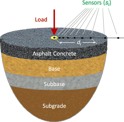
In pavement engineering, evaluation of the material properties or the pavement moduli can be performed by different in situ methods such as the plate bearing test, multi-depth deflectometers and falling weight deflectometers (FWD) (Figure 1). Estimation of the pavement material properties from FWD test data is very popular among pavement engineers and based on that several methods have been developed to backcalculate the mechanical properties.[14,15] For instance, the pavement backcalculation procedure can be conducted using different iteration methods including the gradient search, intelligent optimization [16], hybrid schemes [17] and evolutionary algorithms.[18] So far, however, no inverse algorithm has been proposed for the backcalculation of pavement properties where each layer could be of cross-anisotropy.

Figure 1. Schematics of the FWD for measuring the surface deflections of a layered pavement at sensors s_i with distances d_i from the loading centre.

In this paper, the system identification method (SID) is proposed to invert the elastic moduli in cross-anisotropic and layered pavements. The input data for the inversion of material properties are the deflections on the surface of the layered pavements which can be observed using the FWD and which will be mimicked in this paper via our forward algorithm. This paper is organized as follows. In Section 2, we present the forward algorithm for solving the cross-anisotropic layered pavements. In Section 3, the SID method with constraints will be presented. In Section 4, numerical examples on the inverted material properties based on the SID approach are given for different layered pavements. Conclusions are drawn in Section 5.

2. Forward solutions in cross-anisotropic multilayered media

We consider a homogeneous but cross-anisotropic layer with its axis of symmetry being along the z-axis. Then the equilibrium equations in the cylindrical coordinate system (r, θ, z) can be expressed as(1) $$\begin{array}{c}\frac{\mathit{\partial }{\mathit{\sigma }}_{rr}}{\mathit{\partial }r}+\frac{\mathit{\partial }{\mathit{\sigma }}_{r\mathit{\theta }}}{r\mathit{\partial }\mathit{\theta }}+\frac{\mathit{\partial }{\mathit{\sigma }}_{rz}}{\mathit{\partial }z}+\frac{{\mathit{\sigma }}_{rr}-{\mathit{\sigma }}_{\mathit{\theta }\mathit{\theta }}}{r}=0\hfill \\ \hfill \\ \frac{\mathit{\partial }{\mathit{\sigma }}_{r\mathit{\theta }}}{\mathit{\partial }r}+\frac{\mathit{\partial }{\mathit{\sigma }}_{\mathit{\theta }\mathit{\theta }}}{r\mathit{\partial }\mathit{\theta }}+\frac{\mathit{\partial }{\mathit{\sigma }}_{\mathit{\theta }z}}{\mathit{\partial }z}+\frac{2{\mathit{\sigma }}_{r\mathit{\theta }}}{r}=0\hfill \\ \hfill \\ \frac{\mathit{\partial }{\mathit{\sigma }}_{rz}}{\mathit{\partial }r}+\frac{\mathit{\partial }{\mathit{\sigma }}_{\mathit{\theta }z}}{r\mathit{\partial }\mathit{\theta }}+\frac{\mathit{\partial }{\mathit{\sigma }}_{zz}}{\mathit{\partial }z}+\frac{{\mathit{\sigma }}_{rz}}{r}=0\hfill \\ \hfill \end{array}$$(1)

where σ_ij are the components of the stress tensor. Also in the cylindrical coordinate system, the constitutive relations can be written, for the layer of cross-anisotropy with z being the axis of symmetry, as(2) $$\begin{array}{c}{\mathit{\sigma }}_{rr}=c_{11}{\mathit{\gamma }}_{rr}+c_{12}{\mathit{\gamma }}_{\mathit{\theta }\mathit{\theta }}+c_{13}{\mathit{\gamma }}_{zz}\hfill \\ {\mathit{\sigma }}_{\mathit{\theta }\mathit{\theta }}=c_{12}{\mathit{\gamma }}_{rr}+c_{11}{\mathit{\gamma }}_{\mathit{\theta }\mathit{\theta }}+c_{13}{\mathit{\gamma }}_{zz}\hfill \\ {\mathit{\sigma }}_{zz}=c_{13}{\mathit{\gamma }}_{rr}+c_{13}{\mathit{\gamma }}_{\mathit{\theta }\mathit{\theta }}+c_{33}{\mathit{\gamma }}_{zz}\hfill \\ {\mathit{\sigma }}_{\mathit{\theta }z}=2c_{44}{\mathit{\gamma }}_{\mathit{\theta }z};{\mathit{\sigma }}_{rz}=2c_{44}{\mathit{\gamma }}_{rz};{\mathit{\sigma }}_{r\mathit{\theta }}=2c_{66}{\mathit{\gamma }}_{r\mathit{\theta }}\hfill \end{array}$$(2)

where γ_ij are the components of the strain tensor and c_ij are the elastic constants. It is noted that since c₆₆ = (c₁₁–c₁₂)/2, there are only five independent elastic constants in Equation (2). Furthermore, in many engineering fields, particularly in pavement engineering, the five elastic constants c_ij are usually expressed in terms of the five engineering coefficients as expressed below:(3) $$\begin{array}{c}{c}_{11}=\frac{E_h\left[1-(E_h/E_v)\right]{\mathit{\mu }}_v^2}{(1+{\mathit{\mu }}_h)\left[1-{\mathit{\mu }}_h-(2E_h/E_v){\mathit{\mu }}_v^2\right]}\hfill \\ c_{12}=\frac{E_h\left[{\mathit{\mu }}_h+(E_h/E_v){\mathit{\mu }}_v^2\right]}{(1+{\mathit{\mu }}_h)\left[1-{\mathit{\mu }}_h-(2E_h/E_v){\mathit{\mu }}_v^2\right]}\hfill \\ c_{13}=\frac{E_h{\mathit{\mu }}_v}{1-{\mathit{\mu }}_h-(2E_h/E_v){\mathit{\mu }}_v^2};c_{33}=\frac{E_v(1-{\mathit{\mu }}_h)}{1-{\mathit{\mu }}_h-(2E_h/E_v){\mathit{\mu }}_v^2}\hfill \\ c_{44}=G_v;\begin{array}{cc}& c_{66}\equiv \frac{c_{11}-c_{12}}{2}=\frac{E_h}{2(1+{\mathit{\mu }}_h)}\end{array}\hfill \end{array}$$(3)

where E_h and E_v are the Young’s moduli within the plane of transverse isotropy and normal to it, respectively; μ_h and μ_v are the Poisson’s ratios characterizing the lateral strain response in the plane of transverse isotropy relative to the in-plane strain and the strain normal to it, respectively; and G_v is the shear modulus in the plane normal to the plane of transverse isotropy.

It should be noted that since the strain energy should be always positive in an elastic solid, all principal minors of the stiffness matrix [c_ij] in Equation (2) must be positive.[19] This leads to the following constraints on the five engineering coefficients.(4) $$\begin{array}{c}{E}_v,E_h,G_v>0\hfill \\ -1<{\mathit{\mu }}_h<1\hfill \\ -\sqrt{\frac{E_v}{E_h}·\frac{1-{\mathit{\mu }}_h}{2}}<{\mathit{\mu }}_v<\sqrt{\frac{E_v}{E_h}·\frac{1-{\mathit{\mu }}_h}{2}}\hfill \end{array}$$(4)

As it is well known, besides the equilibrium equations in Equation (1) and the constitutive relations in Equation (2), we also need the strain-displacement relations. In the cylindrical coordinate system, the components of the strain tensor are related to the three elastic displacements u_i by(5) $$\begin{array}{c}{\mathit{\gamma }}_{rr}=\frac{\mathit{\partial }{u}_r}{\mathit{\partial }r};{\mathit{\gamma }}_{\mathit{\theta }\mathit{\theta }}=\frac{\mathit{\partial }{u}_{\mathit{\theta }}}{r\mathit{\partial }\mathit{\theta }}+\frac{u_r}{r};{\mathit{\gamma }}_{zz}=\frac{\mathit{\partial }{u}_z}{\mathit{\partial }z}\hfill \\ {\mathit{\gamma }}_{\mathit{\theta }z}=\frac{1}{2}\left(\frac{\mathit{\partial }{u}_{\mathit{\theta }}}{\mathit{\partial }z}+\frac{\mathit{\partial }{u}_z}{r\mathit{\partial }\mathit{\theta }}\right);{\mathit{\gamma }}_{rz}=\frac{1}{2}\left(\frac{\mathit{\partial }{u}_z}{\mathit{\partial }r}+\frac{\mathit{\partial }{u}_r}{\mathit{\partial }z}\right);{\mathit{\gamma }}_{r\mathit{\theta }}=\frac{1}{2}\left(\frac{\mathit{\partial }{u}_r}{r\mathit{\partial }\mathit{\theta }}+\frac{\mathit{\partial }{u}_{\mathit{\theta }}}{\mathit{\partial }r}-\frac{u_{\mathit{\theta }}}{r}\right)\hfill \end{array}$$(5)

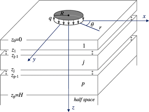
With the governing Equations (1), (2) and (5) for a cross-anisotropic elastic layer, we now describe the corresponding boundary value problem for the layered half space. We assume now that there is a p-layered cross-anisotropic elastic half space with perfectly bonded interfaces. The layers are numbered consecutively with the layer at the top being layer 1 and the last layer being layer p, which is just above the half space (Figure 2). We place the cylindrical coordinates on the surface with the z-axis pointing into the layered half space. The jth layer is bounded by the interfaces z = z_j−1, z_j with z_j−1 being the vertical coordinate of the upper interface of the jth layer and z_j being that of the lower interface. It is obvious that z₀ = 0 and z_p = H, where H is the depth of the last layer interface. Also for the jth layer, its thickness is h_j = z_j – z_j−1. We assume that there is a vertical load uniformly applied over a circular area (r < R) on the surface of this p-layered half space with magnitude q, as shown in Figure 2. Then, the boundary conditions on the surface of the layered half space can be expressed as(6) $$\begin{array}{c}{\mathit{\sigma }}_{zz}=\left\{\begin{array}{cc}-q\hfill & 0⩽r⩽R\\ 0\hfill & r>R\end{array}\right.\\ {\mathit{\sigma }}_{rz}={\mathit{\sigma }}_{\mathit{\theta }z}=0\end{array}$$(6)

Figure 2. Schematics of a p-layered pavement half space under a uniform vertical loading q within the circle r = R on the surface.

The forward problem in such a layered half space is to find the solutions of displacement, strain and stress fields at any observation point induced by the surface loading (Equation (6)). The solution should obviously satisfy the boundary conditions on the surface, the interface continuity conditions along the interfaces (i.e. the elastic displacements u_i and the stress components σ_iz should be continuous across the interfaces); and the solutions should decay to zero as the observation point approaches infinity.

A couple of useful approaches have been proposed to solve the forward problem of layered half spaces under a vertical surface loading within a circle of r = R, (i.e. [20,21]). In this paper, we only briefly mention the vigorous analytical method [22,23] by Pan since our inverse algorithm will be based on this forward calculation. The method in [22,23] is based on the propagator matrix method in terms of the cylindrical system of vector functions with the latter being defined as(7a) $$\begin{array}{c}\mathit{L}(r,\mathit{\theta };\mathit{\lambda },m)={\mathit{e}}_{z}S(r,\mathit{\theta };\mathit{\lambda },m)\hfill \\ \mathit{M}(r,\mathit{\theta };\mathit{\lambda },m)=\left({\mathit{e}}_r\frac{\mathit{\partial }}{\mathit{\partial }r}+{\mathit{e}}_{\mathit{\theta }}\frac{\mathit{\partial }}{r\mathit{\partial }\mathit{\theta }}\right)S(r,\mathit{\theta };\mathit{\lambda },m)\hfill \\ \mathit{N}(r,\mathit{\theta };\mathit{\lambda },m)=\left({\mathit{e}}_r\frac{\mathit{\partial }}{r\mathit{\partial }\mathit{\theta }}-{\mathit{e}}_{\mathit{\theta }}\frac{\mathit{\partial }}{\mathit{\partial }r}\right)S(r,\mathit{\theta };\mathit{\lambda },m)\hfill \end{array}$$(7a)

where e_r, e_θ and e_z are the unit vectors along the coordinate axes r, θ and z, respectively, and(7b) $$S(r,\mathit{\theta };\mathit{\lambda },m)=\frac{1}{\sqrt{2\mathit{\pi }}}{J}_m(\mathit{\lambda }r)e^{im\mathit{\theta }};m=0,\pm 1,\pm 2,\dots$$(7b)

with J_m(λr) being the Bessel function of order m (m = 0 corresponds to the axial symmetric deformation) and i = $\sqrt{-1}$. The parameters λ and m are the transformation variables corresponding to the horizontal physical variables r and θ, respectively.

Due to the orthogonality of the vector functions in Equation (7a), any vector, such as the displacement and traction vectors, at any z-level can be expressed as follows:(8a) $$\mathit{u}(r,\mathit{\theta },z)=\sum _m{\int }_0^{+\infty }[U_L(z)\mathit{L}(r,\mathit{\theta })+U_M(z)\mathit{M}(r,\mathit{\theta })+U_N(z)\mathit{N}(r,\mathit{\theta })]\mathit{\lambda }d\mathit{\lambda }$$(8a) (8b) $$\mathit{t}(r,\mathit{\theta },z)\equiv {\mathit{\sigma }}_{rz}{\mathit{e}}_r+{\mathit{\sigma }}_{\mathit{\theta }z}{\mathit{e}}_{\mathit{\theta }}+{\mathit{\sigma }}_{zz}{\mathit{e}}_z=\sum _m{\int }_0^{+\infty }[T_L(z)\mathit{L}(r,\mathit{\theta })+T_M(z)\mathit{M}(r,\mathit{\theta })+T_N(z)\mathit{N}(r,\mathit{\theta })]\mathit{\lambda }d\mathit{\lambda }$$(8b)

The in-plane stress components can be obtained using these equations and the constitutive relations in Equation (2). Making use of these relations and carrying out some simple mathematical operations, one can arrive at the following ordinary differential equations for the expansion coefficients in Equation (8) in each layer.[22]$$d{U}_L/dz={\mathit{\lambda }}^2{U}_M{c}_{13}/c_{33}+T_L/c_{33}$$$$d{U}_M/dz=-U_L+T_M/c_{44}$$$$d{T}_L/dz={\mathit{\lambda }}^2{T}_M$$(9a) $$d{T}_M/dz={\mathit{\lambda }}^2{U}_M(c_{11}{c}_{33}-c_{13}^2)/c_{33}-c_{13}{T}_L/c_{33}$$(9a) (9b) $$\begin{array}{c}d{U}_N/dz=T_N/c_{44}\hfill \\ d{T}_N/dz={\mathit{\lambda }}^2{c}_{66}{U}_N\hfill \end{array}$$(9b)

In our forward and inverse calculations of the layered system under the uniform vertical load within a circular area on the surface (Equation (6) and Figure 2), the deformation will be axis-symmetric. Thus, the solution related to Equation (9b) will be automatically zero and it will not be discussed thereafter. Furthermore, due to the symmetric feature, our solution should be independent of variable θ. In other words, ∂f/∂θ = 0 for any physical quantity f and thus we only need m = 0 in Equation (7) for the involved cylindrical function S.

From Equation (9a), one can easily find the solution matrix [Z(z)] in each layer and thus the corresponding propagator matrix [a(z)] between the top z_j−1 and bottom z_j interfaces (Figure 2) of any layer j as [22,23](10a) $$[E(z)]=[Z(z)][K]$$(10a) (10b) $$[E(z_{j-1})]=[a(z_j-z_{j-1})][E(z_j)]$$(10b)

where [E(z)] is the expansion coefficient column matrix defined by(11) $$[E(z)]={[U_L(z),\mathit{\lambda }{U}_M(z),T_L(z)/\mathit{\lambda },T_M(z)]}^T$$(11)

and [K] is a 4 × 1 column coefficient matrix with its elements to be determined by the continuity and/or boundary conditions. It is also noticed that Equation (10b) can be propagated from one layer to the other repeatedly so that the unknown coefficients [K] in Equation (10a) in the bottom homogeneous half space and the tractions on the surface of the layered half space can be connected and solved. It is noted that in the bottom homogeneous half space, two of the coefficients in [K] should be zero since the solution in the half space has to decay to zero when z approaches infinity. On the surface of the layered half space, the expansion coefficients for the traction vector in Equation (8b) can be found (making use of the boundary condition in Equation (6)) as(12) $$T_L(\mathit{\lambda };0)=\frac{1}{\sqrt{2\mathit{\pi }}}\underset{0}{\overset{2\mathit{\pi }}{\int }}\underset{0}{\overset{R}{\int }}-q{J}_0(\mathit{\lambda }r)rdrd\mathit{\theta }=-\sqrt{2\mathit{\pi }}R{J}_1(R\mathit{\lambda })q/\mathit{\lambda };T_M(\mathit{\lambda };0)=0$$(12)

After solving these four unknowns, two on the surface and two in the homogeneous half space, the propagator relation (10b) can be propagated to any z-level to find the expansion coefficients there. Thus, the solutions in terms of the cylindrical system of vector functions can be found at any z-level. With these expansion coefficients, the physical-domain solutions can be obtained by carrying out the inverse transform, which can be carried out numerically.[22,24] Therefore, the forward problem has been successfully solved. In the next section, we discuss the corresponding inverse method in a layered half space.

3. Inversion solutions in cross-anisotropic multilayered media

In pavement engineering, a layered pavement is mostly investigated by the FWD-related methods. In terms of the FWD, a uniform vertical loading is applied within a circle on the surface of the layered pavement (Figure 1). Then the surface deflections (i.e. u_z) will be measured by either seven or nine sensors located on the surface as the FWD standard. In this paper, we assume that there are nine sensors on the surface in the FWD. While the measured deflections can be directly applied to analyze the pavement behaviour, they can also be utilized to invert the material parameters in the layered pavements. The approach associated with the latter is called backcalculation (or inversion) algorithm in pavement engineering.

While a couple of methods have been proposed to backcalculate the elastic moduli in layered pavements (or half spaces), most of those methods are restricted to very small number of layers, to narrow seed moduli and to elastic isotropy.[14,15,18,25] Backcalculation of cross-anisotropic and layered half spaces using the FWD data has not been reported in the literature.

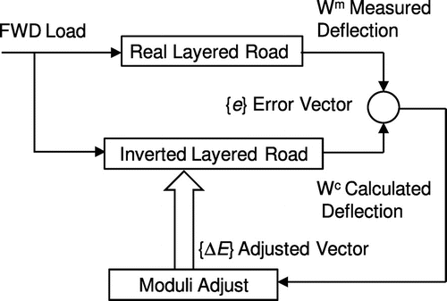
In this paper, we propose the SID method to invert the cross-anisotropic moduli of a layered pavement half space. The SID method was originally introduced by Wang and Lytton to invert the modulus and thickness of isotropic elastic-layered pavements [26] and later by Lytton to analyze the subsurface radar signals.[27] The principle of this method is based on the Taylor’s series expansion of a non-periodic function combined with an iterative scheme as shown in Figure 3.

Figure 3. Schematics of the SID method in moduli inversion of layered pavements using the FWD-measured surface deflections as inputs.

In the SID inverse process, the deflections at the nine sensors measured by the FWD are used as the inputs to backcalculate the moduli in each layer of the pavement. The thickness and Poisson’s ratio of each layer are fixed as given. The adjusted moduli vector {ΔE} (including the Young’s and shear moduli in all layers) is then obtained in an iterative process and is controlled by the following equation.(13) $$\left[F\right]·\left\{\mathrm{\Delta }E\right\}=\left\{e\right\}$$(13)

where the symbol “[]” is for a matrix and “{}” for a vector. Also in Equation (13), {e} is the relative error vector of the surface deflection between the calculated and measured ones with its element being defined as(14) $$e_i=W_i^m-W_i^c$$(14)

where ${W_i}^m$ is the measured deflection at ith sensor location by the FWD and ${W_i}^c$ the calculated deflection at the same sensor location (i = 1 − m, with m being the total number of the sensors in FWD, which is 9 in the present study). The elements of the sensitivity matrix [F] in Equation (13) is defined as(15) $$F_{ij}=\frac{\mathit{\partial }{W_i}^c}{\mathit{\partial }{E}_j}$$(15)

where E_j is the modulus in the inverse procedure (j = 1 − n, with n being the total number of moduli to be backcalculated, which varies from four to eight in the present study).

It should be pointed out that since total number of rows (i.e. the number of sensors) m is usually not the same as the total number of columns (i.e. the number of unknown moduli) n (m ≥ n in general and it is also true in the present study), the linear system of algebraic equations (13) is not a regular one where m = n. Furthermore, the coefficient matrix, i.e. the sensitivity matrix [F] in Equation (13), could be ill-conditioned when two or more moduli have similar effects on, or when a modulus has a negligible effect on, the behaviour of the layered pavement. Thus, in order to solve ΔE_j from Equation (13), one cannot use the standard linear solvers; instead, the powerful singular value decomposition (SVD) technique [28] will be used in this paper.

The SVD method is based on the following theorem of linear algebra [28]: any m × n matrix, for instance, our matrix [F] in Equation (15), can be written as the product of an m × n column-orthogonal matrix [U], an n × n diagonal matrix [w] (≡diag [w₁,w₂, …,w_n-1,w_n] with positive or zero elements ordered as w₁ ≥ w₂ ≥  …  ≥ w_n-1 ≥ w_n) and the transpose of an n × n orthogonal matrix [V]. In other words, we can decompose our sensitivity matrix [F] as(16) $${[F]}_{m\times n}={[U]}_{m\times n}\text{diag}{[w_j]}_{n\times n}{[V]}_{n\times n}^T$$(16)

where the superscript T indicates the transpose of a matrix, and the two matrices satisfy the following orthonormal conditions(17) $$[U]·{[U]}^T={[I]}_{m\times m};[V]·{[V]}^T={[I]}_{n\times n}$$(17)

In Equation (17), [I] is the identity matrix. Thus, via the SVD method, we can solve the adjusted moduli vector {ΔE} in Equation (13) as

(18) $$\left\{\mathrm{\Delta }E\right\}={\left[F\right]}^{-1}·\left\{e\right\}$$(18)

where

(19) $${[F]}_{n\times m}^{-1}={[V]}_{n\times n}\text{diag}{[1/w_j]}_{n\times n}{[U]}_{n\times m}^T$$(19)

In writing Equation (19), we have assumed that if w_i ≤ ε, then 1/w_i = 0, with ε being a very small value proportional to the inverse of the condition number of the matrix [F] defined as Cond = w₁/w_j (where w_j is the minimum non-zero value in the diagonal matrix [w]). It is obvious that if the condition number Cond is infinite, then matrix [F] is singular; if Cond is very big, matrix [F] is ill-conditioned. In this paper, we directly make use of the SVD programme in [28] which not only diagnoses the condition of the matrix [F], but also solve the system of linear equations in Equation (13).

We also point out that in the iterative process, with the k-step adjusted (variational) moduli $\mathrm{\Delta }{E}_j^{(k)}$(j = 1 − n) being evaluated from Equation (13), the k + 1 step moduli $E_j^{(k+1)}$can be updated by(20) $$E_j^{(k+1)}=E_j^{(k)}+\mathrm{\Delta }{E}_j^{(k)}$$(20)

The iteration steps are controlled by the following three criteria. In other words, during the iteration process, we check the three criteria in order.

1. If the minimum absolute value in adjustment vector $\mathrm{\Delta }{E}_j^{(k)}$is less than 0.001$E_j^{(k)}$ (for j = 1 − n), the iteration stops; or else,

2. if the root-mean-square deviation of the relative error r (defined in Equation (21) below) between calculated and measured deflections in the sensor locations is less than 1%, i.e. r < 0.01, then the iteration stops; or else,

3. if the maximum iteration step reaches 60, then the iteration stops. We note that in the iteration steps, the relative error r is defined as

(21) $$r=\sqrt{\sum _{i=1}^m\frac{{(w_i^c-w_i^m)}^2}{m}}$$(21)

It should be further pointed out that, during any iteration step, the horizontal/vertical Young’s moduli (E_h and E_v) and their variations (ΔE_h and ΔE_v), as well as the Poisson’s ratios (μ_h and μ_v) in any layer of the layered elastic half space should strictly satisfy the following constraint, as can be derived from Equations (4) and (20) based on the positive strain energy requirement.(22) $$0<\frac{E_h}{E_v}·\frac{2{\mathit{\mu }}_h^2}{1-{\mathit{\mu }}_v}<\frac{1+\mathrm{\Delta }{E}_v}{1+\mathrm{\Delta }{E}_h}$$(22)

4. Numerical examples

In the first numerical example, we consider a three-layer pavement structure consisting of asphalt concrete, granular base and subgrade soil layers. Actual material properties and the geometry of the pavement structure are presented in Table 1. Two models are considered in terms of the cross-anisotropy properties of each layer of the pavement structure. In Model 1, only the base layer is assumed to be cross-anisotropic, while both the asphalt concrete and subgrade layers are isotropic. In Model 2, both the asphalt concrete and base layers are assumed to be cross-anisotropic, while the subgrade layer is isotropic. These three-layer pavement half spaces are loaded by a uniform pressure of 700 kPa on the surface within the circle of radius R = 150 mm with surface deflections at the nine sensor locations being listed in Table 1. It is noted that the surface deflections at the nine sensor locations are actually calculated using our forward solution algorithm presented in Section 2 to mimic the FWD measured ones. The forward solutions are also used to mimic the FWD measured ones in other numerical examples below.

Table 1. Actual material properties and geometry of the three-layer pavement structures with different cross-anisotropic layers and surface deflections “measured” at nine sensors s_i located at distance d_i from the loading centre.

Model 1: Pavement with only cross-anisotropic base layer
Layer			AC						Base						Subgrade
									Horizontal			Vertical
Moduli (MPa)			1500						300			500			30
Poisson’s ratio			0.35						0.4			0.4			0.45
Thickness (mm)			150						240						Infinity
di (mm)	0		203	305			457		610		914			1219	1524		1829
Deflection (μm)	1002.64		867.74	795.73			704.98		624.85		491.79			389.27	312.43		255.54
Model 2: Pavement with both cross-anisotropic asphalt concrete and base layers
Layer			AC						Base						Subgrade
			Horizontal			Vertical			Horizontal			Vertical
Moduli (MPa)			1500			3000			300			500			30
Poisson’s ratio			0.35			0.35			0.4			0.4			0.45
Thickness (mm)			150						240						Infinity
di (mm)		0	203		305			457	610	914			1219		1524	1829
Deflection (μm)		977.79	867.11		798.28			707.63	627.06	493.18			390.05		312.80	255.67

We further remark that, in Model 1, in order to reduce the number of inverse parameters, we assume that the shear modulus in the vertical direction in the cross-anisotropic base layer is directly determined by the vertical Young’s modulus and vertical Poisson’s ratio in the base layer as given by the following equation:(23) $$G_v=\frac{E_v}{2(1+{\mathit{\mu }}_v)}$$(23)

Table 2 lists the backcalculated Young’s moduli in each layer of Model 1 using our SID method along with relative errors. Totally, four moduli in the layered pavement are inverted. In order to show that our SID is nearly insensitive to the seed values, we listed the inverted results based on three different types of seed moduli. It is clearly observed from Table 2 that the inverted moduli are very accurate with the relative error being less than 0.005%. Our results further demonstrate that the backcalculated moduli using our SID are almost independent of the seed modulus values, no matter if the seed moduli are in descending (Type 1), constant (Type 2) or ascending (Type 3) order.

Table 2. Actual material properties of the three-layer pavement with cross-anisotropic base layer only (Model 1), along with the inverted elastic moduli. In the inversion calculation, the Poisson’s ratios and vertical shear modulus G_v are fixed and three types of seed moduli are selected to study the sensitivity of the inverse algorithm on the seed moduli.

Pavement Model 1	Actual modulus (MPa)		Seed modulus (MPa)		Inverted modulus (MPa)	Relative error (%)
AC	Eac	1500	Type 1	30,000	1500.019	0.001
Base	Ebh	300		3000	299.999	0.000
	Ebv	500		3000	499.982	−0.004
Subgrade	Esg	30		300	30.000	0.000
AC	Eac	1500	TypE 2	10,000	1500.016	0.001
Base	Ebh	300		10,000	300.00	0.000
	Ebv	500		10,000	499.989	−0.002
Subgrade	Esg	30		10,000	30.00	0.000
AC	Eac	1500	Type 3	300	1500.022	0.001
Base	Ebh	300		3000	300.000	0.000
	Ebv	500		3000	499.985	−0.003
Subgrade	Esg	30		3000	30.000	0.000

Note for modulus symbols: E_ac = modulus of asphalt concrete, E_bh and E_bv = horizontal and vertical moduli of granular base, and E_sg = modulus of subgrade.

Table 3 lists the inverted shear moduli as well as the Young’s moduli in the same three-layer pavement structure as for Model 1. Here however, instead of fixing shear moduli in the cross-anisotropic base layer as given in Equation (23), the SID method is directly applied to also invert this shear modulus. Thus, totally five moduli are inverted. It is worth to point out that the seed shear modulus is selected to be about half of that of the seed Young’s modulus in the same layer. Similarly, three different types of seed moduli are assumed in order to study the sensitivity of the inverse results to the seed values. The error percentage presented in Table 3 is very small which demonstrates that the SID-based inversion in a pavement with cross-anisotropic base layer is very accurate. As shown in Table 3, the maximum relative error of the backcalculated moduli is less than 0.1%, which further demonstrates that the inverse algorithm based on the SID is reliable.

Table 3. Actual material properties of the three-layer pavement with cross-anisotropic base layer only (Model 1), along with the inverted elastic moduli and vertical shear moduli. In the inversion calculation, only the Poisson’s ratios are fixed and three types of seed moduli are selected to study the sensitivity of the inverse algorithm on the seed moduli.

Pavement model 1	Actual modulus (MPa)		Seed modulus (MPa)		Inverted modulus (MPa)	Relative error (%)
AC	Eac	1500	Type 1	30,000	1500.117	0.008
Base	Ebh	300		3000	299.862	−0.046
	Ebv	500		3000	500.127	0.025
	Gv	178.6		1500	178.592	0.012
Subgrade	Esg	30		300	30	0.000
AC	Eac	1500	Type 2	10,000	1500.414	0.028
Base	Ebh	300		10,000	299.802	−0.066
	Ebv	500		10,000	500.308	0.062
	Gv	178.6		5000	178.58	0.006
Subgrade	Esg	30		10,000	30.002	0.007
AC	Eac	1500	Type 3	300	1499.972	−0.002
Base	Ebh	300		3000	299.77	−0.077
	Ebv	500		3000	500.28	0.056
	Gv	178.6		1500	178.61	0.022
Subgrade	Esg	30		30,000	30	0.000

Note for modulus symbols: E_ac = moduli of asphalt concrete, E_bh and E_bv = horizontal and vertical moduli of granular base, G_v = vertical shear modulus of granular base and E_sg = modulus of subgrade.

The backcalculated results for Model 2 are presented in Table 4 in which the horizontal and vertical moduli of asphalt concrete and base layers are inversely calculated, again using three types of seed moduli. The shear moduli in the asphalt concrete and base layers are fixed as given by Equation (23) so that in total we invert four different moduli in the layered pavement. Material properties for this pavement model are presented in Table 1. With the surface deflections presented in Table 1, the relative error for the backcalculated results with both cross-anisotropic asphalt concrete and base layers are also very small, less than 1%.

Table 4. Actual material properties of the three-layer pavement with both cross-anisotropic asphalt concrete and base layers (Model 2), along with the inverted elastic moduli. In the inversion calculation, the Poisson’s ratios and vertical shear modulus G_v are fixed and three types of seed moduli are selected to study the sensitivity of the inverse algorithm on the seed moduli.

Pavement model 2	Actual modulus (MPa)		Seed modulus (MPa)		Inverted modulus (MPa)	Relative error (%)
AC	Each	1500	Type 1	30,000	1502.553	0.170
	Eacv	3000		30,000	2978.868	−0.704
Base	Ebh	300		3000	299.529	−0.157
	Ebv	500		3000	500.093	0.019
Subgrade	Esg	30		300	29.999	−0.003
AC	Each	1500	Type 2	10,000	1502.551	0.170
	Eacv	3000		10,000	2978.861	−0.705
Base	Ebh	300		10,000	299.529	−0.157
	Ebv	500		10,000	500.092	0.018
Subgrade	Esg	30		10,000	29.999	−0.003
AC	Each	1500	Type 3	300	1502.574	0.172
	Eacv	3000		300	2978.925	−0.702
Base	Ebh	300		3000	299.527	−0.158
	Ebv	500		3000	500.09	0.018
Subgrade	Esg	30		30,000	29.999	−0.003

Note for modulus symbols: E_ach and E_acv = horizontal and vertical moduli of asphalt concrete, E_bh and E_bv = horizontal and vertical moduli of granular base, and E_sg = modulus of subgrade.

We now consider a four-layer pavement structure consists of asphalt concrete, granular base, unbound subbase and subgrade soil layers. Actual material properties and the geometry of the pavement structure together with the deflections at different sensors on the surface are presented in Table 5. The loading on the four-layer pavement again is by a uniform pressure of 700 kPa on the surface within the circle of radius R = 150 mm and the deflections on the surface are calculated by our forward algorithm presented in Section 2 to mimic the ones measured by FWD. Three models are considered in order to backcalculate the elastic properties of pavement layers. The first model is called Model 3 where the asphalt concrete and subgrade soil layers are assumed to be isotropic while granular base and unbound subbase layers are considered to be cross-anisotropic. In the second model, which is called Model 4, both asphalt concrete and granular base layers are cross-anisotropic whilst the unbound subbase and subgrade soil layers are isotropic. In the third model, which is called Model 5, the asphalt concrete, granular base and unbound subbase are all assumed to be cross-anisotropic and only the subgrade soil layer is assumed to be isotropic.

Table 5. Actual material properties and geometry of the four-layer pavement structures with different cross-anisotropic layers and surface deflections “measured” at nine sensors s_i located at distance d_i from the loading centre.

Model 3: Pavement with both cross-anisotropic base and subbase layers
Layer	AC						Base										Subbase								Subgrade
							Horizontal						Vertical				Horizontal				Vertical
Moduli (MPa)	1500						500						800				300				500				30
Poisson’s ratio	0.35						0.40						0.40				0.40				0.40				0.45
Thickness (mm)	150						240										180								Infinity
di (mm)	0	203			305				457		610				914				1219				1524				1829
Deflection (μm)	722.28	619.67			576.88				530.06		489.77				418.51				356.69				304.24				260.46
Model 4: Pavement with both cross-anisotropic asphalt concrete and base layers
Layer	AC							Base										Subbase								Subgrade
	Horizontal			Vertical				Horizontal						Vertical
Moduli (MPa)	1500			3000				500						800				300								30
Poisson’s ratio	0.35			0.35				0.40						0.40				0.40								0.45
Thickness (mm)	150							240										180								Infinity
di (mm)	0		203			305				457		610				914				1219				1524				1829
Deflection (μm)	717.84		636.14			593.80				543.55		500.14				424.67				360.24				306.12				261.27
Model 5: Pavement with cross-anisotropic asphalt concrete, base and subbase layers
Layer	AC							Base										Subbase								Subgrade
	Horizontal			Vertical				Horizontal						Vertical				Horizontal				Vertical
Moduli (MPa)	1500			3000				500						800				300				500				30
Poisson’s ratio	0.35			0.35				0.40						0.40				0.40				0.40				0.45
Thickness (mm)	150							240										180								Infinity
di (mm)	0		203			305				457		610				914				1219				1524				1829
Deflection (μm)	702.49		622.22			581.37				533.60		492.43				420.14				357.67				304.81				260.75

Shown in Table 6 are the inverted moduli results based on our SID approach for Model 3 where the four-layer pavement has both base and subbase layers being cross-anisotropic (Model 3). In the inversion calculation, the Poisson’s ratios and vertical shear modulus G_v are fixed. It is clear from this table that our inverse algorithm is accurate even for inverting six different moduli in the layered pavement. Also, the iteration steps for the convergence are all very low. For Types 1, 2 and 3, we only need respectively 16, 18 and 17 steps to satisfy the convergence criteria 1 or 2 as discussed above, and the relative error between the inverted and actual moduli is less than 1%. Table 7 lists the inverted moduli for Model 4 of the four-layer pavement where a total of eight different moduli are inverted. In this model, the asphalt concrete and base layers are assumed to be cross-anisotropic and all the Young’s moduli as well as the vertical shear moduli are inverted. It is observed that our SID can successfully backcalculate all the moduli in the four-layer pavement, with accuracy of less than 0.1%. Finally, Table 8 lists the inverted moduli results for Model 5 where the four-layer pavement has three layers being cross-anisotropic (asphalt concrete, base and subbase layers) with a total of seven unknown moduli to be inverted. It is clearly seen that even for this very complicated layered pavement structure, our SID backcalculated moduli are very close to the actual moduli of the pavement, with a relative maximum error being about 1.66%.

Table 6. Actual material properties of the four-layer pavement with both cross-anisotropic base and subbase layers (Model 3), along with the inverted elastic moduli. In the inversion calculation, the Poisson’s ratios and vertical shear modulus G_v are fixed and three types of seed moduli are selected to study the sensitivity of the inverse algorithm on the seed moduli.

Pavement Model 3	Actual modulus (MPa)		Seed modulus (MPa)		Inverted modulus (MPa)	Relative error (%)
AC	Eac	1500	Type 1	30,000	1499.965	−0.002
Base	Ebh	500		3000	503.579	0.716
	Ebv	800		3000	799.392	−0.076
Subbase	Esbh	300		3000	299.508	−0.164
	Esbv	500		3000	500.659	0.132
Subgrade	Esg	30		300	30	0.000
AC	Eac	1500	Type 2	10,000	1499.999	0.000
Base	Ebh	500		10,000	500.343	0.069
	Ebv	800		10,000	799.941	−0.007
Subbase	Esbh	300		10,000	299.882	−0.039
	Esbv	500		10,000	500.267	0.053
Subgrade	Esg	30		10,000	30	0.000
AC	Eac	1500	Type 3	300	1499.994	0.000
Base	Ebh	500		3000	500.409	0.082
	Ebv	800		3000	799.916	−0.010
Subbase	Esbh	300		3000	299.923	−0.026
	Esbv	500		3000	500.112	0.022
Subgrade	Esg	30		30,000	30	0.000

Note for modulus symbols: E_ac = modulus of asphalt concrete, E_bh and E_bv = horizontal and vertical moduli of granular base, E_sbh and E_sbv = horizontal and vertical moduli of subbase, and E_sg = modulus of subgrade.

Table 7. Actual material properties of the four-layer pavement with both cross-anisotropic asphalt concrete and base layers (Model 4), along with inverted elastic moduli and vertical shear moduli. In the inversion calculation, only the Poisson’s ratios are fixed and three types of seed moduli are selected to study the sensitivity of the inverse algorithm on the seed moduli.

Pavement Model 4	Actual modulus (MPa)		Seed modulus (MPa)		Inverted modulus (MPa)	Relative error (%)
AC	Each	1500	Type 1	30,000	1500.766	0.051
	Eacv	3000		30,000	3000.726	0.024
	Gacv	1111.11		15,000	1110.515	−0.054
Base	Ebh	500		3000	499.707	−0.059
	Ebv	800		3000	799.498	−0.063
	Gbv	285.7		1500	285.796	0.020
Subbase	Esb	300		3000	299.929	−0.024
Subgrade	Esg	30		300	30	0.000
AC	Each	1500	Type 2	10,000	1500.77	0.051
	Eacv	2000		10,000	3000.712	0.024
	Gacv	740.7		5000	1110.515	−0.054
Base	Ebh	500		10,000	499.707	−0.059
	Ebv	800		10,000	799.495	−0.063
	Gbv	285.7		5000	285.794	0.019
Subbase	Esb	300		10,000	299.929	−0.024
Subgrade	Esg	30		10,000	30	0.000
AC	Each	1500	Type 3	300	1500.778	0.052
	Eacv	2000		300	3000.714	0.024
	Gacv	740.7		150	1110.51	−0.054
Base	Ebh	500		3000	499.697	−0.061
	Ebv	800		3000	799.491	−0.064
	Gbv	285.7		1500	285.796	0.020
Subbase	Esb	300		3000	299.929	−0.024
Subgrade	Esg	30		30,000	30	0.000

Note for modulus symbols: E_ach and E_acv = horizontal and vertical moduli of asphalt concrete, G_acv = vertical shear modulus of asphalt concrete, E_bh and E_bv = horizontal and vertical moduli of granular base, G_bv = vertical shear modulus of granular base, E_sb = modulus of subbase, and E_sg = modulus of subgrade.

Table 8. Actual material properties of the four-layer pavement with cross-anisotropic asphalt concrete, base and subbase layers (Model 5), along with the inverted elastic moduli. In the inversion calculation, the Poisson’s ratios and vertical shear modulus G_v are fixed and three types of seed moduli are selected to study the sensitivity of the inverse algorithm on the seed moduli.

	Actual modulus (MPa)		Seed modulus (MPa)		Inverted modulus (MPa)	Relative error (%)
AC	Each	1500	Type 1	30,000	1498.544	−0.097
	Eacv	2000		30,000	3000.496	0.017
Base	Ebh	500		3000	508.286	1.657
	Ebv	800		3000	798.844	−0.144
Subbase	Esbh	300		3000	298.941	−0.353
	Esbv	500		3000	501.585	0.317
Subgrade	Esg	30		300	30	0.000
AC	Each	1500	Type 2	10,000	1499.652	−0.023
	Eacv	2000		10,000	3000.132	0.004
Base	Ebh	500		10,000	501.633	0.327
	Ebv	800		10,000	799.782	−0.027
Subbase	Esbh	300		10,000	299.786	−0.071
	Esbv	500		10,000	500.283	0.057
Subgrade	Esg	30		10,000	30	0.000
AC	Each	1500	Type 3	300	1499.364	−0.042
	Eacv	2000		300	3000.216	0.007
Base	Ebh	500		3000	503.457	0.691
	Ebv	800		3000	799.526	−0.059
Subbase	Esbh	300		3000	299.565	−0.145
	Esbv	500		3000	500.632	0.126
Subgrade	Esg	30		30,000	30	0.000

Note for modulus symbols: E_ach and E_acv = horizontal and vertical moduli of asphalt concrete, E_bh and E_bv = horizontal and vertical moduli of granular base, E_sbh and E_sbv = horizontal and vertical moduli of subbase, and E_sg = modulus of subgrade.

5. Conclusions

In this paper, we have developed the SID inverse method to backcalculate the elastic moduli in layered pavements based on the deflection data from FWD. Our method applies not only to the isotropic-layered case, but also to the cross-anisotropic one. The required forward calculation is based on the efficient propagating matrix method in terms of the cylindrical system of vector functions. Since in the linear elastic system, the strain energy should be positive, the moduli to be inverted are not independent but are constrained. Thus, during iteration in the SID procedure, constraints are applied to make sure that the inverted elastic moduli satisfy the positive strain energy condition. Our algorithm is applied to both three-layer and four-layer pavement systems and the inverted moduli are all very close to the actual ones for broad range of seed moduli (ascending, constant and descending variations), showing that the proposed approach is accurate and efficient.

Acknowledgement

The first author (YC) would like to thank the University of Akron for hosting his visit in 2012–2013.

References

- Masad E, Tashman L, Somedavan N, Little D. Micromechanics-based analysis of stiffness anisotropy in asphalt mixtures. J. Mater. Civ. Eng. 2002;14:374–383.10.1061/(ASCE)0899-1561(2002)14:5(374)
- Underwood S, Heidari AH, Guddati M, Kim YR. Experimental investigation of anisotropy in asphalt concrete, Transportation Research Record 1929. Washington (DC): Transportation Research Board of the National Academies; 2005. p. 238–247.
- Wagoner MP, Braham AF. Anisotropic behavior of hot-mix asphalt at low temperatures, Transportation Research Record 2057. Transportation Research Board of the National Academies: Washington (DC); 2008. p. 83–88.
- Zhang Y, Luo R, Lytton RL. Anisotropic viscoelastic properties of undamaged asphalt mixtures. J. Transp. Eng. 2012;138:75–89.10.1061/(ASCE)TE.1943-5436.0000302
- Hoque E, Tatsuoka F, Sato T. Measuring anisotropic elastic properties of sand using a large triaxial specimen. ASTM Geotech. Test. J. 1996;19:411–420.
- Jiang GL, Tatsuoka F, Flora A, Koseki J. Inherent and stress-state-induced anisotropy in very small strain stiffness of a sandy gravel. Geotechnique. 1997;47:509–521.10.1680/geot.1997.47.3.509
- Masad E, Little D, Lytton R. Modeling nonlinear anisotropic elastic properties of unbound granular bases using microstructure distribution tensors. Int. J. Geomech. 2004;4:254–263.10.1061/(ASCE)1532-3641(2004)4:4(254)
- de Sousa FL, Soeiro FJCP, Silva Neto AJ. Application of the generalized extremal optimization algorithm to an inverse radiative transfer problem. Inverse Prob. Sci. Eng. 2007;15:699–714.10.1080/17415970701198415
- Karageorghis A, Lesnic D. The method of fundamental solutions for the inverse conductivity problem. Inverse Prob. Sci. Eng. 2010;18:567–583.10.1080/17415971003675019
- Moaveni S, Chou KC. An inverse solution for reconstruction of the area-moment-of-inertia of a beam using deflection data. Inverse Prob. Sci. Eng. 2011;19:1155–1174.10.1080/17415977.2011.605883
- Messineo MG, Frontini GL, Eliçabe GE, Gaete-Garretón L. Equivalent ultrasonic impedance in multilayer media. A parameter estimation problem. Inverse Prob. Sci. Eng. 2013;21:1268–1287.10.1080/17415977.2012.757312
- Comino L, Gallego R. Material constants identification in anisotropic materials using boundary element techniques. Inverse Prob. Sci. Eng. 2005;13:635–654.10.1080/17415970500160715
- Park T, Lee DH, Kim BH. Estimation of tension force in double hangers by a system identification approach. Inverse Prob. Sci. Eng. 2010;18:197–216.10.1080/17415970903529714
- Lytton RL. Backcalculation of pavement layer properties Nondestructive Testing of Pavements and Backcalculation of Moduli, ASTM STP 1026. Am. Soc. Test. Mater. 1989;7–38.
- Goktepe AB, Agar E, Lav AH. Advances in backcalculating the mechanical properties of flexible pavements. Adv. Eng. Soft. 2006;37:421–431.10.1016/j.advengsoft.2005.10.001
- Sharma S, Das A. Backcalculation of pavement layer moduli from falling weight deflectometer data using an artificial neural network. Can. J. Civ. Eng. 2008;35:57–66.10.1139/L07-083
- Gopalakrishnan K. Neural network–swarm intelligence hybrid nonlinear optimization algorithm for pavement moduli back-calculation. J. Transp. Eng. 2010;136:528–536.10.1061/(ASCE)TE.1943-5436.0000128
- Sangghaleh A, Pan E, Green R, Wang R, Liu X, Cai Y. Backcalculation of pavement layer elastic modulus and thickness with measurement errors. Int. J. Pavement Eng. 2014;15:521–531.
- Wang CD. Displacements and stresses due to vertical subsurface loading for a cross-anisotropic half-space. Soils Found. 2003;43:41–52.10.3208/sandf.43.5_41
- Chu HJ, Zhang Y, Pan E, Han QK. Circular surface loading on a layered multiferroic halfspace. Smart Mater. Struct. 2011;20:035020.10.1088/0964-1726/20/3/035020
- Wang HM, Pan E, Sangghaleh A, Wang R, Han X. Circular loadings on the surface of an anisotropic and magnetoelectroelastic half-space. Smart Mater. Struct. 2012;21:075003.10.1088/0964-1726/21/7/075003
- Pan E. Static response of a transversely isotropic and layered half space to general surface loads. Phys. Earth Planet. Inter. 1989;54:353–363.
- Pan E. Static Green’s functions in multilayered half spaces. Appl. Math. Model. 1997;21:509–521.10.1016/S0307-904X(97)00053-X
- Maina J, Matsui K. Elastic multi-layered analysis using DE-integration. Publ. Res. Inst. Math. Sci. 2005;41:853–867.10.2977/prims/1145474598
- Maina J, Steyn WJ, van Wyk EB, le Roux F. Static and dynamic backcalculation analyses of an inverted pavement structure. Adv. Mater. Res. 2013;723:196–203.10.4028/www.scientific.net/AMR.723
- Wang F, Lytton RL. System identification method for backcalculating pavement layer properties, Transportation Research Record 1384, 72th Transportation Research Board Annual Meeting. Washington (DC); 1993. p. 1–7.
- Lytton RL. System identification and analysis of subsurface radar signals. United States Patent No. 5384715. 1995.
- Press WH, Flannery BP, Teukolsky SA, Vetterling WT. Numerical recipes: the art of scientific computing (FORTRAN Version). New York (NY): Cambridge University Press; 1989.