Analytical solution of spray cooling characteristics on a hot surface using the Laplace transform

Abstract

This study applies the Laplace transform method in conjunction with the sequential-in-time concept and experimental temperature data to determine the unknown surface temperature and surface heat flux on a hot surface of the test material. The advantage of the present inverse scheme is that the unknown surface temperature and surface heat flux on a hot surface are determined without any iterative process and the initial guess. More importantly, their functional forms do not need to be assumed in advance. However, the whole time domain may be divided into several sub-time intervals. Later, the appropriate polynomial function in each sub-time interval is selected to fit the experimental temperature data at each measurement location. The results show that the present results are not very sensitive to the measurement location. In order to validate the accuracy of the present method, two experimental examples and an analytical example are illustrated. The comparison between the present results, exact results and other existing estimated results is made.

Keywords:

• Inverse problem
• spray cooling
• analytical solution
• Laplace transform
• sequential-in-time concept

1. Introduction

Spray cooling has received much attention in recent years, because it can remove high heat fluxes. Typical applications have been found in a wide range of industrial processes such as rapid cooling and quenching in metal foundries, cooling of electronics components, nuclear power generation, the use of high power lasers, etc. The metallurgical industry often uses spray cooling for quenching of iron ingots and alloy strips in continuous casting processes. It is known that the surface temperature of the test hot surface is the most important parameter in quenching and is used to define four distinct heat-transfer regimes of the boiling curve: (1) film boiling, (2) transition boiling, (3) nucleate boiling and (4) single-phase liquid cooling.

Qiao and Chandra [1] stated that adding a surfactant to water sprays can enhance nucleate boiling during spray cooling, and the surface heat-transfer rate can be increased by up to 300% for the surface temperature between 100 and 120 °C. Jia and Qiu [2] applied the spray cooling experiment with pure water and water solution of 100 ppm solution of surfactant to measure the characteristics of the droplets, the surface heat flux and surface temperature. Cui et al. [3] experimentally investigated the effect of dissolving salts in water sprays used for quenching a hot copper surface. The variation of the surface temperature with the spray cooling time during spray quenching is recorded, and the surface heat flux is calculated from the temperature measurements using the sequential function specification method. Hsieh et al. [4] applied the transient liquid crystal technique and thermocouple to determine the variation of the surface temperature with time during spray cooling on a hot surface with pure water and R-134a. The surface heat flux is obtained from the semi-infinite heat conduction problem. Cooling curves are obtained for the different spray mass flux, Weber number and degrees of superheat and sub-cooling.

The accurate estimates of the surface heat flux and surface temperature are significant during spray cooling on a hot surface. These unknown surface temperature and surface heat flux can be estimated using the inverse heat conduction method in conjunction with the temperature measurements within the test material. It is known that the inverse heat conduction problems (IHCP) are often regarded as the ill-posed problem, because their solution does not satisfy the general requirements of existence, uniqueness and stability under small changes to the input data. In other words, their solution may be very sensitive to the measured data with measurement errors, measurement location, initial guess, etc.[5] Recently, some analytical methods for the IHCP have been proposed. Monde et al. [6] used an analytical method to obtain the closed form of the inverse solution for the one- and two-dimensional IHCP when the simulated temperature measurements were known at two different positions within a finite body. However, these two simulated temperature data are appropriated by a half polynomial power series of time and a time lag. Then, the Laplace transform is applied to determine the unknown surface temperature and surface heat flux. It is observed that the estimated results of the unknown surface heat flux given by Monde et al. [6,7] may be sensitive to the measurement location and the degree of the approximate polynomial function. Thus, it is recommended to choose the measurement location as close to the surface as possible to give a good estimation for the minimum prediction time. Feng et al. [8] applied the Laplace transform in conjunction with the simulated temperature measurements on the back surface to estimate the unknown front surface temperature and surface heat flux without using the inverse of the Laplace transform. They used the Savitzky–Golay method to perform the least-squares fit of the temperature measurements. It is found that the front surface heat flux deviates slightly from the exact solution and exhibits oscillation when the sensor noise is incorporated into the back surface temperature measurements in a short time. However, the unknown surface temperature given by Monde et al. [6] and Feng et al. [8] agreed well with the exact solution. Chen and Lee [9] applied a hybrid scheme of the Laplace transform and finite-difference methods in conjunction with a sequential-in-time concept, the least-squares method and experimental temperature data at various measurement locations to estimate the unknown surface temperature and surface heat flux. However, it may be difficult to obtain the approximate polynomial function that can completely fit the experimental temperature data or unknown surface temperature for the whole time domain considered. Thus, the whole time domain is divided into two sub-time intervals for the experimental temperature data, and several sub-time intervals for the unknown surface temperature and surface heat flux. Later, a quadratic polynomial guess function of time is selected to approximate the history of the unknown surface temperature in each analysis sub-time interval before performing the inverse calculation. The experimental temperature data at four different measurement locations may be approximated by an appropriate polynomial function of time in each sub-time interval. The results show that the estimates of the unknown surface temperature well agree with those given by [1,3] for the whole time domain considered. Recently, Chen et al. [10] applied an analytical method in conjunction with experimental data to estimate the unknown surface conditions of the laser surface heating process. It is observed that the obtained results well agree with experimental and simulated temperature data. The advantage of this analytical method is that it does not require any iteration and the initial guess. The results obtained do not exhibit severe oscillations. To further verify its reliability and flexibility, this study applies an analytical method in conjunction with the Laplace transform method and the experimental temperature data given by [1,3] to determine the unknown surface temperature and heat flux during spray cooling on a hot surface. A second-degree polynomial guess function of the unknown surface temperature in each analysis sub-time interval is not assumed in advance. It is obvious that the proposed inverse scheme is different from those proposed by [7–9]. In order to validate the accuracy of the proposed analytical method, an analytical example is illustrated. A comparison of the unknown surface temperature and heat flux between the results obtained, the exact results and those given by [1,3,9] is made. In addition, the effect of the measurement location on the unknown surface temperature and surface heat flux is investigated.

2. Problem and mathematical formulation

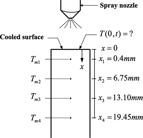
The main purpose of the present study is to use an analytical method to estimate the unknown surface heat flux and temperature on the hot surface of the test material during spray cooling. The present problem may be illustrated using a one-dimensional heat conduction problem. The physical geometry of the present problem is shown in Figure 1. The mathematical formulation, basic assumptions and experimental temperature data used in this study come from the works of Qiao and Chandra [1] and Cui et al. [3]. The surface heat flux and surface temperature on the hot surface of the test material are assumed to be unknown in the present study. These unknown values may be estimated provided that additional temperature measurement within the test material can be given. Thus, four thermocouples are used to obtain the experimental temperature data in order to investigate the effects of the measurement locations and the distance from the hot surface of the test material. The IHCP investigated here involve the estimates of the unknown surface heat flux and temperature from the transient temperature measurements at x = x_m. The governing differential equation, boundary conditions and initial condition are expressed as(1) $$k\frac{{\text{d}}^{2}T}{\text{d}{x}^2}=\mathit{\rho }c\frac{\mathit{\partial }T}{\mathit{\partial }t},0<x<L,0<t\le t_f$$(1) (2) $$T(L,t)=T_L(t),$$(2) (3) $$T(x_m,t)=T_m(t),$$(3) (4) $$T(0,t)=T_0(t),$$(4)

Figure 1. Physical geometry for temperature measurements of a hot plate during spray cooling.

and(5) $$T(x,0)=T_{\text{in}},$$(5)

where T is the temperature; t and x, respectively, denote time and space variables; k is the thermal conductivity of the test material; ρ is the density; c is the specific heat; L is the distance from the hot surface of the test material; T_L(t) is the given temperature measurement at x = L; x_m denotes the measurement location; T_in is the initial temperature; t_f denotes time that spray cooling is terminated; T_in(t) is the experimental temperature data at x = x_m. An appropriate polynomial function in each sub-time interval is applied to fit the experimental temperature data at each measurement location. T₀(t) is the unknown surface temperature on the hot surface and is obtained using the given temperature measurements at x = x_m and x = L.

3. Analytical method

In order to remove the time-dependent terms from the governing differential equation and boundary conditions, the method of the Laplace transform is employed. The Laplace transform of Equations (1)–(4) with respect to time in conjunction with the initial condition (5(5) $$T(x,0)=T_{\text{in}},$$(5) ) gives(6) $$\frac{{\text{d}}^2\tilde{T}}{\text{d}{\text{x}}^2}-\frac{s}{\mathit{\alpha }}\tilde{T}=-\frac{T_{\text{in}}}{\mathit{\alpha }},0<x<L$$(6) (7) $$\tilde{T}(L)={\tilde{T}}_L,\text{at}x=L$$(7)

and(8) $$\tilde{T}(x_m)={\tilde{T}}_m,\text{at}x=x_m$$(8)

where α = k/(ρc) is the thermal diffusivity of the test material; s is the Laplace transform parameter. Assume $\tilde{\mathit{\phi }}(x,s)$ is the Laplace transform of the function φ and is expressed as(9) $$\tilde{\mathit{\phi }}(x,s)={\int }_0^{\infty }{e}^{-st}\mathit{\phi }(x,t)\text{d}t.$$(9)

It is easy to obtain the solution of Equation (6) with the boundary conditions (7) and (8) as(10) $$\tilde{T}(x,s)=\left({\tilde{T}}_L-\frac{T_{\text{in}}}{s}\right)\frac{\text{sinh}\left[\sqrt{\frac{s}{a}}(x-x_m)\right]}{\text{sinh}\left[\sqrt{\frac{s}{a}}(L-x_m)\right]}+\left({\tilde{T}}_m-\frac{T_{\text{in}}}{s}\right)\frac{\text{sinh}\left[\sqrt{\frac{s}{a}}(L-x)\right]}{sinh\left[\sqrt{\frac{s}{a}}(L-x_m)\right]}+\frac{T_{\text{in}}}{s}.$$(10)

By the existence theorem of the Laplace transform, the function φ(x, t) is piecewise continuous in [0, ∞) if there exist a finite number of points_. The function φ(x, t) is continuous in each sub-time interval. It may be difficult to obtain an approximate polynomial function that can fit the experimental temperature measurements for the whole time domain under consideration. Thus, based on this existence theorem, the whole time domain may be divided into p sub-time intervals from the initial measurement time t₀. Assume the interface points between two adjacent sub-time intervals are τ₁, τ₂, …, τ_p−1. Thus, φ(x, t) can be expressed as φ(x, t) = φ₀(x, t)[U(t) − U(t − τ₁)] + φ₁(x, t)[U(t − τ₁) − U(t − τ₂)] + … + φ_p−1(x, t)U(t − τ_p−1). It can be proved by the second shifting theorem of the Laplace transform that the proposed method can be used to determine a solution for each sub-time interval. From [9,10], the estimated value of the unknown surface condition obtained by this method has good accuracy. This implies that obtained function q(0, t) is independent of the polynomial function of T_m(t) and T_L(t) out of an analysis sub-time interval. An approximate polynomial function with the least squares curve fitting method is used to fit the experimental temperature data throughout the whole time domain. The experimental temperature data T_m(t) and T_L(t) are approximated by an Nth degree polynomial function of time for each sub-time interval t_i ≤ t ≤ t_i+N (i = 1, 2, …, p − 1) and are written as(11) $$T_m(t)=\sum _{j=0}^N{C}_j{t}^j$$(11)

and(12) $$T_L(t)=\sum _{j=0}^N{E}_j{t}^j,$$(12)

where the coefficients C_j and E_j are obtained based on the corresponding curve fitting temperatures.

The Laplace transform of Equations (11(6) $$\frac{{\text{d}}^2\tilde{T}}{\text{d}{\text{x}}^2}-\frac{s}{\mathit{\alpha }}\tilde{T}=-\frac{T_{\text{in}}}{\mathit{\alpha }},0<x<L$$(6) ) and (12(7) $$\tilde{T}(L)={\tilde{T}}_L,\text{at}x=L$$(7) ) with respect to time in each sub-time interval is(13) $${\tilde{T}}_m(s)=\frac{C_0}{s}+\sum _{n=1}^N{C}_n\frac{n!}{s^{n+1}}$$(13)

and(14) $${\tilde{T}}_L(s)=\frac{E_0}{s}+\sum _{n=1}^N{E}_n\frac{n!}{s^{n+1}}.$$(14)

The unknown surface heat flux on the hot surface q(0, t) can be expressed as(15) $$q(0,t)=k\frac{\mathit{\partial }}{\mathit{\partial }x}T(0,t).$$(15)

Thus, the unknown surface temperature and heat flux on the hot surface T(0, t) and q(0, t) in each sub-time interval are obtained from Equation (10) as(16) $$\begin{array}{cc}T(0,t)\hfill & =L^{-1}\left[\tilde{T}(x,s)\right]\hfill \\ \hfill & =L^{-1}\left\{\frac{\left({\tilde{T}}_m-\frac{T_{\text{in}}}{s}\right)\text{sinh}\left(\sqrt{\frac{s}{a}}L\right)-\left({\tilde{T}}_L-\frac{T_{\text{in}}}{s}\right)\text{sinh}\left(\sqrt{\frac{s}{a}}{x}_m\right)}{\text{sinh}\left[\sqrt{\frac{s}{a}}(L-x_m)\right]}+\frac{T_{\text{in}}}{s}\right\}\hfill \end{array}$$(16)

and(17) $$\begin{array}{cc}q(0,t)\hfill & =k{L}^{-1}\left[\frac{\mathit{\partial }}{\mathit{\partial }x}T(0,s)\right]\hfill \\ \hfill & =k{L}^{-1}\left\{\sqrt{\frac{s}{a}}\times \frac{\left({\tilde{T}}_L-\frac{T_{\text{in}}}{s}\right)\text{cosh}\left(\sqrt{\frac{s}{a}}{x}_m\right)-\left({\tilde{T}}_m-\frac{T_{\text{in}}}{s}\right)\text{cosh}\left(\sqrt{\frac{s}{a}}L\right)}{\text{sinh}\left[\sqrt{\frac{s}{a}}(L-x_m)\right]}\right\}\hfill \end{array}$$(17)

where L⁻¹ denotes the inverse of the Laplace transform.

Many computing methods can be applied to perform the inverse of the Laplace transform. The numerical inversion of the Laplace transform proposed by [11] is based on a Fourier series expansion. We established a sub-routine about the inverse Laplace transform and the main programme in conjunction with the sub-routines given by [11] to solve all kinds of transient heat conduction problems, as shown in [9, 10, 12, 13]. It is seen in [12, 13] that the results obtained are close to the exact solution. The resulting estimates of T(0, t) and q(0, t) given by [10] are also in good agreement with the exact results for the whole time domain, even in a short time domain of 0 < t ≤ 0.2 s. Therefore, the present results are accurate. This implies that the numerical inversion of the Laplace transform [11] has good accuracy. The details of the numerical inversion of Laplace transform can be found in [11, 12]. To avoid duplication, they are not reiterated in this manuscript. Thus, this study applies the numerical inversion of the Laplace transform [11] in conjunction with Equations (5(5) $$T(x,0)=T_{\text{in}},$$(5) ), (13(8) $$\tilde{T}(x_m)={\tilde{T}}_m,\text{at}x=x_m$$(8) ) and (14(14) $${\tilde{T}}_L(s)=\frac{E_0}{s}+\sum _{n=1}^N{E}_n\frac{n!}{s^{n+1}}.$$(14) ) to perform the inverse of Equations (16) and (17). Obviously, the present inverse scheme is simpler than that proposed by [9]. In addition, the functional form of the unknown surface temperature need not be assumed in advance before performing the inverse calculation so that the proposed method does not require any iteration and initial guess.

4. Results and discussion

In order to demonstrate the accuracy and reliability of the present scheme, two experimental examples given by [1,3] and one analytical example are illustrated. Thus, the comparison between the present results, exact results and those given by [1,3,9] is made.

4.1. Example 1

A schematic diagram of the apparatus used for spraying cooling experiments with pure water is shown in Figure 1. The detailed experimental processes can refer to [1]. Qiao and Chandra [1] and Chen and Lee [9], respectively, applied the sequential function specification method [5] and the hybrid inverse method of the Laplace transform and the finite difference method to estimate the unknown surface heat flux q(0, t) and temperature T(0, t) during spray quenching. Chen and Lee [9] divided the whole time domain into two sub-time intervals. Then, they applied an Nth degree approximate polynomial function (N = 5–9) in conjunction with the least squares curve fitting method to fit the experimental temperature data in each sub-time interval for four different measurement locations. The thermophysical quantities in Example 1 are given as ρ = 8933 kg/m³, k = 385.1 W/(m °C), c = 412.66 J/(kg °C) and T_in = 240 °C.[9] The initial measurement time t₀ and the measurement time step ∆t_e are t₀ = ∆t_e = 5 s for this example. This implies that the total number of discrete measurement times is equal to 20. The main purpose of the present study is to apply the experimental temperature data given in [1] to investigate the accuracy of the present estimated results. Thus, the comparison of the unknown surface temperature and heat flux between the present results and those given in [1,9] is made.

Qiao and Chandra [1] applied the K-type (chromel–alumel) thermocouple with a diameter of 0.5 mm to measure the temperature of the test cylinder at four different measurement locations x₁, x₂, x₃ and x₄. These four thermocouples are inserted into holes drilled 6.35 mm apart along the axis of the copper cylinder. However, the first thermocouple is positioned 0.4 mm below the cold surface of the test cylinder. On the other hand, x₁, x₂, x₃ and x₄ are given as x₁ = 0.4 mm, x₂ = 6.75 mm, x₃ = 13.1 mm and x₄ = 19.45 mm. The measured temperature is continuously recorded using a digital data acquisition system. The experimental temperature data at the four different measurement locations, a spray mass flux m₁ = 0.5 kg/(m² s) and a mean droplet impact velocity U_m = 20 m/s have been shown in Figure 4 of [1] and Figure 2 of [9].

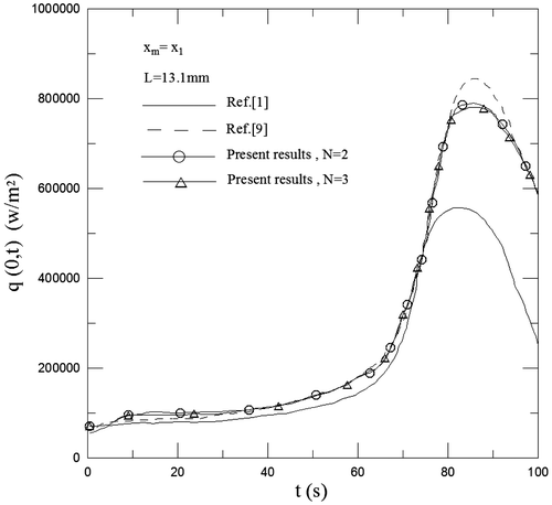
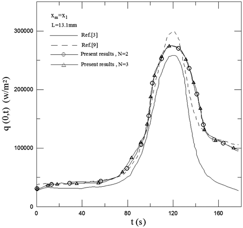
In order to investigate the effects of the distance from the hot surface of the test material and the degree of approximate polynomial function, quadratic (N = 2) and cubic degree polynomial functions (N = 3) are selected to approximate the experimental temperature data in each sub-time interval for four measurement locations. Figure 2 shows the comparison of T(0, t) between the present results and those given in [1,9] for x_m = x₁, L = 13.1 mm and various N values. The extrapolation of the approximate cubic polynomial function with the least squares curve fitting method is used to determine the unknown surface heat flux for 0 ≤ t ≤ t₀. The comparison of q(0, t) between the present results and those given in [1,9] is shown in Figure 3 for x_m = x₁, L = 13.1 mm and various N values. However, the present results of T(0, t) and q(0, t) for L = 19.45 mm are in good agreement with those for L = 13.1 mm under the same conditions. Thus, the comparison of T(0, t) and q(0, t) between the present results and those given in [1,9] for L = 19.45 mm will not be shown in this paper. In Figure 2, the difference of T(0, t) between the results obtained from N = 2 and 3 is small. An interesting finding is that the present results of T(0, t) agree well with those obtained by [1,9]. The present results of q(0, t) are also consistent with those obtained by [9] when 0 < t ≤ 110 s except for 70 s < t < 90 s. The maximum deviation of q(0, t) between them occurs around at t = 85 s. Their deviation at t = 85 s is about 8%. This deviation may come from that q(0, t) has a peak value and steep change around at t = 85 s. Chen and Lee [9] divided the whole time domain into two sub-time intervals for the experimental temperature data and selected the quadratic polynomial guess function of time to approximate the unknown surface temperature data in each analysis sub-time interval. In addition, a higher degree of approximate polynomial function (N = 5–9) is applied to fit the experimental temperature data for four different measurement locations. Obviously, this method is different from the present method. The present results of q(0, t) only agree with those obtained by [1] for 0 < t ≤ 75 s. The difference of q(0, t) between them may become larger for 75 s < t ≤ 110 s. It is also observed from Figure 3 that the present results of q(0, t) are lower than those given by [9] when 75 s < t < 90 s and higher than those obtained by [1] when 75 s < t ≤ 110 s. This implies that the estimated results of q(0, t) obtained by [1] may be underestimated for larger values of time.

Figure 2. A comparison of T(0, t) with x_m = x₁, L = 13.1 mm and various N values.

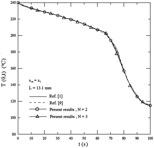
Figure 3. A comparison of q(0, t) with x_m = x₁, L = 13.1 mm and various N values.

In order to investigate the effect of the measurement location on the present results, Table 1 shows the comparison of T(0, t) and q(0, t) for L = 13.1 mm, N = 3 and various x_m values. It is observed from Table 1 that the results of T(0, t) and q(0, t) obtained from x_m = x₂ agree well with those from x_m = x₁. The above results indicate that, in order to obtain a good estimation, it is not always recommended to choose the measurement location as close as possible to the surface of the unknown boundary condition. The present results of q(0, t) do not exhibit oscillations when the experimental temperature data are used.

Table 1. A comparison of the present estimates with N = 3, L = x₃ and various x_m values.

t	Present estimates				xm = x2
	xm = x1		xm = x2		Ref. [1]		Ref. [9]
	T(0, t)	q(0, t)	T(0, t)	q(0, t)	T(0, t)	q(0, t)	T(0, t)	q(0, t)
0	240.0	70,336	240.0	71,352	240.0	69,854	240.0	70,528
10	233.3	96,034	233.2	97,227	232.9	78,223	233.0	95,922
20	228.6	96,923	229.0	87,042	228.8	78,223	229.1	86,356
30	233.3	95,474	224.8	87,772	224.6	83,640	224.6	89,392
40	219.4	116,547	219.6	109,764	219.6	95,341	219.2	111,885
50	213.7	146,984	213.4	155,615	213.8	113,543	213.4	146,133
60	207.3	176,177	206.4	185,114	206.7	147,996	206.8	188,362
70	195.0	310,449	193.8	311,922	195.1	288,407	193.4	301,843
80	156.8	768,100	157.1	740,779	155.7	565,330	158.0	754,317
90	126.8	746,470	127.0	740,841	124.6	507,259	125.6	793,934
100	115.2	611,389	113.7	602,053	115.1	255,255	114.1	615,731
110	113.5	447,043	112.0	487,640	113.0	136,078	113.2	450,878

4.2. Example 2

The problem with spray cooling proposed by [3] is also illustrated in order to investigate the accuracy of the present inverse scheme further. A schematic diagram of the apparatus built to estimate the unknown surface temperature and surface heat flux during spray cooling has been shown in Figure 1 of [3]. This instrument is a modified version of one designed by [1]. The main components of this system are a water delivery system, a spray nozzle, a heated copper test surface, a data acquisition and control system to record the experimental temperature data at four different measurement locations. However, the governing differential equation, boundary conditions, initial condition and some thermophysical quantities are not shown in their work [3]. In order to compare with the estimated results of the unknown surface temperature and heat flux given by [3,9], the material of the heated test cylinder is assumed to be brass. Thus, the thermophysical quantities of this example are ρ = 8530 kg/m³, k = 144.4 W/(m °C), c = 412.0 J/(kg °C) and T_in = 240 °C; t₀ and ∆t_e are also t₀ = ∆t_e = 5 s for Example 2. This implies that the total number of discrete measurement times is equal to 34.

Cui et al. [3] also applied the K-type (chromel–alumel) thermocouple with a diameter of 0.5 mm to measure the temperature of the test cylinder at four different measurement locations x₁, x₂, x₃ and x₄. These four different measurement locations are the same as those given in [1], i.e. x₁ = 0.4 mm, x₂ = 6.75 mm, x₃ = 13.1 mm and x₄ = 19.45 mm. The experimental temperature data at x = x₁, x₂, x₃ and x₄ are continuously recorded using a digital data acquisition system. These temperature data have been shown in Figure 2 of [3] and Figure 9 of [9]. Chen and Lee [9] still divided the whole time domain into two sub-time intervals. Later, they applied an Nth degree approximate polynomial function (N = 6–8) in conjunction with the least squares fitting method to fit these temperature data in each sub-time interval.

The present study applies the experimental temperature data [3] to determine the unknown surface temperature and heat flux during the spraying cooling. Cui et al. [3] also applied the sequential function specification method to estimate the unknown surface heat flux and temperature. In order to validate the accuracy of the present inverse scheme, the comparison of the unknown surface temperature and heat flux between the present results and those given by [3,9] is made. Quadratic (N = 2) and cubic (N = 3) polynomial functions are selected to approximate the experimental temperature data in each sub-time interval for four different measurement locations. These results show that the deviation of the results obtained with L = 13.1 and 19.45 mm is small. The results obtained from x_m = x₁ are also in good agreement with those from x_m = x₂. The similar conclusion can be found as that yield in Example 1. Thus, these results will not be shown in this paper. This implies that the present analytical method may not be very sensitive to the distance from the hot surface of the test material and the measurement location.

Figures 4 and 5, respectively, show the comparison of T(0, t) and q(0, t) between the present results and those obtained by [3,9] for L = 13.1 mm, x_m = x₁ and various N values. It is found from these two figures that the results of T(0, t) and q(0, t) obtained from N = 2 agree with those from N = 3. Like results of Example 1, Figure 4 shows that the present results of T(0, t) agree well with those obtained by [3,9] for the whole time considered. The present results of q(0, t) are also consistent with those obtained by [9] when 0 < t ≤ 180 s except for 110 s < t < 130 s. The maximum deviation of q(0, t) between them occurs around at t = 120 s. Their deviation at t = 120 s is about 11%. It is found from Figure 5 that the unknown surface heat flux q(0, t) also has a peak value and an abrupt change around at t = 120 s. This phenomenon is similar to that shown in Example 1. However, the present results of q(0, t) are higher than those obtained by [3] when 0 < t ≤ 180 s and can deviate slightly from their estimated results when 0 < t ≤ 100 s. Their deviation may become larger for 100 s < t ≤ 180 s.

Figure 4. A comparison of T(0, t) with various N values.

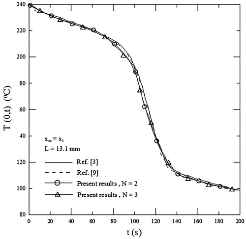
Figure 5. A comparison of q(0, t) with various N values.

In accordance with the results in Examples 1 and 2, a larger deviation of q(0, t) between the present results and those given by [9] may come from the number of the sub-time interval, the assumption of the quadratic polynomial guess function and the degree of approximate polynomial function.

Qiao and Chandra [1] and Cui et al. [3] applied the sequential function specification method in conjunction with the experimental temperature data to predict the unknown surface heat flux. Their works are useful for validating the accuracy and reliability of an inverse heat conduction scheme. It is found in [5] that the sequential function specification method can be sensitive to the ‘thermocouples’ locations, number of future times, measurement errors and time step. In addition, the small dimensionless time should be based on the distance from the heated surface to the thermocouple nearest the heated surface.

4.3. Example 3

This analytical example proposed by [6, 12] is illustrated to investigate the reliability of the present inverse scheme further. The physical quantities in this example are assumed to be L = 1 m, α = 1 m²/s, T₀(t) = a₀, T_L(t) = a_L and T_in = 0 °C.(18) $$T(x,t)=a_0(1-x)+a_{L}x+\left[-2\sum _{m=1}^{\infty }{e}^{-{\mathit{\beta }}_m^{2}t}[a_0-a_{L}cos({\mathit{\beta }}_m)]\frac{sin({\mathit{\beta }}_{m}x)}{{\mathit{\beta }}_m}\right]$$(18)

where β_m is defined as β_m = mπ.

In order to simulate the experimental temperature data T_mea, the exact data T_exa can be modified by adding a small random error. Thus, this temperature measurement T_mea is expressed as(19) $$T(x_m,t_r)=T_{\text{exa}}(x_m,t_r)(1+\mathit{\omega }),\text{for}{t}_0\le t_r\text{and}r=0,1,\dots ,M-1,$$(19)

where ω denotes the error limit of the thermocouple and is assumed to be |ω| ≤ 5%.

The initial measurement time t₀ and measurement time step ∆t_e are 0.1 and 0.05 s, respectively. The total number of discrete measurement times is equal to 11. In order to obtain a good estimate, it is suggested that the choice of N is as close as possible to $2\sqrt{M}-1$. Figure 6 shows the simulated temperature data for a₀ = 1000 °C, a_L = 0 °C, ω = 5% and various x_m values. An Nth degree approximate polynomial function in combination with the least squares fitting method is applied to fit the experimental temperature data in each sub-time interval for each specific measurement location. Figure 7 shows a comparison of T(0, t) for a₀ = 1000 °C, a_L = 0 °C, x_m = 0.5 m and various values of ω and N. A comparison of q(0, t) is shown in Figure 8 for a₀ = 1000 °C, a_L = 0 °C, x_m = 0.5 m and various values of ω and N. The extrapolation method is applied to determine the present estimates in a short time range of 0 < t < 0.1 s. It is found from Figures 7 and 8 that the estimated results of T(0, t) and q(0, t) obtained agree well with the exact result for N = 2, 3 and 6 even with ω = 10%. The present estimates of q(0, t) are in good agreement with the exact solution for t ≥ 1 s and deviate slightly from the exact solution in a short time range of 0 < t < 0.1 s. Figures 7 and 8 show the estimated values of T(0, t) and q(0, t) obtained do not exhibit severe oscillation for ω = 0, 5 and 10%, and are not very sensitive to the Nth-order polynomial function for 2 ≤ N ≤ 6. Thus, this inverse scheme has good stability and accuracy. However, it is found in [8] that the front surface heat flux deviates slightly from the exact solution and exhibits oscillations in a short time when the sensor noise is incorporated into the back surface temperature measurement. An interesting finding is that the present estimates are not always improved with an increase in the value of N. A comparison of the present estimates is shown in Table 2 with a₀ = 1000 °C, a_L = 0 °C, N = 3, ω = 5% and various x_m values. The results show that the present estimates of T(0, t) and q(0, t) do not exhibit severe oscillation phenomenon and are in good agreement with the exact result for ω = 5% and x_m = 0.5 and 0.85 m. This implies that the effect of the measurement location on the present estimates is small. In order to validate the effect of N and x_m values, the problem with a₀ = a_L = 1 °C is also illustrated. A comparison of the present estimates is shown in Table 3 with a₀ = a_L = 1 °C, ω = 5% and various values of N and x_m. It is found that the present estimates of T(0, t) still agree with the exact results for ω = 5%, x_m = 0.5 m and N = 3 and 6. It is worth mentioning that the present estimates of q(0, t) using N = 3 is closer to the exact solution than those using N = 6. The present estimates for x_m = 0.1 m can also be more accurate than those for x_m = 0.5 m. However, the deviation between them is small. Accordingly, the results in this example further indicate that the present scheme may not be very sensitive to the measurement location. It can be found in [6] that a suitable degree approximate polynomial function falls in the range of 5–7. This difference between the present results and those obtained by [6] may result from the assumption of temperature measurements with half polynomial series of time, the use of sub-time intervals, etc.

Figure 6. Simulated temperature data with $\mathit{\omega }$ = 5% at various x_m values.

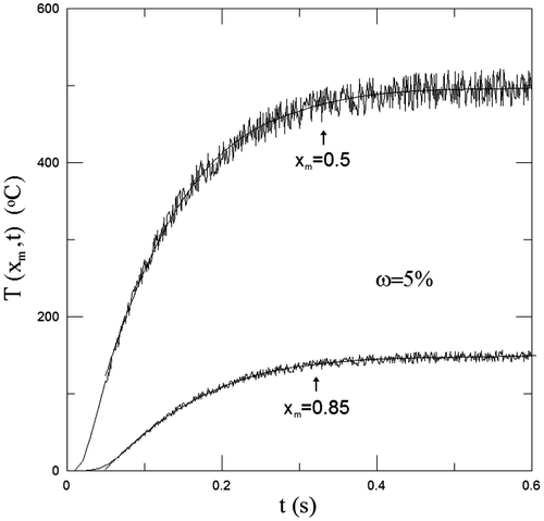
Figure 7. A comparison of T(0, t) with a₀ = 1000 °C, a_L = 0 °C, x_m = 0.5 m and various values of $\mathit{\omega }$ and N.

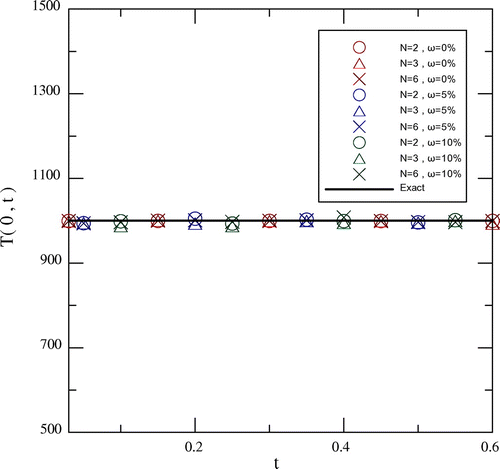
Figure 8. A comparison of q(0, t) with a₀ = 1000 °C, a_L = 0 °C, x_m = 0.5 m and various values of $\mathit{\omega }$ and N.

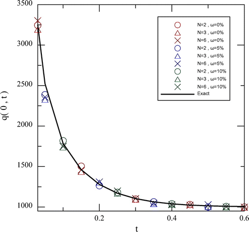
Table 2. A comparison of the present estimates with a₀ = 1000 °C, a_L = 0 °C, N = 3, $\mathit{\omega }$ = 5% and various x_m values.

t	Texa(0, t)	T(0, t)		qexa(0, t)	q(0, t)
		xm = 0.5	xm = 0.85		xm = 0.5	xm = 0.85
0.05	1000	999.736	994.636	2523.133	2504.738	2372.202
0.1	1000	999.472	989.271	1784.286	1818.581	1829.885
0.15	1000	998.580	1007.495	1460.439	1447.891	1535.834
0.2	1000	995.717	1000.328	1278.567	1274.606	1278.099
0.25	1000	998.357	995.743	1169.713	1180.664	1152.582
0.3	1000	998.132	1001.206	1103.561	1099.754	1139.633
0.35	1000	997.478	998.576	1063.217	1060.867	1061.402
0.4	1000	998.081	997.443	1038.593	1039.565	1032.915
0.45	1000	998.030	998.787	1023.561	1021.153	1030.843
0.5	1000	997.881	998.131	1014.384	1012.309	1012.426
0.55	1000	998.019	997.873	1008.781	1007.457	1005.945
0.6	1000	998.007	998.180	1005.361	1003.268	1005.475

Table 3. A comparison of the present estimates with a₀ = a_L = 1 °C, $\mathit{\omega }$ = 5% and various values of N and x_m.

t	Texa(0, t)	T(0, t)			qexa(0, t)	q(0, t)
		xm = 0.1	xm = 0.5	xm = 0.5		xm = 0.1	xm = 0.5	xm = 0.5
		N = 3	N = 3	N = 6		N = 3	N = 3	N = 6
0.05	1	1.000	1.012	1.002	2.489	2.194	2.211	1.910
0.1	1	1.000	1.024	1.003	1.491	1.444	1.568	1.406
0.15	1	1.006	1.032	0.992	0.910	0.903	0.878	0.860
0.2	1	1.007	1.001	0.996	0.556	0.547	0.543	0.564
0.25	1	0.999	0.995	1.008	0.339	0.313	0.360	0.393
0.3	1	0.995	1.000	1.018	0.207	0.193	0.192	0.271
0.35	1	0.994	1.033	1.018	0.126	0.118	0.133	0.165
0.4	1	0.997	1.014	1.015	0.077	0.074	0.078	0.077
0.45	1	1.000	1.007	1.007	0.047	0.040	0.040	0.026
0.5	1	1.001	1.006	1.005	0.029	0.025	0.030	0.033
0.55	1	0.999	0.984	1.022	0.018	0.016	0.019	0.012
0.6	1	0.994	1.000	1.002	0.011	0.008	0.009	0.007

6. Conclusions

This study proposes an analytical inverse scheme combined with the Laplace transform method, the sequential-in-time concept and experimental temperature data within the test material to estimate the unknown surface temperature and heat flux on a hot surface during spray cooling. Experimental and analytical examples show that the obtained estimates of the unknown surface temperature T(0, t) agrees well with the exact results and those given by [1,3,9] for the whole time domain considered. The deviation of the unknown surface heat flux q(0, t) between the present estimates and those given by [9] is small. However, the obtained results of q(0, t) can slightly deviate from those given by [1,3] in the early time. Later, their deviation may become larger in the late time. The proposed method is not very sensitive to the measurement location provided that the suitable value of t₀ can be selected. Importantly, this method does not require any iteration and initial guess. The resulting estimates do not exhibit serious oscillation. An interesting finding is that the present estimates are not necessarily improved with an increase in the value of N.

Nomenclature
c	=	specific heat, J/kg °C
k	=	thermal conductivity, W/m °C
L	=	distance from the hot surface of the test material, m
M	=	number of discrete measurement times in each sub-time interval
m1	=	spray mass flux, kg/m2 s
N	=	degree of polynomial function
P	=	number of sub-time intervals
s	=	Laplace transform parameter
T	=	temperature, °C
$\tilde{T}$	=	temperature in the transform domain
Tin	=	initial temperature, °C
TL(t)	=	given temperature measurement at x = L, °C
Tm(t)	=	experimental temperature data at x = xm, °C
T0(t)	=	unknown surface temperature on the hot surface, °C
t	=	time, s
tf	=	final time, s
Um	=	mean droplet impact velocity, m/s
x	=	spatial coordinate, m
xm	=	location of the thermocouple

Greeks symbols
α	=	thermal diffusivity, m2/s
ρ	=	density, kg/m3

Disclosure statement

No potential conflict of interest was reported by the authors.

References

- Qiao YM, Chandra S. Spray cooling enhancement by addition of a surfactant. J. Heat Transfer. 1998;120:92–98.10.1115/1.2830070
- Jia W, Qiu HH. Experimental investigation of droplet dynamics and heat transfer in spray cooling. Exp. Therm. Fluid Sci. 2003;27:829–838.10.1016/S0894-1777(03)00015-3
- Cui Q, Chandra S, McCahan S. The effect of dissolving salts in water sprays used for quenching a hot surface: part 2 – spray cooling. J. Heat Transfer. 2003;125:333–338.10.1115/1.1532011
- Hsieh SS, Fan TC, Tsai HH. Spray cooling characteristics of water and R-134a. Part II: transient cooling. Int. J. Heat Mass Transfer. 2004;47:5713–5724.10.1016/j.ijheatmasstransfer.2004.07.023
- Kurpisz K, Nowak AJ. Inverse thermal problems. Southampton: Computational Mechanics Publications; 1995.
- Monde M, Arima H, Mitsutake Y. Estimation of surface temperature and heat flux using inverse solution for one-dimensional heat conduction. J. Heat Transfer. 2003;125:213–223.10.1115/1.1560147
- Woodfield PL, Monde M, Mitsutake Y. Implementation of an analytical two-dimensional inverse heat conduction technique to practical problems. Int. J. Heat Mass Transfer. 2006;49:187–197.10.1016/j.ijheatmasstransfer.2005.06.035
- Feng ZC, Chen JK, Zhang Y. Temperature and heat flux estimation from sampled transient sensor measurements. Int. J. Therm. Sci. 2010;49:2385–2390.10.1016/j.ijthermalsci.2010.08.004
- Chen HT, Lee HC. Estimation of spray cooling characteristics on a hot surface using the hybrid inverse scheme. Int. J. Heat Mass Transfer. 2007;50:2503–2513.10.1016/j.ijheatmasstransfer.2006.12.021
- Chen HT, Lin JH, Xu XJ. Analytical estimates of surface conditions in laser surface heating process with experimental data. Int. J. Heat Mass Transfer. 2013;67:936–943.10.1016/j.ijheatmasstransfer.2013.08.093
- Honig G, Hirdes U. A method for the numerical inversion of Laplace transforms. J. Comput. Appl. Math. 1984;10:113–132.10.1016/0377-0427(84)90075-X
- Chen HT, Chen TM, Chen CK. Hybrid Laplace transform/finite element method for one-dimensional transient heat conduction problems. Comput. Methods Appl. Mech. Eng. 1987;63:83–95.
- Chen HT, Chang SM. Application of the hybrid method to inverse heat conduction problems. Int. J. Heat Mass Transfer. 1990;33:621–628.10.1016/0017-9310(90)90161-M