Reconstruction of multiplicative space- and time-dependent sources

Abstract

This paper presents a numerical regularization approach to the simultaneous determination of multiplicative space- and time-dependent source functions in a nonlinear inverse heat conduction problem with homogeneous Neumann boundary conditions together with specified interior and final time temperature measurements. Under these conditions a unique solution is known to exist. However, the inverse problem is still ill-posed since small errors in the input interior temperature data cause large errors in the output heat source solution. For the numerical discretisation, the boundary element method combined with a regularized nonlinear optimization are utilized. Results obtained from several numerical tests are provided in order to illustrate the efficiency of the adopted computational methodology.

Keywords:

• Inverse source problem
• boundary element method
• nonlinear optimization
• regularization

AMS Subject Classifications:

• 65M32
• 65M38

1. Introduction

Solving inverse source problems for the parabolic heat equation has been the point of interest for many works, see [1–7] to mention only a few, due to their ever increasing applications in problems related to pollution, unknown heat source generation or control of oil wells and their production rates. Almost all the previous studies generally assumed that the unknown heat source is independent of one or more of the independent variables in order to ensure the uniqueness of solution. On the other hand, only a few studied looked at the general case,[8] but the classes of functions in which the source is to lay were further restricted with constraints which are difficult to satisfy in practice (both experimental and computational). Recently, the authors investigated the reconstruction of an additive source of the form $\mathit{\varphi }(t)+\mathit{\psi }(x)$, see [9]. In this work, we extend the investigation to include the reconstruction of a multiplicative source of the form r(t)s(x), in which both r(t) and s(x) are unknown functions. In contrast to the previously investigated linear reconstruction of the additive source, this new inverse source problem formulation is more difficult to solve because it now becomes nonlinear. Moreover, its ill-posednes with respect to small errors in the input data being blown up in the output source solution adds even further difficulty.

The plan of the paper is as follows. In Section 2, we give the mathematical formulation of the inverse multiplicative source problem and state its unique solvability. In Section 3, we describe the numerical discretisation of the problem based on the boundary element method (BEM), whilst in Section 4 we introduce the method for obtaining the solution based on a nonlinear least-squares minimization. Section 5 presents and discusses numerical results and illustrates the need for employing regularization in order to stabilise the solution. Finally, Section 6 presents the conclusions of the paper.

2. Mathematical formulation

Let $L>0$ and $T>0$ be fixed numbers and denote by $D_T:=\{(x,t)|0<x<L,0<t<T\}=(0,L)\times (0,T)$. Consider the following inverse initial-boundary value problem of finding the temperature u(x, t) and the multiplicatively separable source function $F(x,t):=r(t)s(x)$ which satisfy the equation(2.1) $$\begin{array}{c}\hfill {\displaystyle \frac{\mathit{\partial }u}{\mathit{\partial }t}}(x,t)={\displaystyle \frac{{\mathit{\partial }}^{2}u}{\mathit{\partial }{x}^2}}(x,t)+r(t)s(x),(x,t)\in D_T,\end{array}$$(2.1)

subject to the initial condition(2.2) $$\begin{array}{c}\hfill u(x,0)=\mathit{\phi }(x),x\in [0,L],\end{array}$$(2.2)

the homogeneous Neumann boundary conditions(2.3) $$\begin{array}{c}\hfill {\displaystyle \frac{\mathit{\partial }u}{\mathit{\partial }x}}(0,t)={\displaystyle \frac{\mathit{\partial }u}{\mathit{\partial }x}}(L,t)=0,t\in [0,T],\end{array}$$(2.3)

and the additional temperature measurement(2.4) $$\begin{array}{c}\hfill u(X_0,t)=\mathit{\beta }(t),t\in [0,T],\end{array}$$(2.4)

at a fixed sensor location $X_0\in (0,L)$, and(2.5) $$\begin{array}{c}\hfill u(x,T)=\mathit{\mu }(x),x\in [0,L],\end{array}$$(2.5)

at the ‘upper-base’ final time $t=T$. Conditions (2.3(2.3) $$\begin{array}{c}\hfill {\displaystyle \frac{\mathit{\partial }u}{\mathit{\partial }x}}(0,t)={\displaystyle \frac{\mathit{\partial }u}{\mathit{\partial }x}}(L,t)=0,t\in [0,T],\end{array}$$(2.3) ) express that the ends $\{0,L\}$ of the finite slab (0, L) are insulated. In order to avoid trivial non-uniqueness represented by the identity $r(t)s(x)=\frac{r(t)}{c}·cs(x)$, with c arbitrary non-zero constant, we impose a fixing condition, say(2.6) $$\begin{array}{c}\hfill s(X_0)=\mathit{\alpha }.\end{array}$$(2.6)

In the above setting, the functions $\mathit{\phi },\mathit{\beta },\mathit{\mu }$ and the constant $\mathit{\alpha }$ are given, whilst the functions $r(t),s(x)$ and u(x, t) are unknowns. One can remark that the specified interior and the final time temperature measurements (2.4(2.4) $$\begin{array}{c}\hfill u(X_0,t)=\mathit{\beta }(t),t\in [0,T],\end{array}$$(2.4) ) and (2.5(2.5) $$\begin{array}{c}\hfill u(x,T)=\mathit{\mu }(x),x\in [0,L],\end{array}$$(2.5) ) are time- and space-dependent functions $\mathit{\beta }(t)$ and $\mathit{\mu }(x)$ and, in principle, they are meant to supply the missing information to identify the time- and space-dependent components r(t) and s(x), respectively. However, because of the nonlinearity represented by the product r(t)s(x) we cannot decouple the system of Equations (2.1(2.1) $$\begin{array}{c}\hfill {\displaystyle \frac{\mathit{\partial }u}{\mathit{\partial }t}}(x,t)={\displaystyle \frac{{\mathit{\partial }}^{2}u}{\mathit{\partial }{x}^2}}(x,t)+r(t)s(x),(x,t)\in D_T,\end{array}$$(2.1) )–(2.6(2.6) $$\begin{array}{c}\hfill s(X_0)=\mathit{\alpha }.\end{array}$$(2.6) ) and identify separately r(t) and s(x) from (2.4(2.4) $$\begin{array}{c}\hfill u(X_0,t)=\mathit{\beta }(t),t\in [0,T],\end{array}$$(2.4) ) and (2.5(2.5) $$\begin{array}{c}\hfill u(x,T)=\mathit{\mu }(x),x\in [0,L],\end{array}$$(2.5) ), respectively.

We further assume that the conditions (2.2(2.2) $$\begin{array}{c}\hfill u(x,0)=\mathit{\phi }(x),x\in [0,L],\end{array}$$(2.2) )–(2.5(2.5) $$\begin{array}{c}\hfill u(x,T)=\mathit{\mu }(x),x\in [0,L],\end{array}$$(2.5) ) are consistent, i.e. the following compatibility conditions are satisfied:(2.7) $$\begin{array}{c}\hfill {\mathit{\phi }}^{\prime }(0)={\mathit{\phi }}^{\prime }(L)={\mathit{\mu }}^{\prime }(0)={\mathit{\mu }}^{\prime }(L)=0,\mathit{\beta }(0)=\mathit{\phi }(X_0),\mathit{\beta }(T)=\mathit{\mu }(X_0).\end{array}$$(2.7)

The unique solvability, i.e. existence and uniqueness of the solution of the inverse problem (2.1(2.1) $$\begin{array}{c}\hfill {\displaystyle \frac{\mathit{\partial }u}{\mathit{\partial }t}}(x,t)={\displaystyle \frac{{\mathit{\partial }}^{2}u}{\mathit{\partial }{x}^2}}(x,t)+r(t)s(x),(x,t)\in D_T,\end{array}$$(2.1) )–(2.6(2.6) $$\begin{array}{c}\hfill s(X_0)=\mathit{\alpha }.\end{array}$$(2.6) ), was established in [10]. With some slight corrections, this theorem reads as follows.

Theorem 1:

Suppose that $\mathit{\phi }(x)\in H^4(0,L),\mathit{\mu }(x)\in H^4(0,L)$ and $\mathit{\beta }(t)\in H^2(0,T)$ satisfy (2.7(2.7) $$\begin{array}{c}\hfill {\mathit{\phi }}^{\prime }(0)={\mathit{\phi }}^{\prime }(L)={\mathit{\mu }}^{\prime }(0)={\mathit{\mu }}^{\prime }(L)=0,\mathit{\beta }(0)=\mathit{\phi }(X_0),\mathit{\beta }(T)=\mathit{\mu }(X_0).\end{array}$$(2.7) ) and that $\mathit{\alpha }\ne 0$. Also, assume that:

(i)	$d:={\mathit{\beta }}^{\prime }(0)-{\mathit{\phi }}^{″}(X_0)\ne 0$,    $m:={\displaystyle \frac{{\mathit{\beta }}^{\prime }(T)-{\mathit{\mu }}^{″}(X_0)}{d}}\ne 0$,
(ii)	${\mathit{\phi }}^{″\prime }(0)={\mathit{\phi }}^{″\prime }(L)={\mathit{\mu }}^{″\prime }(0)={\mathit{\mu }}^{″\prime }(L)=0$,
(iii)	${\mathit{\lambda }}_1<1,4{\mathit{\lambda }}_2{\mathit{\lambda }}_3-{(1-{\mathit{\lambda }}_1)}^2\le 0,{\mathit{\lambda }}_4<1$,

where

${\mathit{\lambda }}_1:={\displaystyle \frac{2}{m^2{d}^2}}max\left\{d^2+{\displaystyle \frac{4L^2{\Vert {\mathit{\beta }}^{″}\Vert }^2}{{\mathit{\pi }}^2}}{,4L\Vert \mathit{\theta }\Vert }^2+L{m}^2{\Vert {\mathit{\phi }}^{″\prime }\Vert }^2\right\}$,

${\mathit{\lambda }}_2:={\displaystyle \frac{2}{d^2}}max\left\{{\displaystyle \frac{4L^6}{{\mathit{\pi }}^4{m}^4}},1\right\},{\mathit{\lambda }}_3:={\displaystyle \frac{2\Vert {\mathit{\theta }}^{\prime }{\Vert }^2}{m^2}}+{\displaystyle \frac{4\Vert {\mathit{\beta }}^{″}{\Vert }^2}{d^2}}\left({\displaystyle \frac{{2\Vert \mathit{\theta }\Vert }^2}{m^2}}+{\Vert {\mathit{\phi }}^{″\prime }\Vert }^2\right)$,

${\mathit{\lambda }}_4:={\displaystyle \frac{1}{m^2{d}^2}}max\left\{d^2+2L^3{z}_0+4L^2\Vert {\mathit{\beta }}^{″}{\Vert }^2,4L^3{z}_0+4L^3\Vert {\mathit{\theta }}^{\prime }{\Vert }^2+2L{m}^2{\Vert {\mathit{\phi }}^{″\prime }\Vert }^2\right\}$,

$\mathit{\theta }(x)={\mathit{\mu }}^{″\prime }(x)-m{\mathit{\phi }}^{″\prime }(x),z_0={\displaystyle \frac{1-{\mathit{\lambda }}_1}{2{\mathit{\lambda }}_2}}$.

Then the inverse problem given by Equations (2.1(2.1) $$\begin{array}{c}\hfill {\displaystyle \frac{\mathit{\partial }u}{\mathit{\partial }t}}(x,t)={\displaystyle \frac{{\mathit{\partial }}^{2}u}{\mathit{\partial }{x}^2}}(x,t)+r(t)s(x),(x,t)\in D_T,\end{array}$$(2.1) )–(2.6(2.6) $$\begin{array}{c}\hfill s(X_0)=\mathit{\alpha }.\end{array}$$(2.6) ) has a unique solution $u(x,t)\in H^{4,2}(D_T)\cap C(0,T;H^4(0,L))\cap C(0,L;H^2(0,T)),r(t)\in H^1(0,T)$ and $s(x)\in H^2(0,L)$.

Remarks:

(i)	In the above theorem, $H^k(\mathrm{\Omega })$, with $k\in \{1,2,4\}$ and $\mathrm{\Omega }=(0,L)$ or (0, T), denotes the Sobolev space of functions consisting of all elements of $L^2(\mathrm{\Omega })$ having generalized derivatives up to order k inclusively in $L^2(\mathrm{\Omega })$. Also, we denote$$\begin{array}{c}\hfill H^{4,2}(D_T):=\{u\in L^2(D_T)|{\mathit{\partial }}_x^{j}u\in L^2(0,L)\text{for}j=1,2,3,4,\text{and}{\mathit{\partial }}_t^{i}u\in L^2(0,T)\text{for}i=1,2\}.\end{array}$$ Finally, $C(0,T;H^4(0,L))$ denotes the space of continuous mappings from (0, T) to $H^4(0,L)$ and $C(0,L;H^2(0,T))$ denotes the space of continuous mappings from (0, L) to $H^2(0,T)$. The norms $\Vert {\mathit{\beta }}^{″}\Vert$ and $\Vert {\mathit{\phi }}^{″\prime }\Vert$ are understood in $L^2(0,T)$ and $L^2(0,L)$, respectively. Also, the norms of $\mathit{\theta }$ and ${\mathit{\theta }}^{\prime }$ are in $L^2(0,L)$.
(ii)	The higher regularity of solution u(x, t) in $H^{4,2}(D_T)\cap C(0,T;H^4(0,L))\cap C(0,L;H^2(0,T))$ was assumed because the technique of proof of the unique solvability of the inverse problem given by Savateev [10] is based on differentiating the governing heat Equation (2.1(2.1) $$\begin{array}{c}\hfill {\displaystyle \frac{\mathit{\partial }u}{\mathit{\partial }t}}(x,t)={\displaystyle \frac{{\mathit{\partial }}^{2}u}{\mathit{\partial }{x}^2}}(x,t)+r(t)s(x),(x,t)\in D_T,\end{array}$$(2.1) ) with respect to t and x. Furthermore, we note that $X_0$ cannot be allowed to be a boundary point $\{0,L\}$ because the proof in [10] starts by applying Equation (2.1(2.1) $$\begin{array}{c}\hfill {\displaystyle \frac{\mathit{\partial }u}{\mathit{\partial }t}}(x,t)={\displaystyle \frac{{\mathit{\partial }}^{2}u}{\mathit{\partial }{x}^2}}(x,t)+r(t)s(x),(x,t)\in D_T,\end{array}$$(2.1) ) and using (2.4(2.4) $$\begin{array}{c}\hfill u(X_0,t)=\mathit{\beta }(t),t\in [0,T],\end{array}$$(2.4) ) at $x=X_0\in (0,L)$.
(iii)	In deriving the expressions for ${\mathit{\lambda }}_1,{\mathit{\lambda }}_4$ and $z_0$ above (which are different from those given in [10,11]), use has been made of the Hölder, Poincaré-Friedrichs and Wirtinger inequalities,[12] for the function $W:=u_{tx}$, satisfying $W(0,t)=W(L,t)=0$, namely,$$\begin{array}{c}\hfill |W_x(X_0,t){|}^2\le L\Vert W_{xx}(·,t){\Vert }^2,\forall t\in [0,T],\Vert W(·,T)\Vert \le {\displaystyle \frac{L}{\mathit{\pi }}}\Vert W_x(·,T)\Vert ,\end{array}$$ where the norms are in $L^2(0,L)$. For more details, see the proof of Theorem 1.1 of [10].

Although the inverse problem (2.1(2.1) $$\begin{array}{c}\hfill {\displaystyle \frac{\mathit{\partial }u}{\mathit{\partial }t}}(x,t)={\displaystyle \frac{{\mathit{\partial }}^{2}u}{\mathit{\partial }{x}^2}}(x,t)+r(t)s(x),(x,t)\in D_T,\end{array}$$(2.1) )–(2.6(2.6) $$\begin{array}{c}\hfill s(X_0)=\mathit{\alpha }.\end{array}$$(2.6) ) has a unique solution it is still ill-posed because it violates the continuous dependence upon the input data (2.4(2.4) $$\begin{array}{c}\hfill u(X_0,t)=\mathit{\beta }(t),t\in [0,T],\end{array}$$(2.4) ) and (2.5(2.5) $$\begin{array}{c}\hfill u(x,T)=\mathit{\mu }(x),x\in [0,L],\end{array}$$(2.5) ). This can easily be seen from the following example of instability.

Let $L=\mathit{\pi },X_0=\mathit{\pi }/2$ and, for $n\in {\mathbb{N}}^{\ast }$ take(2.8) $$\begin{array}{c}\hfill u_n(x,t)={\displaystyle \frac{[1-exp(-{(2n+1)}^{2}t)]cos((2n+1)x)}{n^{3/2}}},\end{array}$$(2.8)

which satisfies the heat Equation (2.1(2.1) $$\begin{array}{c}\hfill {\displaystyle \frac{\mathit{\partial }u}{\mathit{\partial }t}}(x,t)={\displaystyle \frac{{\mathit{\partial }}^{2}u}{\mathit{\partial }{x}^2}}(x,t)+r(t)s(x),(x,t)\in D_T,\end{array}$$(2.1) ) with the sources(2.9) $$\begin{array}{c}\hfill r(t)={\displaystyle \frac{(2n+1)}{n^{3/4}}},s(x)={\displaystyle \frac{(2n+1)cos((2n+1)x)}{n^{3/4}}}.\end{array}$$(2.9)

We also have that the initial condition (2.2(2.2) $$\begin{array}{c}\hfill u(x,0)=\mathit{\phi }(x),x\in [0,L],\end{array}$$(2.2) ) and the Neumann boundary conditions (2.3(2.3) $$\begin{array}{c}\hfill {\displaystyle \frac{\mathit{\partial }u}{\mathit{\partial }x}}(0,t)={\displaystyle \frac{\mathit{\partial }u}{\mathit{\partial }x}}(L,t)=0,t\in [0,T],\end{array}$$(2.3) ) are all homogeneous and the measured data (2.4(2.4) $$\begin{array}{c}\hfill u(X_0,t)=\mathit{\beta }(t),t\in [0,T],\end{array}$$(2.4) )–(2.6(2.6) $$\begin{array}{c}\hfill s(X_0)=\mathit{\alpha }.\end{array}$$(2.6) ) are given by(2.10) $$\begin{array}{c}\hfill \mathit{\alpha }=\mathit{\beta }(t)=0,\mathit{\mu }(x)={\displaystyle \frac{[1-exp(-{(2n+1)}^{2}T)]cos((2n+1)x)}{n^{3/2}}}\to 0,\end{array}$$(2.10)

as $n\to \infty$. However, the sources r(t) and s(x) given by (2.9(2.9) $$\begin{array}{c}\hfill r(t)={\displaystyle \frac{(2n+1)}{n^{3/4}}},s(x)={\displaystyle \frac{(2n+1)cos((2n+1)x)}{n^{3/4}}}.\end{array}$$(2.9) ) become unbounded as $n\to \infty$, in any reasonable norm.

3. Boundary element method

In this section, we explain the numerical procedure for discretising the inverse problem (2.1(2.1) $$\begin{array}{c}\hfill {\displaystyle \frac{\mathit{\partial }u}{\mathit{\partial }t}}(x,t)={\displaystyle \frac{{\mathit{\partial }}^{2}u}{\mathit{\partial }{x}^2}}(x,t)+r(t)s(x),(x,t)\in D_T,\end{array}$$(2.1) )–(2.6(2.6) $$\begin{array}{c}\hfill s(X_0)=\mathit{\alpha }.\end{array}$$(2.6) ) by using the BEM. First of all, let us introduce the fundamental solution G of the one-dimensional heat equation, as$$\begin{array}{c}\hfill G(x,t,y,\mathit{\tau })={\displaystyle \frac{H(t-\mathit{\tau })}{\sqrt{4\mathit{\pi }(t-\mathit{\tau })}}}exp\left(-{\displaystyle \frac{{(x-y)}^2}{4(t-\mathit{\tau })}}\right),\end{array}$$

where H is the Heaviside step function. On multiplying the Equation (2.1(2.1) $$\begin{array}{c}\hfill {\displaystyle \frac{\mathit{\partial }u}{\mathit{\partial }t}}(x,t)={\displaystyle \frac{{\mathit{\partial }}^{2}u}{\mathit{\partial }{x}^2}}(x,t)+r(t)s(x),(x,t)\in D_T,\end{array}$$(2.1) ) by this fundamental solution and using the Green’s identity, we obtain the following boundary integral equation, see e.g. [2]:(3.1) $$\begin{array}{cc}\hfill \mathit{\eta }(x)u(x,t)& ={\int }_0^t{\left[G(x,t,\mathit{\xi },\mathit{\tau }){\displaystyle \frac{\mathit{\partial }u}{\mathit{\partial }n(\mathit{\xi })}}(\mathit{\xi },\mathit{\tau })-u(\mathit{\xi },\mathit{\tau }){\displaystyle \frac{\mathit{\partial }G}{\mathit{\partial }n(\mathit{\xi })}}(x,t,\mathit{\xi },\mathit{\tau })\right]}_{\mathit{\xi }\in \{0,L\}}\mathrm{d}\mathit{\tau }\hfill \\ \hfill & +{\int }_0^{L}G(x,t,y,0)u(y,0)\mathrm{d}y+{\int }_0^L{\int }_0^{T}G(x,t,y,\mathit{\tau })r(\mathit{\tau })s(y)\mathrm{d}\mathit{\tau }\mathrm{d}y,\hfill \\ \hfill & (x,t)\in [0,L]\times (0,T],\hfill \end{array}$$(3.1)

where $\mathit{\eta }(0)=\mathit{\eta }(L)=1/2,\mathit{\eta }(x)=1$ for $x\in (0,L)$, and $\underline{n}$ is the outward unit normal to the space boundary $\{0,L\}$. For discretising (3.1(3.1) $$\begin{array}{cc}\hfill \mathit{\eta }(x)u(x,t)& ={\int }_0^t{\left[G(x,t,\mathit{\xi },\mathit{\tau }){\displaystyle \frac{\mathit{\partial }u}{\mathit{\partial }n(\mathit{\xi })}}(\mathit{\xi },\mathit{\tau })-u(\mathit{\xi },\mathit{\tau }){\displaystyle \frac{\mathit{\partial }G}{\mathit{\partial }n(\mathit{\xi })}}(x,t,\mathit{\xi },\mathit{\tau })\right]}_{\mathit{\xi }\in \{0,L\}}\mathrm{d}\mathit{\tau }\hfill \\ \hfill & +{\int }_0^{L}G(x,t,y,0)u(y,0)\mathrm{d}y+{\int }_0^L{\int }_0^{T}G(x,t,y,\mathit{\tau })r(\mathit{\tau })s(y)\mathrm{d}\mathit{\tau }\mathrm{d}y,\hfill \\ \hfill & (x,t)\in [0,L]\times (0,T],\hfill \end{array}$$(3.1) ), we divide the boundaries $\{0\}\times [0,T]$ and $\{L\}\times [0,T]$ into N small time-intervals $[t_{j-1},t_j],j=\overline{1,N}$, with $t_j=\frac{jT}{N},j=\overline{0,N}$, whilst the initial domain $[0,L]\times \{0\}$ is divided into $N_0$ small cells $[x_{k-1},x_k],k=\overline{1,N_0}$ with $x_k=\frac{kL}{N_0},k=\overline{0,N_0}$. Over each boundary element, the temperature u is assumed to be constant and take its value at the midpoint ${\tilde{t}}_j=(t_{j-1}+t_j)/2$, i.e.$$\begin{array}{c}\hfill u(0,t)=u(0,{\tilde{t}}_j)=:h_{0j},u(L,t)=u(L,{\tilde{t}}_j)=:h_{Lj},t\in (t_{j-1},t_j].\end{array}$$

Similarly, in each cell, the initial temperature u(x, 0) is assumed to be constant and takes its value at the midpoint ${\tilde{x}}_k=(x_{k-1}+x_k)/2$, i.e.$$\begin{array}{c}\hfill u(x,0)=\mathit{\phi }(x)=\mathit{\phi }({\tilde{x}}_k)=:{\mathit{\phi }}_k,x\in (x_{k-1},x_k].\end{array}$$

The source functions r(t) and s(x) can also be approximated using piecewise constant approximations as$$\begin{array}{c}\hfill r(t)=r({\tilde{t}}_j)=:r_j,s(x)=s({\tilde{x}}_k)=:s_k,\end{array}$$

for $x\in (x_{k-1},x_k],k=\overline{1,N_0}$, and $t\in (t_{j-1},t_j],j=\overline{1,N}$.

Applying the homogeneous Neumann boundary condition (2.3(2.3) $$\begin{array}{c}\hfill {\displaystyle \frac{\mathit{\partial }u}{\mathit{\partial }x}}(0,t)={\displaystyle \frac{\mathit{\partial }u}{\mathit{\partial }x}}(L,t)=0,t\in [0,T],\end{array}$$(2.3) ) and using the constant BEM interpolations above, the boundary integral Equation (3.1(3.1) $$\begin{array}{cc}\hfill \mathit{\eta }(x)u(x,t)& ={\int }_0^t{\left[G(x,t,\mathit{\xi },\mathit{\tau }){\displaystyle \frac{\mathit{\partial }u}{\mathit{\partial }n(\mathit{\xi })}}(\mathit{\xi },\mathit{\tau })-u(\mathit{\xi },\mathit{\tau }){\displaystyle \frac{\mathit{\partial }G}{\mathit{\partial }n(\mathit{\xi })}}(x,t,\mathit{\xi },\mathit{\tau })\right]}_{\mathit{\xi }\in \{0,L\}}\mathrm{d}\mathit{\tau }\hfill \\ \hfill & +{\int }_0^{L}G(x,t,y,0)u(y,0)\mathrm{d}y+{\int }_0^L{\int }_0^{T}G(x,t,y,\mathit{\tau })r(\mathit{\tau })s(y)\mathrm{d}\mathit{\tau }\mathrm{d}y,\hfill \\ \hfill & (x,t)\in [0,L]\times (0,T],\hfill \end{array}$$(3.1) ) becomes(3.2) $$\begin{array}{c}\hfill {\displaystyle \mathit{\eta }(x)u(x,t)=\sum _{j=1}^N\left[-B_{0j}(x,t)h_{0j}-B_{Lj}(x,t)h_{Lj}\right]+\sum _{k=1}^{N_0}\left[C_k(x,t){\mathit{\phi }}_k+D_k^r(x,t)s_k\right],}\end{array}$$(3.2)

where the coefficients are given by(3.3) $$\begin{array}{cc}\hfill B_{\mathit{\xi }j}(x,t)& {\displaystyle ={\int }_{t_{j-1}}^{t_j}{\displaystyle \frac{\mathit{\partial }G}{\mathit{\partial }n}}(x,t,\mathit{\xi },\mathit{\tau })\mathrm{d}\mathit{\tau },\text{for}\mathit{\xi }\in \{0,L\},}\hfill \end{array}$$(3.3) (3.4) $$\begin{array}{cc}\hfill C_k(x,t)& {\displaystyle ={\int }_{x_{k-1}}^{x_k}G(x,t,y,0)\mathrm{d}y,,}\hfill \end{array}$$(3.4) (3.5) $$\begin{array}{cc}\hfill D_k^r(x,t)& {\displaystyle ={\int }_{x_{k-1}}^{x_k}{\int }_0^{t}G(x,t,y,\mathit{\tau })r(\mathit{\tau })\mathrm{d}\mathit{\tau }\mathrm{d}y=\sum _{j=1}^N{d}_{j,k}(x,t)r_j,}\hfill \end{array}$$(3.5)

where $d_{j,k}(x,t)={\int }_{x_{k-1}}^{x_k}{\int }_{t_{j-1}}^{t_j}G(x,t,y,\mathit{\tau })\mathrm{d}\mathit{\tau }\mathrm{d}y$ for $j=\overline{1,N},k=\overline{1,N_0}$. The integrals in (3.3(3.3) $$\begin{array}{cc}\hfill B_{\mathit{\xi }j}(x,t)& {\displaystyle ={\int }_{t_{j-1}}^{t_j}{\displaystyle \frac{\mathit{\partial }G}{\mathit{\partial }n}}(x,t,\mathit{\xi },\mathit{\tau })\mathrm{d}\mathit{\tau },\text{for}\mathit{\xi }\in \{0,L\},}\hfill \end{array}$$(3.3) ) and (3.4(3.4) $$\begin{array}{cc}\hfill C_k(x,t)& {\displaystyle ={\int }_{x_{k-1}}^{x_k}G(x,t,y,0)\mathrm{d}y,,}\hfill \end{array}$$(3.4) ) can be evaluated analytically and are given in [2], whereas the double integral source term $d_{j,k}(x,t)$ in (3.5(3.5) $$\begin{array}{cc}\hfill D_k^r(x,t)& {\displaystyle ={\int }_{x_{k-1}}^{x_k}{\int }_0^{t}G(x,t,y,\mathit{\tau })r(\mathit{\tau })\mathrm{d}\mathit{\tau }\mathrm{d}y=\sum _{j=1}^N{d}_{j,k}(x,t)r_j,}\hfill \end{array}$$(3.5) ) is given by$$\begin{array}{cc}\hfill d_{j,k}(x,t)& =\left\{\begin{array}{cc}0\hfill & ;t\le t_{j-1},\hfill \\ J(x,t,x_{k-1},t_{j-1})-J(x,t,x_k,t_{j-1})\hfill \\ +{\displaystyle \frac{{(x-x_{k-1})}^2}{4}}-{\displaystyle \frac{{(x-x_k)}^2}{4}}\hfill & ;t_{j-1}<t\le t_j,x\le x_{k-1},\hfill \\ J(x,t,x_{k-1},t_{j-1})-J(x,t,x_k,t_{j-1})\hfill \\ -{\displaystyle \frac{{(x-x_{k-1})}^2}{4}}-{\displaystyle \frac{{(x-x_k)}^2}{4}}\hfill & ;t_{j-1}<t\le t_j,x_{k-1}<x\le x_k,\hfill \\ J(x,t,x_{k-1},t_{j-1})-J(x,t,x_k,t_{j-1})\hfill \\ -{\displaystyle \frac{{(x-x_{k-1})}^2}{4}}+{\displaystyle \frac{{(x-x_k)}^2}{4}}\hfill & ;t_{j-1}<t\le t_j,x>x_k,\hfill \\ J(x,t,x_{k-1},t_{j-1})-J(x,t,x_k,t_{j-1})\hfill \\ -J(x,t,x_{k-1},t_j)+J(x,t,x_k,t_j)\hfill & ;t>t_j,\hfill \end{array}\right.\hfill \end{array}$$

where$$\begin{array}{c}\hfill J(x,t,x_k,t_j)=\left({\displaystyle \frac{{(x-x_k)}^2}{4}}+{\displaystyle \frac{t-t_j}{2}}\right)\text{erf}\left({\displaystyle \frac{x-x_k}{2\sqrt{t-t_j}}}\right)+{\displaystyle \frac{\sqrt{t-t_j}}{2\sqrt{\mathit{\pi }}}}(x-x_k)exp\left(-{\displaystyle \frac{{(x-x_k)}^2}{4(t-t_j)}}\right)\end{array}$$ and the error function $\text{erf}$ is defined as ${\displaystyle \text{erf}(x)={\displaystyle \frac{2}{\sqrt{\mathit{\pi }}}}{\int }_0^x{e}^{-{\mathit{\sigma }}^2}\mathrm{d}\mathit{\sigma }}$. By applying (3.2(3.2) $$\begin{array}{c}\hfill {\displaystyle \mathit{\eta }(x)u(x,t)=\sum _{j=1}^N\left[-B_{0j}(x,t)h_{0j}-B_{Lj}(x,t)h_{Lj}\right]+\sum _{k=1}^{N_0}\left[C_k(x,t){\mathit{\phi }}_k+D_k^r(x,t)s_k\right],}\end{array}$$(3.2) ) at the boundary element nodes $(0,{\tilde{t}}_i)$ and $(L,{\tilde{t}}_i)$ for $i=\overline{1,N}$, we obtain the system of 2N equations(3.6) $$\begin{array}{c}\hfill -B\underline{h}+C\underline{\mathit{\phi }}+D^r\underline{s}=\underline{0},\end{array}$$(3.6)

where$$\begin{array}{cc}& B={\left[\begin{array}{cc}{B}_{0j}(0,{\tilde{t}}_i)+\frac{1}{2}{\mathit{\delta }}_{ij}& B_{Lj}(0,{\tilde{t}}_i)\\ B_{0j}(L,{\tilde{t}}_i)& B_{Lj}(L,{\tilde{t}}_i)+\frac{1}{2}{\mathit{\delta }}_{ij}\end{array}\right]}_{2N\times N},C={\left[\begin{array}{c}{C}_k(0,{\tilde{t}}_i)\\ C_k(L,{\tilde{t}}_i)\end{array}\right]}_{2N\times N_0},\hfill \\ \hfill & D^r={\left[\begin{array}{c}\sum _{j=1}^N{d}_{j,k}(0,{\tilde{t}}_i)r_j\\ \sum _{j=1}^N{d}_{j,k}(L,{\tilde{t}}_i)r_j\end{array}\right]}_{2N\times N_0},\underline{h}={\left[\begin{array}{c}{h}_{0j}\\ h_{Lj}\end{array}\right]}_N,\underline{\mathit{\phi }}={\left[\begin{array}{c}{\mathit{\phi }}_k\end{array}\right]}_{N_0},\underline{s}={\left[\begin{array}{c}{s}_k\end{array}\right]}_{N_0},\hfill \end{array}$$

where ${\mathit{\delta }}_{ij}$ is the Kronecker delta symbol.

For the direct problem, we can find now the boundary temperatures $u(0,{\tilde{t}}_i)$ and $u(L,{\tilde{t}}_i)$ from (3.6(3.6) $$\begin{array}{c}\hfill -B\underline{h}+C\underline{\mathit{\phi }}+D^r\underline{s}=\underline{0},\end{array}$$(3.6) ) as(3.7) $$\begin{array}{c}\hfill \underline{h}=B^{-1}(C\underline{\mathit{\phi }}+D^r\underline{s}).\end{array}$$(3.7)

Furthermore, the temperatures $u(X_0,{\tilde{t}}_i)$ for $i=\overline{1,N}$ and $u({\tilde{x}}_k,T)$ for $k=\overline{1,N_0}$ are explicitly given from (3.2(3.2) $$\begin{array}{c}\hfill {\displaystyle \mathit{\eta }(x)u(x,t)=\sum _{j=1}^N\left[-B_{0j}(x,t)h_{0j}-B_{Lj}(x,t)h_{Lj}\right]+\sum _{k=1}^{N_0}\left[C_k(x,t){\mathit{\phi }}_k+D_k^r(x,t)s_k\right],}\end{array}$$(3.2) ) as(3.8) $$\begin{array}{cc}& {[u(X_0,{\tilde{t}}_i)]}_N=-B^I\underline{h}+C^I\underline{\mathit{\phi }}+{D^r}^I\underline{s}={\left[\begin{array}{c}\mathit{\beta }({\tilde{t}}_i)\end{array}\right]}_N,\hfill \end{array}$$(3.8) (3.9) $$\begin{array}{cc}& {[u({\tilde{x}}_k,T)]}_{N_0}=-B^{II}\underline{h}+C^{II}\underline{\mathit{\phi }}+{D^r}^{II}\underline{s}={\left[\begin{array}{c}\mathit{\mu }({\tilde{x}}_k)\end{array}\right]}_{N_0},\hfill \end{array}$$(3.9)

where$$\begin{array}{ccc}& B^I={\left[\begin{array}{cc}{B}_{0j}(X_0,{\tilde{t}}_i)& B_{Lj}(X_0,{\tilde{t}}_i)\end{array}\right]}_{N\times 2N},\hfill & \hfill C^I={\left[\begin{array}{c}{C}_k(X_0,{\tilde{t}}_i)\end{array}\right]}_{N\times N_0},\\ \hfill & {D^r}^I={\left[\begin{array}{c}\sum _{j=1}^N{d}_{j,k}(X_0,{\tilde{t}}_i)r_j\end{array}\right]}_{N\times N_0},\hfill & \hfill B^{II}={\left[\begin{array}{cc}{B}_{0j}({\tilde{x}}_k,T)& B_{Lj}({\tilde{x}}_k,T)\end{array}\right]}_{N_0\times 2N},\\ \hfill & C^{II}={\left[\begin{array}{c}{C}_k({\tilde{x}}_k,T)\end{array}\right]}_{N_0\times N_0},\hfill & \hfill {D^r}^{II}={\left[\begin{array}{c}\sum _{j=1}^N{d}_{j,k}({\tilde{x}}_k,T)r_j\end{array}\right]}_{N_0\times N_0}.\end{array}$$

4. Solution of inverse problem

In this section, we wish to obtain simultaneously the unknown components r(t) and s(x) of the multiplicative source term in the inverse problem (2.1(2.1) $$\begin{array}{c}\hfill {\displaystyle \frac{\mathit{\partial }u}{\mathit{\partial }t}}(x,t)={\displaystyle \frac{{\mathit{\partial }}^{2}u}{\mathit{\partial }{x}^2}}(x,t)+r(t)s(x),(x,t)\in D_T,\end{array}$$(2.1) )–(2.6(2.6) $$\begin{array}{c}\hfill s(X_0)=\mathit{\alpha }.\end{array}$$(2.6) ) by using the BEM together with a classical minimization process which is commonly used in the theory of inverse problems.[13] The conditions (2.4(2.4) $$\begin{array}{c}\hfill u(X_0,t)=\mathit{\beta }(t),t\in [0,T],\end{array}$$(2.4) )–(2.6(2.6) $$\begin{array}{c}\hfill s(X_0)=\mathit{\alpha }.\end{array}$$(2.6) ) are imposed by minimizing the nonlinear least-squares function(4.1) $$\begin{array}{c}\hfill {\mathbb{F}}_0(r,s):=\sum _{i=1}^N{\left(u(X_0,{\tilde{t}}_i)-\mathit{\beta }({\tilde{t}}_i)\right)}^2+\sum _{k=1}^{N_0}{\left(u({\tilde{x}}_k,T)-\mathit{\mu }({\tilde{x}}_k)\right)}^2+{(s(X_0)-\mathit{\alpha })}^2.\end{array}$$(4.1)

Here, the approximated temperatures $u(X_0,t)$ and u(x, T), as introduced earlier in (3.8(3.8) $$\begin{array}{cc}& {[u(X_0,{\tilde{t}}_i)]}_N=-B^I\underline{h}+C^I\underline{\mathit{\phi }}+{D^r}^I\underline{s}={\left[\begin{array}{c}\mathit{\beta }({\tilde{t}}_i)\end{array}\right]}_N,\hfill \end{array}$$(3.8) ) and (3.9(3.9) $$\begin{array}{cc}& {[u({\tilde{x}}_k,T)]}_{N_0}=-B^{II}\underline{h}+C^{II}\underline{\mathit{\phi }}+{D^r}^{II}\underline{s}={\left[\begin{array}{c}\mathit{\mu }({\tilde{x}}_k)\end{array}\right]}_{N_0},\hfill \end{array}$$(3.9) ), respectively, are now employed into the above objective function with the initial guesses ${\underline{r}}_0$ and ${\underline{s}}_0$ for functions r and s, respectively. Whereas $s(X_0)$ is approximated as(4.2) $$\begin{array}{c}\hfill s(X_0)\approx {\displaystyle \frac{s({\tilde{x}}_{N_k})+s({\tilde{x}}_{N_k+1})}{2}},\end{array}$$(4.2)

where $1\le N_k<N_0$ is the largest number for which $x_{N_k}\le X_0$. Then, introducing (3.7(3.7) $$\begin{array}{c}\hfill \underline{h}=B^{-1}(C\underline{\mathit{\phi }}+D^r\underline{s}).\end{array}$$(3.7) )–(3.9(3.9) $$\begin{array}{cc}& {[u({\tilde{x}}_k,T)]}_{N_0}=-B^{II}\underline{h}+C^{II}\underline{\mathit{\phi }}+{D^r}^{II}\underline{s}={\left[\begin{array}{c}\mathit{\mu }({\tilde{x}}_k)\end{array}\right]}_{N_0},\hfill \end{array}$$(3.9) ) and (4.2(4.2) $$\begin{array}{c}\hfill s(X_0)\approx {\displaystyle \frac{s({\tilde{x}}_{N_k})+s({\tilde{x}}_{N_k+1})}{2}},\end{array}$$(4.2) ) into (4.1(4.1) $$\begin{array}{c}\hfill {\mathbb{F}}_0(r,s):=\sum _{i=1}^N{\left(u(X_0,{\tilde{t}}_i)-\mathit{\beta }({\tilde{t}}_i)\right)}^2+\sum _{k=1}^{N_0}{\left(u({\tilde{x}}_k,T)-\mathit{\mu }({\tilde{x}}_k)\right)}^2+{(s(X_0)-\mathit{\alpha })}^2.\end{array}$$(4.1) ) yield(4.3) $$\begin{array}{cc}\hfill {\mathbb{F}}_0(\underline{r},\underline{s})& =\Vert -B^I{B}^{-1}(C\underline{\mathit{\phi }}+D^r\underline{s})+C^I\underline{\mathit{\phi }}+{D^r}^I\underline{s}-\underline{\mathit{\beta }}{\Vert }^2\hfill \\ \hfill & +\Vert -B^{II}{B}^{-1}(C\underline{\mathit{\phi }}+D^r\underline{s})+C^{II}\underline{\mathit{\phi }}+{D^r}^{II}\underline{s}-\underline{\mathit{\mu }}{\Vert }^2+{(s(X_0)-\mathit{\alpha })}^2,\hfill \end{array}$$(4.3)

where $\underline{r}={(r_j)}_N,\underline{s}={(s_k)}_{N_0}$ and the norm $\Vert ·\Vert$ is the Euclidean norm of a vector. The minimization of (4.3(4.3) $$\begin{array}{cc}\hfill {\mathbb{F}}_0(\underline{r},\underline{s})& =\Vert -B^I{B}^{-1}(C\underline{\mathit{\phi }}+D^r\underline{s})+C^I\underline{\mathit{\phi }}+{D^r}^I\underline{s}-\underline{\mathit{\beta }}{\Vert }^2\hfill \\ \hfill & +\Vert -B^{II}{B}^{-1}(C\underline{\mathit{\phi }}+D^r\underline{s})+C^{II}\underline{\mathit{\phi }}+{D^r}^{II}\underline{s}-\underline{\mathit{\mu }}{\Vert }^2+{(s(X_0)-\mathit{\alpha })}^2,\hfill \end{array}$$(4.3) ) is performed using the lsqnonlin routine from the MATLAB Optimization Toolbox. This routine attempts to find the minimum of a sum of squares by starting from some arbitrary initial guesses ${\underline{r}}_0,{\underline{s}}_0$ for $\underline{r},\underline{s}$, respectively. Note that we have compiled this routine with the following default parameters:

• Algorithm = Trust-Region-Reflective.

• Maximum number of objective function evaluations, ‘MaxFunEvals’ = ${10}^2\times (N+N_0+1)$.

• Maximum number of iterations, ‘MaxIter’ = 400.

• Termination tolerance on the function value, ‘TolFun’ = ${10}^{-10}$ to ${10}^{-6}$.

• Termination tolerance, ‘TolX’ = ${10}^{-10}$ to ${10}^{-6}$.

5. Numerical results and discussion

This section presents three benchmark test examples in order to test the accuracy and stability of the numerical methods introduced in Sections 3 and 4. The following root mean square errors (RMSE) are used to evaluate the accuracy of the numerical results:(5.1) $$\begin{array}{cc}\hfill {\text{RMSE}}_t& =\sqrt{{\displaystyle {\displaystyle \frac{1}{N}}\sum _{i=1}^N{\left(\mathrm{Exact}({\tilde{t}}_i)-\mathrm{Numerical}({\tilde{t}}_i)\right)}^2}},\hfill \end{array}$$(5.1) (5.2) $$\begin{array}{cc}\hfill {\text{RMSE}}_x& =\sqrt{{\displaystyle {\displaystyle \frac{1}{N_0}}\sum _{k=1}^{N_0}{\left(\mathrm{Exact}({\tilde{x}}_k)-\mathrm{Numerical}({\tilde{x}}_k)\right)}^2}}.\hfill \end{array}$$(5.2)

5.1. Example 1

We consider a benchmark test example with $T=1,L=1/10,X_0=1/20$, and the initial data (2.2(2.2) $$\begin{array}{c}\hfill u(x,0)=\mathit{\phi }(x),x\in [0,L],\end{array}$$(2.2) ) given by(5.3) $$\begin{array}{c}\hfill \mathit{\phi }(x)=u(x,0)=0,x\in [0,L].\end{array}$$(5.3)

For the direct problem (2.1(2.1) $$\begin{array}{c}\hfill {\displaystyle \frac{\mathit{\partial }u}{\mathit{\partial }t}}(x,t)={\displaystyle \frac{{\mathit{\partial }}^{2}u}{\mathit{\partial }{x}^2}}(x,t)+r(t)s(x),(x,t)\in D_T,\end{array}$$(2.1) )–(2.3(2.3) $$\begin{array}{c}\hfill {\displaystyle \frac{\mathit{\partial }u}{\mathit{\partial }x}}(0,t)={\displaystyle \frac{\mathit{\partial }u}{\mathit{\partial }x}}(L,t)=0,t\in [0,T],\end{array}$$(2.3) ) we also need the input source data(5.4) $$\begin{array}{c}\hfill r(t)=-{\displaystyle \frac{e^t}{40}}\left(400{\mathit{\pi }}^2{t}^2-400{\mathit{\pi }}^{2}t+t^2+t-1\right),s(x)=40cos(20\mathit{\pi }x).\end{array}$$(5.4)

In order to test the BEM accuracy for the direct problem given by Equation (2.1(2.1) $$\begin{array}{c}\hfill {\displaystyle \frac{\mathit{\partial }u}{\mathit{\partial }t}}(x,t)={\displaystyle \frac{{\mathit{\partial }}^{2}u}{\mathit{\partial }{x}^2}}(x,t)+r(t)s(x),(x,t)\in D_T,\end{array}$$(2.1) ) with the source given by the product of the functions in (5.4(5.4) $$\begin{array}{c}\hfill r(t)=-{\displaystyle \frac{e^t}{40}}\left(400{\mathit{\pi }}^2{t}^2-400{\mathit{\pi }}^{2}t+t^2+t-1\right),s(x)=40cos(20\mathit{\pi }x).\end{array}$$(5.4) ), subject to (2.3(2.3) $$\begin{array}{c}\hfill {\displaystyle \frac{\mathit{\partial }u}{\mathit{\partial }x}}(0,t)={\displaystyle \frac{\mathit{\partial }u}{\mathit{\partial }x}}(L,t)=0,t\in [0,T],\end{array}$$(2.3) ) and (5.3(5.3) $$\begin{array}{c}\hfill \mathit{\phi }(x)=u(x,0)=0,x\in [0,L].\end{array}$$(5.3) ), the numerical results are compared with the exact solution given by(5.5) $$\begin{array}{c}\hfill u(x,t)=e^t(t-t^2)cos(20\mathit{\pi }x),(x,t)\in {\overline{D}}_T.\end{array}$$(5.5)

The exact expressions for the quantities (2.4(2.4) $$\begin{array}{c}\hfill u(X_0,t)=\mathit{\beta }(t),t\in [0,T],\end{array}$$(2.4) )–(2.6(2.6) $$\begin{array}{c}\hfill s(X_0)=\mathit{\alpha }.\end{array}$$(2.6) ) are given by(5.6) $$\begin{array}{c}\hfill \mathit{\beta }(t)=u(1/20,t)=-(t-t^2)e^t,\mathit{\mu }(x)=u(x,1)=0,\mathit{\alpha }=s(1/20)=-40.\end{array}$$(5.6)

We took $L=1/10$ which is small because, as defined in Theorem 1, we then have $\mathit{\alpha }=-40\ne 0,d=-1\ne 0,m=-e\ne 0,\mathit{\theta }(x)=\mathit{\mu }(x)=\mathit{\phi }(x)\equiv 0,{\mathit{\lambda }}_1=0.2962<1,{\mathit{\lambda }}_2=2,{\mathit{\lambda }}_3=0,4{\mathit{\lambda }}_2{\mathit{\lambda }}_3-{(1-{\mathit{\lambda }}_1)}^2=-0.4953\le 0,z_0=0.1759$, and ${\mathit{\lambda }}_4=0.2613<1$ which satisfy all the conditions (i)–(iii) for existence and uniqueness of the solution.

As the specified boundary conditions (2.3(2.3) $$\begin{array}{c}\hfill {\displaystyle \frac{\mathit{\partial }u}{\mathit{\partial }x}}(0,t)={\displaystyle \frac{\mathit{\partial }u}{\mathit{\partial }x}}(L,t)=0,t\in [0,T],\end{array}$$(2.3) ) are of Neumann type, the boundary unknowns in the BEM are represented by the Dirichlet data u(0, t) and u(L, t), as given by (3.7(3.7) $$\begin{array}{c}\hfill \underline{h}=B^{-1}(C\underline{\mathit{\phi }}+D^r\underline{s}).\end{array}$$(3.7) ). Once all the boundary data has been obtained accurately, Equations (3.8(3.8) $$\begin{array}{cc}& {[u(X_0,{\tilde{t}}_i)]}_N=-B^I\underline{h}+C^I\underline{\mathit{\phi }}+{D^r}^I\underline{s}={\left[\begin{array}{c}\mathit{\beta }({\tilde{t}}_i)\end{array}\right]}_N,\hfill \end{array}$$(3.8) ) and (3.9(3.9) $$\begin{array}{cc}& {[u({\tilde{x}}_k,T)]}_{N_0}=-B^{II}\underline{h}+C^{II}\underline{\mathit{\phi }}+{D^r}^{II}\underline{s}={\left[\begin{array}{c}\mathit{\mu }({\tilde{x}}_k)\end{array}\right]}_{N_0},\hfill \end{array}$$(3.9) ) can be employed to obtain explicitly the temperatures (2.4(2.4) $$\begin{array}{c}\hfill u(X_0,t)=\mathit{\beta }(t),t\in [0,T],\end{array}$$(2.4) ) and (2.5(2.5) $$\begin{array}{c}\hfill u(x,T)=\mathit{\mu }(x),x\in [0,L],\end{array}$$(2.5) ), respectively. The RMSE of the direct problem results are shown in Table 1 and it can be concluded that the BEM numerical solutions are convergent to their corresponding exact values, as the number of boundary elements increases. Whereas Figure 1 displays the analytical and numerical results of $\mathit{\beta }(t)$ and $\mathit{\mu }(x)$ and very good agreement can be observed.

Table 1. The RMSE (5.1(5.1) $$\begin{array}{cc}\hfill {\text{RMSE}}_t& =\sqrt{{\displaystyle {\displaystyle \frac{1}{N}}\sum _{i=1}^N{\left(\mathrm{Exact}({\tilde{t}}_i)-\mathrm{Numerical}({\tilde{t}}_i)\right)}^2}},\hfill \end{array}$$(5.1) ) and (5.2(5.2) $$\begin{array}{cc}\hfill {\text{RMSE}}_x& =\sqrt{{\displaystyle {\displaystyle \frac{1}{N_0}}\sum _{k=1}^{N_0}{\left(\mathrm{Exact}({\tilde{x}}_k)-\mathrm{Numerical}({\tilde{x}}_k)\right)}^2}}.\hfill \end{array}$$(5.2) ) for $u(0,t),u(0.1,t),\mathit{\beta }(t)$ and $\mathit{\mu }(x)$, obtained using the BEM for the direct problem with $N=N_0\in \{10,20,40\}$, for Example 1.

$N=N_0$	u(0, t)	u(0.1, t)	$\mathit{\beta }(t)$	$\mathit{\mu }(x)$
10	5.01E$-$3	5.01E$-$3	5.64E$-$3	8.51E$-$2
20	1.03E$-$3	1.03E$-$3	1.75E$-$3	4.51E$-$2
40	8.17E$-$4	8.17E$-$4	9.69E$-$4	2.30E$-$2

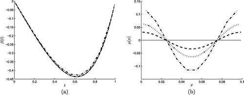
Figure 1. The analytical (—–) and numerical results for (a) $\mathit{\beta }(t)$ and (b) $\mathit{\mu }(x)$ obtained using the BEM for the direct problem with $N=N_0\in \{10(-·-),20(\cdots ),40(---)\}$, for Example 1.

Next we consider the inverse problem given by Equations (2.1(2.1) $$\begin{array}{c}\hfill {\displaystyle \frac{\mathit{\partial }u}{\mathit{\partial }t}}(x,t)={\displaystyle \frac{{\mathit{\partial }}^{2}u}{\mathit{\partial }{x}^2}}(x,t)+r(t)s(x),(x,t)\in D_T,\end{array}$$(2.1) ), (2.3(2.3) $$\begin{array}{c}\hfill {\displaystyle \frac{\mathit{\partial }u}{\mathit{\partial }x}}(0,t)={\displaystyle \frac{\mathit{\partial }u}{\mathit{\partial }x}}(L,t)=0,t\in [0,T],\end{array}$$(2.3) ), (2.6(2.6) $$\begin{array}{c}\hfill s(X_0)=\mathit{\alpha }.\end{array}$$(2.6) ) with $\mathit{\alpha }=s(1/20)=-40$ specified, (5.3(5.3) $$\begin{array}{c}\hfill \mathit{\phi }(x)=u(x,0)=0,x\in [0,L].\end{array}$$(5.3) ) and (5.6(5.6) $$\begin{array}{c}\hfill \mathit{\beta }(t)=u(1/20,t)=-(t-t^2)e^t,\mathit{\mu }(x)=u(x,1)=0,\mathit{\alpha }=s(1/20)=-40.\end{array}$$(5.6) ). The numerical solution is obtained, as described in Section 4, by minimizing the objective function (4.1(4.1) $$\begin{array}{c}\hfill {\mathbb{F}}_0(r,s):=\sum _{i=1}^N{\left(u(X_0,{\tilde{t}}_i)-\mathit{\beta }({\tilde{t}}_i)\right)}^2+\sum _{k=1}^{N_0}{\left(u({\tilde{x}}_k,T)-\mathit{\mu }({\tilde{x}}_k)\right)}^2+{(s(X_0)-\mathit{\alpha })}^2.\end{array}$$(4.1) ). Preliminary numerical investigations showed that the initial guesses ${\underline{r}}_0$ and ${\underline{s}}_0$ cannot be so arbitrary in order for the minimization process to converge. After many trials, we decided to illustrate the numerical results obtained by considering the initial guess as(5.7) $$\begin{array}{c}\hfill {\underline{r}}_0=\underline{r}+{\underline{\mathit{ϵ}}}_r,{\underline{s}}_0=\underline{s}+{\underline{\mathit{ϵ}}}_s,\end{array}$$(5.7)

where $\underline{r}$ and $\underline{s}$ are given by (5.4(5.4) $$\begin{array}{c}\hfill r(t)=-{\displaystyle \frac{e^t}{40}}\left(400{\mathit{\pi }}^2{t}^2-400{\mathit{\pi }}^{2}t+t^2+t-1\right),s(x)=40cos(20\mathit{\pi }x).\end{array}$$(5.4) ), and ${\underline{\mathit{ϵ}}}_r=\mathrm{random}(\mathrm{Normal},0,{\mathit{\sigma }}_r,N,1)$ and ${\underline{\mathit{ϵ}}}_s=\mathrm{random}(\mathrm{Normal},0,{\mathit{\sigma }}_s,N_0,1)$ are random variables generated by the MATLAB command for normal distributions with mean zero and the standard deviations ${\mathit{\sigma }}_r$ and ${\mathit{\sigma }}_s$, respectively, given by(5.8) $$\begin{array}{c}\hfill {\displaystyle {\mathit{\sigma }}_r=p_0\times \underset{t\in [0,T]}{max}|r(t)|,{\mathit{\sigma }}_s=p_0\times \underset{x\in [0,L]}{max}|s(x)|,}\end{array}$$(5.8)

where $p_0$ is a percentage of perturbation. The intention here was that the initial guesses (5.7(5.7) $$\begin{array}{c}\hfill {\underline{r}}_0=\underline{r}+{\underline{\mathit{ϵ}}}_r,{\underline{s}}_0=\underline{s}+{\underline{\mathit{ϵ}}}_s,\end{array}$$(5.7) ) are understood as some general priors for the unknowns presumed to have been obtained experimentally from some simple but rather inaccurate practical measurement. Hereafter, unless otherwise specified, we present results obtained with $p_0=100\%$ perturbed initial guess (which is quite far from the exact solution (5.4(5.4) $$\begin{array}{c}\hfill r(t)=-{\displaystyle \frac{e^t}{40}}\left(400{\mathit{\pi }}^2{t}^2-400{\mathit{\pi }}^{2}t+t^2+t-1\right),s(x)=40cos(20\mathit{\pi }x).\end{array}$$(5.4) )) and $N=N_0=20$, and use the MATLAB optimization toolbox lsqnonlin with TolFun = TolX = ${10}^{-6}$ to solve the inverse problem.

Figure 2. (a) The objective function ${\mathbb{F}}_0$ and the numerical results for (b) r(t), (c) s(x), (d) u(0, t), (e) u(0.1, t) obtained with no regularization $(-·-)$, for exact data for Example 1. The corresponding analytical solutions are shown by continuous line (—–) in (b)–(e) and the $p_0=100\%$ perturbed initial guesses are shown by dotted line $(\cdots )$ in (b) and (c).

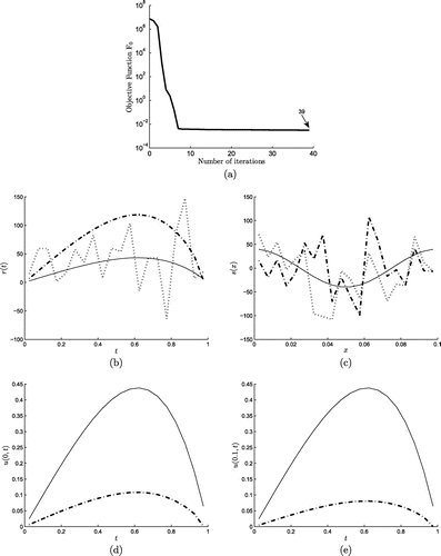
Figure 3. The numerical results for (a) r(t), (b) s(x), (c) u(0, t), (d) u(0.1, t) obtained with the first-order regularization $(\cdots )$ and the second-order regularization $(---)$ with regularization parameter $\mathit{\lambda }={10}^{-5}$, for exact data for Example 1. The corresponding analytical solutions are shown by continuous line (—–).

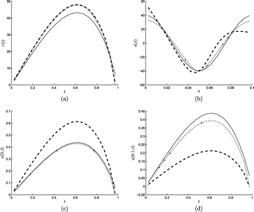
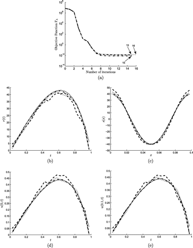
Figure 2(a) shows the unregularized objective function ${\mathbb{F}}_0$ which converges in 39 iterations and the numerical results for $r(t),s(x),u(0,t),u(0.1,t)$ are displayed in Figures 2(b)–(e), respectively. As we can see in these figures, the numerical results are inaccurate and partially unstable in Figure 2(c).

In order to improve the accuracy and stability, we apply a Tikhonov regularization process based on minimizing the penalised objective function(5.9) $$\begin{array}{c}\hfill {\mathbb{F}}_{\mathit{\lambda }}(\underline{r},\underline{s}):={\mathbb{F}}_0(\underline{r},\underline{s})+\mathit{\lambda }\left(\Vert R\underline{r}{\Vert }^2+{\Vert R\underline{s}\Vert }^2\right),\end{array}$$(5.9)

where $\mathit{\lambda }>0$ is a regularization parameter to be prescribed, and R is a (differential) regularizing matrix. Initially, we have applied the first- and second-order regularizations based on minimizing the objective function (5.9(5.9) $$\begin{array}{c}\hfill {\mathbb{F}}_{\mathit{\lambda }}(\underline{r},\underline{s}):={\mathbb{F}}_0(\underline{r},\underline{s})+\mathit{\lambda }\left(\Vert R\underline{r}{\Vert }^2+{\Vert R\underline{s}\Vert }^2\right),\end{array}$$(5.9) ) as(5.10) $$\begin{array}{cc}& {\mathbb{F}}_{\mathit{\lambda }}(\underline{r},\underline{s})={\mathbb{F}}_0(\underline{r},\underline{s})+\mathit{\lambda }\left(\sum _{i=1}^{N-1}{(r_{i+1}-r_i)}^2+\sum _{k=1}^{N_0-1}{(s_{k+1}-s_k)}^2\right),\hfill \end{array}$$(5.10) (5.11) $$\begin{array}{cc}& {\mathbb{F}}_{\mathit{\lambda }}(\underline{r},\underline{s})={\mathbb{F}}_0(\underline{r},\underline{s})+\mathit{\lambda }\left(\sum _{i=2}^{N-1}{(-r_{i+1}+2r_i-r_{i-1})}^2+\sum _{k=2}^{N_0-1}{(-s_{k+1}+2s_k-s_{k-1})}^2\right),\hfill \end{array}$$(5.11)

respectively. By trial and error, among various regularization parameters $\mathit{\lambda }\in \{{10}^{-9},\dots ,{10}^2\}$, we have found, as best illustrative results, those obtained with $\mathit{\lambda }={10}^{-5}$ which are shown in Figure 3. As we can see in this figure, applying orders one or two regularizations (5.10(5.10) $$\begin{array}{cc}& {\mathbb{F}}_{\mathit{\lambda }}(\underline{r},\underline{s})={\mathbb{F}}_0(\underline{r},\underline{s})+\mathit{\lambda }\left(\sum _{i=1}^{N-1}{(r_{i+1}-r_i)}^2+\sum _{k=1}^{N_0-1}{(s_{k+1}-s_k)}^2\right),\hfill \end{array}$$(5.10) ) or (5.11(5.11) $$\begin{array}{cc}& {\mathbb{F}}_{\mathit{\lambda }}(\underline{r},\underline{s})={\mathbb{F}}_0(\underline{r},\underline{s})+\mathit{\lambda }\left(\sum _{i=2}^{N-1}{(-r_{i+1}+2r_i-r_{i-1})}^2+\sum _{k=2}^{N_0-1}{(-s_{k+1}+2s_k-s_{k-1})}^2\right),\hfill \end{array}$$(5.11) ) yield stable, but rather inaccurate results, especially near the endpoints of the intervals of definition of the functions involved. In order to improve on these inaccuracies we have then investigated a hybrid combination of first- and second- order regularizations given by(5.12) $$\begin{array}{cc}\hfill {\mathbb{F}}_{\mathit{\lambda }}(\underline{r},\underline{s})& ={\mathbb{F}}_0(\underline{r},\underline{s})+\mathit{\lambda }({(r_1-r_2)}^2+{(-r_{N-1}+r_N)}^2+\sum _{i=2}^{N-1}{(-r_{i+1}+2r_i-r_{i-1})}^2\hfill \\ \hfill & +{(s_1-s_2)}^2+{(-s_{N_0-1}+s_{N_0})}^2+\sum _{k=2}^{N_0-1}{(-s_{k+1}+2s_k-s_{k-1})}^2).\hfill \end{array}$$(5.12)

According to (5.9(5.9) $$\begin{array}{c}\hfill {\mathbb{F}}_{\mathit{\lambda }}(\underline{r},\underline{s}):={\mathbb{F}}_0(\underline{r},\underline{s})+\mathit{\lambda }\left(\Vert R\underline{r}{\Vert }^2+{\Vert R\underline{s}\Vert }^2\right),\end{array}$$(5.9) ) and (5.12(5.12) $$\begin{array}{cc}\hfill {\mathbb{F}}_{\mathit{\lambda }}(\underline{r},\underline{s})& ={\mathbb{F}}_0(\underline{r},\underline{s})+\mathit{\lambda }({(r_1-r_2)}^2+{(-r_{N-1}+r_N)}^2+\sum _{i=2}^{N-1}{(-r_{i+1}+2r_i-r_{i-1})}^2\hfill \\ \hfill & +{(s_1-s_2)}^2+{(-s_{N_0-1}+s_{N_0})}^2+\sum _{k=2}^{N_0-1}{(-s_{k+1}+2s_k-s_{k-1})}^2).\hfill \end{array}$$(5.12) ), the differential regularization matrix R is given by(5.13) $$\begin{array}{cc}\hfill R& =\left[\begin{array}{cccccc}1& -1& 0& 0& .& 0\\ -1& 2& -1& 0& .& 0\\ 0& -1& 2& -1& .& 0\\ .& .& .& .& .& 0\\ 0& 0& 0& -1& 2& -1\\ 0& 0& 0& 0& -1& 1\\ \end{array}\right].\hfill \end{array}$$(5.13)

In the regularization process, we need to choose an appropriate regularization parameter $\mathit{\lambda }$ which balances accuracy and stability. Here, we use the L-curve method to find the regularization parameter $\mathit{\lambda }$. Figure 4(a) shows the L-curve obtained by plotting the solution norm $\sqrt{\Vert R\underline{r}{\Vert }^2+{\Vert R\underline{s}\Vert }^2}$ vs. the residual norm $\sqrt{{\mathbb{F}}_0(\underline{r},\underline{s})}$ for various values of $\mathit{\lambda }$ when R is given by (5.13(5.13) $$\begin{array}{cc}\hfill R& =\left[\begin{array}{cccccc}1& -1& 0& 0& .& 0\\ -1& 2& -1& 0& .& 0\\ 0& -1& 2& -1& .& 0\\ .& .& .& .& .& 0\\ 0& 0& 0& -1& 2& -1\\ 0& 0& 0& 0& -1& 1\\ \end{array}\right].\hfill \end{array}$$(5.13) ). From this figure it can be seen that the corner of the L-curve occurs nearby $\mathit{\lambda }={10}^{-5}$, with other appropriate values between the wide range ${10}^{-6}$ to ${10}^{-4}$. With this value of the regularization parameter the numerical results are shown in Figures 4(b)–(f). From Figure 4(b) it can be seen that convergence for the regularized objective function ${\mathbb{F}}_{\mathit{\lambda }}$ is achieved within 15 iterations. Also, in comparison with the previous Figures 3(c)–(f), very good agreement between the exact and the regularized numerical solutions is now obtained, as illustrated in Figures 4(c)–(f). All results are summarized in terms of the RMSE (5.1(5.1) $$\begin{array}{cc}\hfill {\text{RMSE}}_t& =\sqrt{{\displaystyle {\displaystyle \frac{1}{N}}\sum _{i=1}^N{\left(\mathrm{Exact}({\tilde{t}}_i)-\mathrm{Numerical}({\tilde{t}}_i)\right)}^2}},\hfill \end{array}$$(5.1) ) and (5.2(5.2) $$\begin{array}{cc}\hfill {\text{RMSE}}_x& =\sqrt{{\displaystyle {\displaystyle \frac{1}{N_0}}\sum _{k=1}^{N_0}{\left(\mathrm{Exact}({\tilde{x}}_k)-\mathrm{Numerical}({\tilde{x}}_k)\right)}^2}}.\hfill \end{array}$$(5.2) ) in Table 2. Various initial guesses (5.7(5.7) $$\begin{array}{c}\hfill {\underline{r}}_0=\underline{r}+{\underline{\mathit{ϵ}}}_r,{\underline{s}}_0=\underline{s}+{\underline{\mathit{ϵ}}}_s,\end{array}$$(5.7) ) with $p_0\in \{40,60,80,100\}\%$ in (5.8(5.8) $$\begin{array}{c}\hfill {\displaystyle {\mathit{\sigma }}_r=p_0\times \underset{t\in [0,T]}{max}|r(t)|,{\mathit{\sigma }}_s=p_0\times \underset{x\in [0,L]}{max}|s(x)|,}\end{array}$$(5.8) ) have been investigated in order to test the robustness of the minimization procedure with respect to the independence on the initial guess. From Table 2 it can be seen that whilst the choice of the initial guess seems to matter for the accuracy of the unregularized solution, this restriction disappears when regularization with $\mathit{\lambda }={10}^{-5}$ is imposed. This shows that the numerical regularization method employed is robust with respect to the independence on the initial guess.

Table 2. The RMSE (5.1(5.1) $$\begin{array}{cc}\hfill {\text{RMSE}}_t& =\sqrt{{\displaystyle {\displaystyle \frac{1}{N}}\sum _{i=1}^N{\left(\mathrm{Exact}({\tilde{t}}_i)-\mathrm{Numerical}({\tilde{t}}_i)\right)}^2}},\hfill \end{array}$$(5.1) ) and (5.2(5.2) $$\begin{array}{cc}\hfill {\text{RMSE}}_x& =\sqrt{{\displaystyle {\displaystyle \frac{1}{N_0}}\sum _{k=1}^{N_0}{\left(\mathrm{Exact}({\tilde{x}}_k)-\mathrm{Numerical}({\tilde{x}}_k)\right)}^2}}.\hfill \end{array}$$(5.2) ) for $r(t),s(x),u(0,t),u(0.1,t)$ for exact data for Example 1.

$p_0$	$\mathit{\lambda }$	r(t)	s(x)	u(0, t)	u(0.1, t)
40%	0	6.349	18.47	4.72E$-$2	3.27E$-$2
	${10}^{-5}$	1.528	0.819	1.49E$-$2	1.53E$-$2
60%	0	9.752	26.70	1.14E$-$1	8.12E$-$2
	${10}^{-5}$	1.513	0.767	1.48E$-$2	1.50E$-$2
80%	0	25.83	44.93	1.99E$-$1	2.74E$-$1
	${10}^{-5}$	1.526	0.812	1.48E$-$2	1.47E$-$2
100%	0	53.70	54.24	2.34E$-$1	2.54E$-$1
	${10}^{-5}$	1.529	0.819	1.47E$-$2	1.48E$-$2

Figure 4. (a) The L-curve criterion, (b) the objective function ${\mathbb{F}}_{\mathit{\lambda }}$, and the numerical results $(-\circ -)$for (c) r(t), (d) s(x), (e) u(0, t), (f) u(0.1, t) obtained with the hybrid-order regularization (5.12(5.12) $$\begin{array}{cc}\hfill {\mathbb{F}}_{\mathit{\lambda }}(\underline{r},\underline{s})& ={\mathbb{F}}_0(\underline{r},\underline{s})+\mathit{\lambda }({(r_1-r_2)}^2+{(-r_{N-1}+r_N)}^2+\sum _{i=2}^{N-1}{(-r_{i+1}+2r_i-r_{i-1})}^2\hfill \\ \hfill & +{(s_1-s_2)}^2+{(-s_{N_0-1}+s_{N_0})}^2+\sum _{k=2}^{N_0-1}{(-s_{k+1}+2s_k-s_{k-1})}^2).\hfill \end{array}$$(5.12) ) with regularization parameter $\mathit{\lambda }={10}^{-5}$ suggested by L-curve, for exact data for Example 1. The corresponding analytical solutions are shown by continuous line (—–) in (c)–(f).

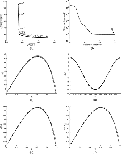
Figure 5. (a) The objective function ${\mathbb{F}}_{\mathit{\lambda }}$ and the numerical results for (b) r(t), (c) s(x), (d) u(0, t), (e) u(0.1, t) obtained with the hybrid-order regularization (5.12(5.12) $$\begin{array}{cc}\hfill {\mathbb{F}}_{\mathit{\lambda }}(\underline{r},\underline{s})& ={\mathbb{F}}_0(\underline{r},\underline{s})+\mathit{\lambda }({(r_1-r_2)}^2+{(-r_{N-1}+r_N)}^2+\sum _{i=2}^{N-1}{(-r_{i+1}+2r_i-r_{i-1})}^2\hfill \\ \hfill & +{(s_1-s_2)}^2+{(-s_{N_0-1}+s_{N_0})}^2+\sum _{k=2}^{N_0-1}{(-s_{k+1}+2s_k-s_{k-1})}^2).\hfill \end{array}$$(5.12) ) with regularization parameter $\mathit{\lambda }={10}^{-5}$ for $P\in \{1(-·-),3(\cdots ),5(---)\}\%$ noisy data for Example 1. The corresponding analytical solutions are shown by continuous line (—–) in (b)–(e).

To test the stability of the BEM combined with the nonlinear regularization, we solve the inverse problem when random noises defined as(5.14) $$\begin{array}{c}\hfill {\underline{\mathit{ϵ}}}_{\mathit{\beta }}^P=\mathrm{random}(\mathrm{Normal},0,{\mathit{\sigma }}_{\mathit{\beta }}^P,N,1),{\underline{\mathit{ϵ}}}_{\mathit{\mu }}^P=\mathrm{random}(\mathrm{Normal},0,{\mathit{\sigma }}_{\mathit{\mu }}^P,N_0,1),\end{array}$$(5.14)

are added to the input functions $\mathit{\beta }(t)$ and $\mathit{\mu }(x)$, respectively, where P represents the percentage of noise with which the measured data (2.4(2.4) $$\begin{array}{c}\hfill u(X_0,t)=\mathit{\beta }(t),t\in [0,T],\end{array}$$(2.4) ) and (2.5(2.5) $$\begin{array}{c}\hfill u(x,T)=\mathit{\mu }(x),x\in [0,L],\end{array}$$(2.5) ) is contaminated. In (5.14(5.14) $$\begin{array}{c}\hfill {\underline{\mathit{ϵ}}}_{\mathit{\beta }}^P=\mathrm{random}(\mathrm{Normal},0,{\mathit{\sigma }}_{\mathit{\beta }}^P,N,1),{\underline{\mathit{ϵ}}}_{\mathit{\mu }}^P=\mathrm{random}(\mathrm{Normal},0,{\mathit{\sigma }}_{\mathit{\mu }}^P,N_0,1),\end{array}$$(5.14) ), the standard deviations ${\mathit{\sigma }}_{\mathit{\beta }}^P$ and ${\mathit{\sigma }}_{\mathit{\mu }}^P$ are given by(5.15) $$\begin{array}{c}\hfill {\mathit{\sigma }}_{\mathit{\beta }}^P=P\times \underset{t\in [0,T]}{max}|\mathit{\beta }(t)|,{\mathit{\sigma }}_{\mathit{\mu }}^P=P\times \underset{x\in [0,L]}{max}|\mathit{\mu }(x)|.\end{array}$$(5.15)

Then $\underline{\mathit{\beta }}$ and $\underline{\mathit{\mu }}$ in (4.3(4.3) $$\begin{array}{cc}\hfill {\mathbb{F}}_0(\underline{r},\underline{s})& =\Vert -B^I{B}^{-1}(C\underline{\mathit{\phi }}+D^r\underline{s})+C^I\underline{\mathit{\phi }}+{D^r}^I\underline{s}-\underline{\mathit{\beta }}{\Vert }^2\hfill \\ \hfill & +\Vert -B^{II}{B}^{-1}(C\underline{\mathit{\phi }}+D^r\underline{s})+C^{II}\underline{\mathit{\phi }}+{D^r}^{II}\underline{s}-\underline{\mathit{\mu }}{\Vert }^2+{(s(X_0)-\mathit{\alpha })}^2,\hfill \end{array}$$(4.3) ) are replaced by their noisy perturbations(5.16) $$\begin{array}{c}\hfill {\underline{\mathit{\beta }}}^P=\underline{\mathit{\beta }}+{\underline{\mathit{ϵ}}}_{\mathit{\beta }}^P,{\underline{\mathit{\mu }}}^P=\underline{\mathit{\mu }}+{\underline{\mathit{ϵ}}}_{\mathit{\mu }}^P.\end{array}$$(5.16)

The numerical results obtained with $\mathit{\lambda }={10}^{-5}$, (suggested by the L-curve criterion) are illustrated in Figure 5. From Figure 5(a) it can be seen that convergence of the objective functional (5.12(5.12) $$\begin{array}{cc}\hfill {\mathbb{F}}_{\mathit{\lambda }}(\underline{r},\underline{s})& ={\mathbb{F}}_0(\underline{r},\underline{s})+\mathit{\lambda }({(r_1-r_2)}^2+{(-r_{N-1}+r_N)}^2+\sum _{i=2}^{N-1}{(-r_{i+1}+2r_i-r_{i-1})}^2\hfill \\ \hfill & +{(s_1-s_2)}^2+{(-s_{N_0-1}+s_{N_0})}^2+\sum _{k=2}^{N_0-1}{(-s_{k+1}+2s_k-s_{k-1})}^2).\hfill \end{array}$$(5.12) ) is rapidly achieved within 15–16 iterations for $P\in \{1,3,5\}\%$. Furthermore, Figures 5(b)–(e) show that stable and accurate numerical results are obtained for all amounts of noise P. Also, as expected, the numerical solutions become more accurate as the amount of noise P decreases.

5.2. Example 2

In Example 1, all conditions for the existence and uniqueness of Theorem 1 were satisfied. We now consider an example which has the analytical solution,[11](5.17) $$\begin{array}{c}\hfill u(x,t)=(e^{3t}-e^{-t})cos(x),(x,t)\in {\overline{D}}_T=[0,\mathit{\pi }]\times [0,0.3],\end{array}$$(5.17) (5.18) $$\begin{array}{c}\hfill r(t)=e^{3t},s(x)=4cos(x),t\in (0,0.3),x\in (0,\mathit{\pi }),\end{array}$$(5.18)

where $T=0.3,L=\mathit{\pi }$. One can easily check that the homogeneous Neumann conditions (2.3(2.3) $$\begin{array}{c}\hfill {\displaystyle \frac{\mathit{\partial }u}{\mathit{\partial }x}}(0,t)={\displaystyle \frac{\mathit{\partial }u}{\mathit{\partial }x}}(L,t)=0,t\in [0,T],\end{array}$$(2.3) ) are satisfied and that the initial condition (2.2(2.2) $$\begin{array}{c}\hfill u(x,0)=\mathit{\phi }(x),x\in [0,L],\end{array}$$(2.2) ) is homogeneous and given by (5.3(5.3) $$\begin{array}{c}\hfill \mathit{\phi }(x)=u(x,0)=0,x\in [0,L].\end{array}$$(5.3) ). Taking also $X_0=0.75$ we obtain that the input data (2.4(2.4) $$\begin{array}{c}\hfill u(X_0,t)=\mathit{\beta }(t),t\in [0,T],\end{array}$$(2.4) )–(2.6(2.6) $$\begin{array}{c}\hfill s(X_0)=\mathit{\alpha }.\end{array}$$(2.6) ) are given by(5.19) $$\begin{array}{c}\hfill \left\{\begin{array}{cc}& \mathit{\beta }(t)=u(0.75,t)=(e^{3t}-e^{-t})cos(0.75),\hfill \\ \hfill & \mathit{\mu }(x)=u(x,0.3)=(e^{0.9}-e^{-0.3})cos(x),\hfill \\ \hfill & \mathit{\alpha }=s(0.75)=4cos(0.75).\hfill \end{array}\right.\end{array}$$(5.19)

From (5.3(5.3) $$\begin{array}{c}\hfill \mathit{\phi }(x)=u(x,0)=0,x\in [0,L].\end{array}$$(5.3) ) and (5.19(5.19) $$\begin{array}{c}\hfill \left\{\begin{array}{cc}& \mathit{\beta }(t)=u(0.75,t)=(e^{3t}-e^{-t})cos(0.75),\hfill \\ \hfill & \mathit{\mu }(x)=u(x,0.3)=(e^{0.9}-e^{-0.3})cos(x),\hfill \\ \hfill & \mathit{\alpha }=s(0.75)=4cos(0.75).\hfill \end{array}\right.\end{array}$$(5.19) ) we have $\mathit{\alpha }=d=4cos(0.75)\ne 0,\mathit{\phi }(x)\equiv 0,m=e^{0.9}\ne 0,\mathit{\theta }(x)=(e^{0.9}-e^{-0.3})sin(x),{\mathit{\lambda }}_1=5.3719,{\mathit{\lambda }}_2=0.2518,{\mathit{\lambda }}_3=24.928,z_0=-8.6813,{\mathit{\lambda }}_4=14.654$. One can then observe that the conditions (i) and (ii) of Theorem 1 are satisfied, but the condition (iii) has been violated. Whilst a solution obviously exists, as given by Equations (5.17(5.17) $$\begin{array}{c}\hfill u(x,t)=(e^{3t}-e^{-t})cos(x),(x,t)\in {\overline{D}}_T=[0,\mathit{\pi }]\times [0,0.3],\end{array}$$(5.17) ) and (5.18(5.18) $$\begin{array}{c}\hfill r(t)=e^{3t},s(x)=4cos(x),t\in (0,0.3),x\in (0,\mathit{\pi }),\end{array}$$(5.18) ), one cannot guarantee yet that this solution is unique.

Figure 6. The analytical (—–) and numerical results for (a) $\mathit{\beta }(t)$ and (b) $\mathit{\mu }(x)$ obtained using the BEM for the direct problem with $N=N_0\in \{5(-·-),10(\cdots ),20(---)\}$, for Example 2.

We have solved first the direct problem given by Equations (2.1(2.1) $$\begin{array}{c}\hfill {\displaystyle \frac{\mathit{\partial }u}{\mathit{\partial }t}}(x,t)={\displaystyle \frac{{\mathit{\partial }}^{2}u}{\mathit{\partial }{x}^2}}(x,t)+r(t)s(x),(x,t)\in D_T,\end{array}$$(2.1) ) (with r and s given by (5.18(5.18) $$\begin{array}{c}\hfill r(t)=e^{3t},s(x)=4cos(x),t\in (0,0.3),x\in (0,\mathit{\pi }),\end{array}$$(5.18) )), (2.3(2.3) $$\begin{array}{c}\hfill {\displaystyle \frac{\mathit{\partial }u}{\mathit{\partial }x}}(0,t)={\displaystyle \frac{\mathit{\partial }u}{\mathit{\partial }x}}(L,t)=0,t\in [0,T],\end{array}$$(2.3) ) and (5.3(5.3) $$\begin{array}{c}\hfill \mathit{\phi }(x)=u(x,0)=0,x\in [0,L].\end{array}$$(5.3) ) using the BEM with various numbers of boundary elements $N=N_0\in \{5,10,20\}$ and the numerical results for $\mathit{\beta }(t)$ and $\mathit{\mu }(x)$ presented in Figure 6 show rapid convergence and excellent agreement with the analytical solution (5.19(5.19) $$\begin{array}{c}\hfill \left\{\begin{array}{cc}& \mathit{\beta }(t)=u(0.75,t)=(e^{3t}-e^{-t})cos(0.75),\hfill \\ \hfill & \mathit{\mu }(x)=u(x,0.3)=(e^{0.9}-e^{-0.3})cos(x),\hfill \\ \hfill & \mathit{\alpha }=s(0.75)=4cos(0.75).\hfill \end{array}\right.\end{array}$$(5.19) ). Afterwards, we have solved the inverse problem given by Equations (2.1(2.1) $$\begin{array}{c}\hfill {\displaystyle \frac{\mathit{\partial }u}{\mathit{\partial }t}}(x,t)={\displaystyle \frac{{\mathit{\partial }}^{2}u}{\mathit{\partial }{x}^2}}(x,t)+r(t)s(x),(x,t)\in D_T,\end{array}$$(2.1) ), (2.3(2.3) $$\begin{array}{c}\hfill {\displaystyle \frac{\mathit{\partial }u}{\mathit{\partial }x}}(0,t)={\displaystyle \frac{\mathit{\partial }u}{\mathit{\partial }x}}(L,t)=0,t\in [0,T],\end{array}$$(2.3) ), (5.3(5.3) $$\begin{array}{c}\hfill \mathit{\phi }(x)=u(x,0)=0,x\in [0,L].\end{array}$$(5.3) ) and (5.19(5.19) $$\begin{array}{c}\hfill \left\{\begin{array}{cc}& \mathit{\beta }(t)=u(0.75,t)=(e^{3t}-e^{-t})cos(0.75),\hfill \\ \hfill & \mathit{\mu }(x)=u(x,0.3)=(e^{0.9}-e^{-0.3})cos(x),\hfill \\ \hfill & \mathit{\alpha }=s(0.75)=4cos(0.75).\hfill \end{array}\right.\end{array}$$(5.19) ) in order to retrieve the temperature u(x, t) and the heat source components r(t) and s(x) given analytically by Equations (5.17(5.17) $$\begin{array}{c}\hfill u(x,t)=(e^{3t}-e^{-t})cos(x),(x,t)\in {\overline{D}}_T=[0,\mathit{\pi }]\times [0,0.3],\end{array}$$(5.17) ) and (5.18(5.18) $$\begin{array}{c}\hfill r(t)=e^{3t},s(x)=4cos(x),t\in (0,0.3),x\in (0,\mathit{\pi }),\end{array}$$(5.18) ), respectively. We have taken $N=N_0=20$ boundary elements and the arbitrary initial guesses ${\underline{r}}_0=\underline{0}$ and ${\underline{s}}_0=\underline{0}$.

We first consider the case of exact data. The convergence of the unregularized objective function ${\mathbb{F}}_0$ achieved within 56 iterations using the lsqnonlin routine with TolFun = TolX = ${10}^{-10}$ is illustrated in Figure 7(a). Also, the RMSEs (5.1(5.1) $$\begin{array}{cc}\hfill {\text{RMSE}}_t& =\sqrt{{\displaystyle {\displaystyle \frac{1}{N}}\sum _{i=1}^N{\left(\mathrm{Exact}({\tilde{t}}_i)-\mathrm{Numerical}({\tilde{t}}_i)\right)}^2}},\hfill \end{array}$$(5.1) ) and (5.2(5.2) $$\begin{array}{cc}\hfill {\text{RMSE}}_x& =\sqrt{{\displaystyle {\displaystyle \frac{1}{N_0}}\sum _{k=1}^{N_0}{\left(\mathrm{Exact}({\tilde{x}}_k)-\mathrm{Numerical}({\tilde{x}}_k)\right)}^2}}.\hfill \end{array}$$(5.2) ) of solutions r and s are shown in Figure 7(b). The numerical solutions for r and s obtained after 56 iterations are shown by dash-dot line $(-·-)$ in Figures 7(c) and (d), respectively. Very good agreement between the numerical and analytical solutions for s can be observed, whilst the numerical solution for r is stable but slightly away from the analytical solution. We then look more closely at Figure 7(b) and observe that the minimum of RMSEs is at iteration 31 instead of 56. Therefore, we have tried solving the inverse problem with the fixed iteration at 31, and the numerical results become more accurate, as illustrated by the circle markers $(\circ \circ \circ )$ in Figures 7(c) and (d). Further, we have applied the hybrid-order regularization procedure (5.12(5.12) $$\begin{array}{cc}\hfill {\mathbb{F}}_{\mathit{\lambda }}(\underline{r},\underline{s})& ={\mathbb{F}}_0(\underline{r},\underline{s})+\mathit{\lambda }({(r_1-r_2)}^2+{(-r_{N-1}+r_N)}^2+\sum _{i=2}^{N-1}{(-r_{i+1}+2r_i-r_{i-1})}^2\hfill \\ \hfill & +{(s_1-s_2)}^2+{(-s_{N_0-1}+s_{N_0})}^2+\sum _{k=2}^{N_0-1}{(-s_{k+1}+2s_k-s_{k-1})}^2).\hfill \end{array}$$(5.12) ) with the regularization parameter $\mathit{\lambda }=2\times {10}^{-4}$ (chosen by the trial and error) and the results are shown in Figures 8. Figure 8(a) displays the convergence of the regularized functional (5.12(5.12) $$\begin{array}{cc}\hfill {\mathbb{F}}_{\mathit{\lambda }}(\underline{r},\underline{s})& ={\mathbb{F}}_0(\underline{r},\underline{s})+\mathit{\lambda }({(r_1-r_2)}^2+{(-r_{N-1}+r_N)}^2+\sum _{i=2}^{N-1}{(-r_{i+1}+2r_i-r_{i-1})}^2\hfill \\ \hfill & +{(s_1-s_2)}^2+{(-s_{N_0-1}+s_{N_0})}^2+\sum _{k=2}^{N_0-1}{(-s_{k+1}+2s_k-s_{k-1})}^2).\hfill \end{array}$$(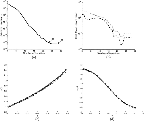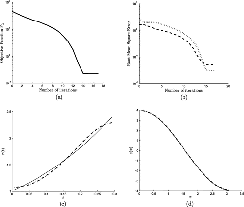5.12) ) achieved within 28 iterations. Also, results for RMSEs and the solutions for r and s are shown in Figures 8(b)–(d). From Figure 8(b) one can see that the minimum of the RMSEs occurs after 23 iterations. By comparing Figures 7 and 8 one can conclude that the inclusion of some small regularization yields slightly more accurate and stable results.

Table 3. The RMSEs (5.1(5.1) $$\begin{array}{cc}\hfill {\text{RMSE}}_t& =\sqrt{{\displaystyle {\displaystyle \frac{1}{N}}\sum _{i=1}^N{\left(\mathrm{Exact}({\tilde{t}}_i)-\mathrm{Numerical}({\tilde{t}}_i)\right)}^2}},\hfill \end{array}$$(5.1) ) and (5.2(5.2) $$\begin{array}{cc}\hfill {\text{RMSE}}_x& =\sqrt{{\displaystyle {\displaystyle \frac{1}{N_0}}\sum _{k=1}^{N_0}{\left(\mathrm{Exact}({\tilde{x}}_k)-\mathrm{Numerical}({\tilde{x}}_k)\right)}^2}}.\hfill \end{array}$$(5.2) ) for r(t) and s(x), for the noise levels $\mathit{\delta }\in \{0,0.01,0.1\}$, for Example 2.

Noise level	$\mathit{\lambda }$	No. of iterations	r(t)	s(x)
No noise	0	56	6.3068E–2	1.5492E–1
	0	31 (fixed)	2.6668E–2	1.4751E–1
	2E–4	28	5.6471E–2	1.1003E–1
	2E–4	23 (fixed)	1.9713E–2	6.4412E–2
$\mathit{\delta }=0.01$	4E–4	27	6.3004E–2	1.0886E–1
	4E–4	21 (fixed)	2.8829E–2	6.5281E–2
$\mathit{\delta }=0.1$	2	17	5.2212E–2	3.0714E–2

Figure 7. (a) The objective function ${\mathbb{F}}_0$, (b) the RMSEs (5.1(5.1) $$\begin{array}{cc}\hfill {\text{RMSE}}_t& =\sqrt{{\displaystyle {\displaystyle \frac{1}{N}}\sum _{i=1}^N{\left(\mathrm{Exact}({\tilde{t}}_i)-\mathrm{Numerical}({\tilde{t}}_i)\right)}^2}},\hfill \end{array}$$(5.1) ) and (5.2(5.2) $$\begin{array}{cc}\hfill {\text{RMSE}}_x& =\sqrt{{\displaystyle {\displaystyle \frac{1}{N_0}}\sum _{k=1}^{N_0}{\left(\mathrm{Exact}({\tilde{x}}_k)-\mathrm{Numerical}({\tilde{x}}_k)\right)}^2}}.\hfill \end{array}$$(5.2) ) for $r(t)(---)$ and $s(x)(\cdots )$ obtained with no regularization for exact data, and the numerical results for (c) r(t) and (d) s(x) obtained using the minimization process after 56 unfixed iterations $(-·-)$, and 31 fixed iterations $(\circ \circ \circ )$, for Example 2. The corresponding analytical solutions (5.18(5.18) $$\begin{array}{c}\hfill r(t)=e^{3t},s(x)=4cos(x),t\in (0,0.3),x\in (0,\mathit{\pi }),\end{array}$$(5.18) ) are shown by continuous line (—–) in (c) and (d).

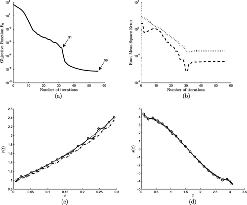
Figure 8. (a) The objective function ${\mathbb{F}}_{\mathit{\lambda }}$, (b) the RMSEs (5.1(5.1) $$\begin{array}{cc}\hfill {\text{RMSE}}_t& =\sqrt{{\displaystyle {\displaystyle \frac{1}{N}}\sum _{i=1}^N{\left(\mathrm{Exact}({\tilde{t}}_i)-\mathrm{Numerical}({\tilde{t}}_i)\right)}^2}},\hfill \end{array}$$(5.1) ) and (5.2(5.2) $$\begin{array}{cc}\hfill {\text{RMSE}}_x& =\sqrt{{\displaystyle {\displaystyle \frac{1}{N_0}}\sum _{k=1}^{N_0}{\left(\mathrm{Exact}({\tilde{x}}_k)-\mathrm{Numerical}({\tilde{x}}_k)\right)}^2}}.\hfill \end{array}$$(5.2) ) for $r(t)(---)$ and $s(x)(\cdots )$ obtained using the hybrid-order regularization (5.12(5.12) $$\begin{array}{cc}\hfill {\mathbb{F}}_{\mathit{\lambda }}(\underline{r},\underline{s})& ={\mathbb{F}}_0(\underline{r},\underline{s})+\mathit{\lambda }({(r_1-r_2)}^2+{(-r_{N-1}+r_N)}^2+\sum _{i=2}^{N-1}{(-r_{i+1}+2r_i-r_{i-1})}^2\hfill \\ \hfill & +{(s_1-s_2)}^2+{(-s_{N_0-1}+s_{N_0})}^2+\sum _{k=2}^{N_0-1}{(-s_{k+1}+2s_k-s_{k-1})}^2).\hfill \end{array}$$(5.12) ) with regularization parameter $\mathit{\lambda }=2\times {10}^{-4}$ for exact data, and the numerical results for (c) r(t) and (d) s(x) obtained using minimization process after 28 unfixed iterations $(-·-)$, and 23 fixed iterations $(\circ \circ \circ )$, for Example 2. The corresponding analytical solutions (5.18(5.18) $$\begin{array}{c}\hfill r(t)=e^{3t},s(x)=4cos(x),t\in (0,0.3),x\in (0,\mathit{\pi }),\end{array}$$(5.18) ) are shown by continuous line (—–) in (c) and (d).

Next, we consider the stability of the numerical solution when the noise is present in the input data (2.4(2.4) $$\begin{array}{c}\hfill u(X_0,t)=\mathit{\beta }(t),t\in [0,T],\end{array}$$(2.4) ) and (2.5(2.5) $$\begin{array}{c}\hfill u(x,T)=\mathit{\mu }(x),x\in [0,L],\end{array}$$(2.5) ). As in [11], the noise was defined by(5.20) $$\begin{array}{c}\hfill \left\{\begin{array}{cc}& {\mathit{\beta }}^{\mathit{\delta }}({\tilde{t}}_i)=\mathit{\beta }({\tilde{t}}_i)\left(1+{\displaystyle \frac{\mathit{\delta }}{\sqrt{{\sum }_{i=1}^N{\mathit{\beta }}^2({\tilde{t}}_i)}}}\mathrm{rand}(i)\right),i=\overline{1,N},\hfill \\ \hfill & {\mathit{\mu }}^{\mathit{\delta }}({\tilde{x}}_k)=\mathit{\mu }({\tilde{x}}_k)\left(1+{\displaystyle \frac{\mathit{\delta }}{\sqrt{{\sum }_{k=1}^N{\mathit{\mu }}^2({\tilde{x}}_k)}}}\mathrm{rand}(k)\right),k=\overline{1,N_0},\hfill \end{array}\right.\end{array}$$(5.20)

where $\mathrm{rand}(·)$ is a random variable generated by the MATLAB command from a normal distribution with mean zero and unit standard deviation, and $\mathit{\delta }$ represents the noise level. Remark that the noise (5.20(5.20) $$\begin{array}{c}\hfill \left\{\begin{array}{cc}& {\mathit{\beta }}^{\mathit{\delta }}({\tilde{t}}_i)=\mathit{\beta }({\tilde{t}}_i)\left(1+{\displaystyle \frac{\mathit{\delta }}{\sqrt{{\sum }_{i=1}^N{\mathit{\beta }}^2({\tilde{t}}_i)}}}\mathrm{rand}(i)\right),i=\overline{1,N},\hfill \\ \hfill & {\mathit{\mu }}^{\mathit{\delta }}({\tilde{x}}_k)=\mathit{\mu }({\tilde{x}}_k)\left(1+{\displaystyle \frac{\mathit{\delta }}{\sqrt{{\sum }_{k=1}^N{\mathit{\mu }}^2({\tilde{x}}_k)}}}\mathrm{rand}(k)\right),k=\overline{1,N_0},\hfill \end{array}\right.\end{array}$$(5.20) ) is multiplicative, whilst the noise in (5.16(5.16) $$\begin{array}{c}\hfill {\underline{\mathit{\beta }}}^P=\underline{\mathit{\beta }}+{\underline{\mathit{ϵ}}}_{\mathit{\beta }}^P,{\underline{\mathit{\mu }}}^P=\underline{\mathit{\mu }}+{\underline{\mathit{ϵ}}}_{\mathit{\mu }}^P.\end{array}$$(5.16) ) is additive. For $\mathit{\delta }=0.01$, Figure 9 illustrates the results obtained using the hybrid-order regularization (5.12(5.12) $$\begin{array}{cc}\hfill {\mathbb{F}}_{\mathit{\lambda }}(\underline{r},\underline{s})& ={\mathbb{F}}_0(\underline{r},\underline{s})+\mathit{\lambda }({(r_1-r_2)}^2+{(-r_{N-1}+r_N)}^2+\sum _{i=2}^{N-1}{(-r_{i+1}+2r_i-r_{i-1})}^2\hfill \\ \hfill & +{(s_1-s_2)}^2+{(-s_{N_0-1}+s_{N_0})}^2+\sum _{k=2}^{N_0-1}{(-s_{k+1}+2s_k-s_{k-1})}^2).\hfill \end{array}$$(5.12) ) with regularization parameter $\mathit{\lambda }=4\times {10}^{-4}$ (found by the trial and error). The convergence of the regularized objective function achieved within 27 iterations is shown in Figure 9(a), whilst the minimum RMSEs of r and s occur after 21 iterations, as can be seen in Figure 9(b). Numerical solutions for r and s obtained after 27 (unfixed) and 21 (fixed) iterations are displayed in Figures 9(c) and (d), respectively. As expected, the conclusions from Figure 9 obtained for a low level of noise $\mathit{\delta }=0.01$ are very much the same as the those from Figure 8 obtained for no noise $\mathit{\delta }=0$. From both Figures 8(c), (d) and 9(c), (d) one can observe that the numerical results are accurate and stable. Furthermore, there is little difference in the results obtained whether we stop (fix) the iteration process at the minimum of the RMSEs shown in Figures 8(b) and 9(b) or, if we let the iteration process running until converge of the regularized objective function is achieved.

Figure 9. (a) The objective function $F_{\mathit{\lambda }}$, (b) the RMSEs (5.1(5.1) $$\begin{array}{cc}\hfill {\text{RMSE}}_t& =\sqrt{{\displaystyle {\displaystyle \frac{1}{N}}\sum _{i=1}^N{\left(\mathrm{Exact}({\tilde{t}}_i)-\mathrm{Numerical}({\tilde{t}}_i)\right)}^2}},\hfill \end{array}$$(5.1) ) and (5.2(5.2) $$\begin{array}{cc}\hfill {\text{RMSE}}_x& =\sqrt{{\displaystyle {\displaystyle \frac{1}{N_0}}\sum _{k=1}^{N_0}{\left(\mathrm{Exact}({\tilde{x}}_k)-\mathrm{Numerical}({\tilde{x}}_k)\right)}^2}}.\hfill \end{array}$$(5.2) ) for $r(t)(---)$ and $s(x)(\cdots )$ obtained using the hybrid-order regularization (5.12(5.12) $$\begin{array}{cc}\hfill {\mathbb{F}}_{\mathit{\lambda }}(\underline{r},\underline{s})& ={\mathbb{F}}_0(\underline{r},\underline{s})+\mathit{\lambda }({(r_1-r_2)}^2+{(-r_{N-1}+r_N)}^2+\sum _{i=2}^{N-1}{(-r_{i+1}+2r_i-r_{i-1})}^2\hfill \\ \hfill & +{(s_1-s_2)}^2+{(-s_{N_0-1}+s_{N_0})}^2+\sum _{k=2}^{N_0-1}{(-s_{k+1}+2s_k-s_{k-1})}^2).\hfill \end{array}$$(5.12) ) with regularization parameter $\mathit{\lambda }=4\times {10}^{-4}$ for noise level $\mathit{\delta }=0.01$, and the numerical results for (c) r(t) and (d) s(x) obtained using the minimization process after 27 unfixed iterations $(-·-)$, and 21 fixed iterations $(\circ \circ \circ )$, for Example 2. The corresponding analytical solutions (5.18(5.18) $$\begin{array}{c}\hfill r(t)=e^{3t},s(x)=4cos(x),t\in (0,0.3),x\in (0,\mathit{\pi }),\end{array}$$(5.18) ) are shown by continuous line (—–) in (c) and (d).

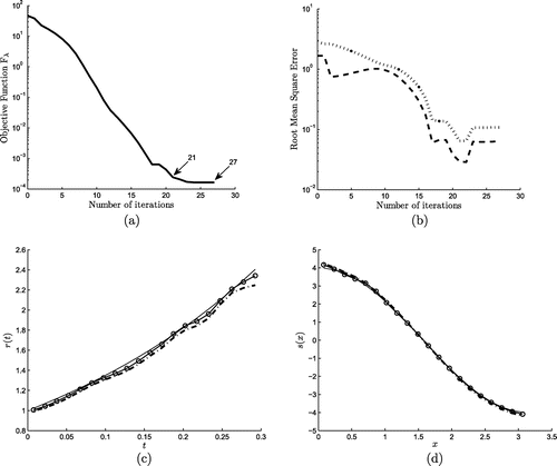
Figure 10. (a) The objective function $F_{\mathit{\lambda }}$, (b) the RMSEs (5.1(5.1) $$\begin{array}{cc}\hfill {\text{RMSE}}_t& =\sqrt{{\displaystyle {\displaystyle \frac{1}{N}}\sum _{i=1}^N{\left(\mathrm{Exact}({\tilde{t}}_i)-\mathrm{Numerical}({\tilde{t}}_i)\right)}^2}},\hfill \end{array}$$(5.1) ) and (5.2(5.2) $$\begin{array}{cc}\hfill {\text{RMSE}}_x& =\sqrt{{\displaystyle {\displaystyle \frac{1}{N_0}}\sum _{k=1}^{N_0}{\left(\mathrm{Exact}({\tilde{x}}_k)-\mathrm{Numerical}({\tilde{x}}_k)\right)}^2}}.\hfill \end{array}$$(5.2) ) for $r(t)(---)$ and $s(x)(\cdots )$ obtained using the hybrid-order regularization (5.12(5.12) $$\begin{array}{cc}\hfill {\mathbb{F}}_{\mathit{\lambda }}(\underline{r},\underline{s})& ={\mathbb{F}}_0(\underline{r},\underline{s})+\mathit{\lambda }({(r_1-r_2)}^2+{(-r_{N-1}+r_N)}^2+\sum _{i=2}^{N-1}{(-r_{i+1}+2r_i-r_{i-1})}^2\hfill \\ \hfill & +{(s_1-s_2)}^2+{(-s_{N_0-1}+s_{N_0})}^2+\sum _{k=2}^{N_0-1}{(-s_{k+1}+2s_k-s_{k-1})}^2).\hfill \end{array}$$(5.12) ) with regularization parameter $\mathit{\lambda }=2$ for noise level $\mathit{\delta }=0.1$, and the numerical results $(-·-)$ for (c) r(t) and (d) s(x) obtained using the minimization process after 17 (unfixed) iterations, for Example 2. The corresponding analytical solutions (5.18(5.18) $$\begin{array}{c}\hfill r(t)=e^{3t},s(x)=4cos(x),t\in (0,0.3),x\in (0,\mathit{\pi }),\end{array}$$(5.18) ) are shown by continuous line (—–) in (c) and (d).

Next, we consider a large amount of noise, such as $\mathit{\delta }=0.1$, included in (5.20(5.20) $$\begin{array}{c}\hfill \left\{\begin{array}{cc}& {\mathit{\beta }}^{\mathit{\delta }}({\tilde{t}}_i)=\mathit{\beta }({\tilde{t}}_i)\left(1+{\displaystyle \frac{\mathit{\delta }}{\sqrt{{\sum }_{i=1}^N{\mathit{\beta }}^2({\tilde{t}}_i)}}}\mathrm{rand}(i)\right),i=\overline{1,N},\hfill \\ \hfill & {\mathit{\mu }}^{\mathit{\delta }}({\tilde{x}}_k)=\mathit{\mu }({\tilde{x}}_k)\left(1+{\displaystyle \frac{\mathit{\delta }}{\sqrt{{\sum }_{k=1}^N{\mathit{\mu }}^2({\tilde{x}}_k)}}}\mathrm{rand}(k)\right),k=\overline{1,N_0},\hfill \end{array}\right.\end{array}$$(5.20) ) and the numerical results are shown in Figure 10. First, one can observe from Figure 10(a) that the convergence of the objective function (5.12(5.12) $$\begin{array}{cc}\hfill {\mathbb{F}}_{\mathit{\lambda }}(\underline{r},\underline{s})& ={\mathbb{F}}_0(\underline{r},\underline{s})+\mathit{\lambda }({(r_1-r_2)}^2+{(-r_{N-1}+r_N)}^2+\sum _{i=2}^{N-1}{(-r_{i+1}+2r_i-r_{i-1})}^2\hfill \\ \hfill & +{(s_1-s_2)}^2+{(-s_{N_0-1}+s_{N_0})}^2+\sum _{k=2}^{N_0-1}{(-s_{k+1}+2s_k-s_{k-1})}^2).\hfill \end{array}$$(5.12) ) is rapidly achieved within 17 iterations and the monotonic decreasing curve has a somewhat different shape than that recorded in Figure 8(a) for no noise $\mathit{\delta }=0$ or in Figure 9(a) for a low amount noise $\mathit{\delta }=0.01$. Also, interestingly, unlike in Figures 8(b) and 9(b) where the RMSEs (5.1(5.1) $$\begin{array}{cc}\hfill {\text{RMSE}}_t& =\sqrt{{\displaystyle {\displaystyle \frac{1}{N}}\sum _{i=1}^N{\left(\mathrm{Exact}({\tilde{t}}_i)-\mathrm{Numerical}({\tilde{t}}_i)\right)}^2}},\hfill \end{array}$$(5.1) ) and (5.2(5.2) $$\begin{array}{cc}\hfill {\text{RMSE}}_x& =\sqrt{{\displaystyle {\displaystyle \frac{1}{N_0}}\sum _{k=1}^{N_0}{\left(\mathrm{Exact}({\tilde{x}}_k)-\mathrm{Numerical}({\tilde{x}}_k)\right)}^2}}.\hfill \end{array}$$(5.2) ) show a minimum before the iteration process has finished, in Figure 10(b) no such minimum occurs. Therefore, in Figures 10(c) and (d) we present only numerical results for r and s, respectively, obtained after 17 (unfixed) iterations.

From these figures it can be seen that the numerical solutions are stable, with an unexpected very high accuracy in predicting the s component in Figure 10(d). For completeness and clarity the RMSEs (5.1(5.1) $$\begin{array}{cc}\hfill {\text{RMSE}}_t& =\sqrt{{\displaystyle {\displaystyle \frac{1}{N}}\sum _{i=1}^N{\left(\mathrm{Exact}({\tilde{t}}_i)-\mathrm{Numerical}({\tilde{t}}_i)\right)}^2}},\hfill \end{array}$$(5.1) ) and (5.2(5.2) $$\begin{array}{cc}\hfill {\text{RMSE}}_x& =\sqrt{{\displaystyle {\displaystyle \frac{1}{N_0}}\sum _{k=1}^{N_0}{\left(\mathrm{Exact}({\tilde{x}}_k)-\mathrm{Numerical}({\tilde{x}}_k)\right)}^2}}.\hfill \end{array}$$(5.2) ) of Figures 7(b)–10(b) are given in numbers in Table 3. From this table and also, from Figure 10(b) it can be seen that for $\mathit{\delta }=0.1$ the component s(x) is predicted more accurately than the r(t) component, whilst for $\mathit{\delta }\in \{0,0.01\}$ in Figures 7(b), 8(b) and 9(b) this prediction is reversed.

Figure 11. The numerical results for (a) $\mathit{\beta }(t)$ and (b) $\mathit{\mu }(x)$ obtained using the BEM for the direct problem with $N=N_0\in \{10(-·-),20(\cdots ),40(---)\}$, for Example 3.

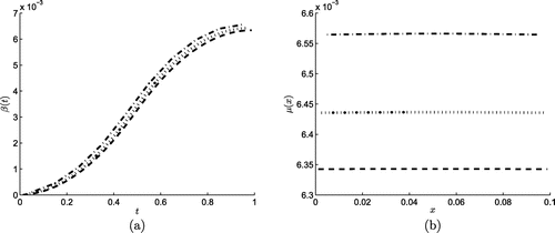
Figure 12. (a) The objective function $F_{\mathit{\lambda }}$ and the numerical results for (b) r(t) and (c) s(x) obtained with the hybrid-order regularization (5.12(5.12) $$\begin{array}{cc}\hfill {\mathbb{F}}_{\mathit{\lambda }}(\underline{r},\underline{s})& ={\mathbb{F}}_0(\underline{r},\underline{s})+\mathit{\lambda }({(r_1-r_2)}^2+{(-r_{N-1}+r_N)}^2+\sum _{i=2}^{N-1}{(-r_{i+1}+2r_i-r_{i-1})}^2\hfill \\ \hfill & +{(s_1-s_2)}^2+{(-s_{N_0-1}+s_{N_0})}^2+\sum _{k=2}^{N_0-1}{(-s_{k+1}+2s_k-s_{k-1})}^2).\hfill \end{array}$$(5.12) ) with regularization parameter $\mathit{\lambda }=2\times {10}^{-4}$ for $P=1\%(-·-),P=5\%(\cdots )$ and $P=10\%(---)$ noisy data for Example 3. The corresponding analytical solutions (5.21(5.21) $$\begin{array}{c}\hfill r(t)=\left\{\begin{array}{cc}t,\hfill & 0\le t\le 1/2\hfill \\ 1-t,\hfill & 1/2<t\le 1=T\hfill \end{array}\right.,s(x)=\left\{\begin{array}{cc}x,\hfill & 0\le x\le 1/20\hfill \\ 0.1-x,\hfill & 1/20<x\le 1/10=L\hfill \end{array}\right.,\end{array}$$(5.21) ) are shown by continuous line (—–) in (b) and (c).

Finally, we report that the numerical results presented in this subsection for Example 2 are comparable in terms of accuracy and stability with the numerical results obtained recently in [11] using a different method of successive approximants previously developed in [10].

5.3. Example 3

The previous examples possessed an analytical (smooth) solution available explicitly and they were tested in order to verify the accuracy and stability of the numerical method employed. In this subsection, we consider a severe test example represented by the non-smooth source components(5.21) $$\begin{array}{c}\hfill r(t)=\left\{\begin{array}{cc}t,\hfill & 0\le t\le 1/2\hfill \\ 1-t,\hfill & 1/2<t\le 1=T\hfill \end{array}\right.,s(x)=\left\{\begin{array}{cc}x,\hfill & 0\le x\le 1/20\hfill \\ 0.1-x,\hfill & 1/20<x\le 1/10=L\hfill \end{array}\right.,\end{array}$$(5.21)

where $L=1/10,T=1,X_0=1/20$. We also take the homogeneous initial temperature (5.3(5.3) $$\begin{array}{c}\hfill \mathit{\phi }(x)=u(x,0)=0,x\in [0,L].\end{array}$$(5.3) ). This example does not have an analytical solution for the temperature u(x, t) readily available. Therefore, in such a situation the data (2.4(2.4) $$\begin{array}{c}\hfill u(X_0,t)=\mathit{\beta }(t),t\in [0,T],\end{array}$$(2.4) ) and (2.5(2.5) $$\begin{array}{c}\hfill u(x,T)=\mathit{\mu }(x),x\in [0,L],\end{array}$$(2.5) ) is simulated numerically by solving the direct problem (2.1(2.1) $$\begin{array}{c}\hfill {\displaystyle \frac{\mathit{\partial }u}{\mathit{\partial }t}}(x,t)={\displaystyle \frac{{\mathit{\partial }}^{2}u}{\mathit{\partial }{x}^2}}(x,t)+r(t)s(x),(x,t)\in D_T,\end{array}$$(2.1) ) with the multiplicative source given by the product of the functions in (5.21(5.21) $$\begin{array}{c}\hfill r(t)=\left\{\begin{array}{cc}t,\hfill & 0\le t\le 1/2\hfill \\ 1-t,\hfill & 1/2<t\le 1=T\hfill \end{array}\right.,s(x)=\left\{\begin{array}{cc}x,\hfill & 0\le x\le 1/20\hfill \\ 0.1-x,\hfill & 1/20<x\le 1/10=L\hfill \end{array}\right.,\end{array}$$(5.21) ), subject to the homogeneous boundary and initial conditions (2.3(2.3) $$\begin{array}{c}\hfill {\displaystyle \frac{\mathit{\partial }u}{\mathit{\partial }x}}(0,t)={\displaystyle \frac{\mathit{\partial }u}{\mathit{\partial }x}}(L,t)=0,t\in [0,T],\end{array}$$(2.3) ) and (5.3(5.3) $$\begin{array}{c}\hfill \mathit{\phi }(x)=u(x,0)=0,x\in [0,L].\end{array}$$(5.3) ). The BEM numerical solutions for the data $\mathit{\beta }(t)=u(1/20,t)$ and $\mathit{\mu }(x)=u(x,1)$ are shown in Figure 11 for various numbers of boundary elements $N=N_0\in \{10,20,40\}$. From this figure the convergence of the numerical solution, as the number of boundary elements increases, can be observed.

Next we consider the inverse problem given by Equations (2.1(2.1) $$\begin{array}{c}\hfill {\displaystyle \frac{\mathit{\partial }u}{\mathit{\partial }t}}(x,t)={\displaystyle \frac{{\mathit{\partial }}^{2}u}{\mathit{\partial }{x}^2}}(x,t)+r(t)s(x),(x,t)\in D_T,\end{array}$$(2.1) ), (2.3(2.3) $$\begin{array}{c}\hfill {\displaystyle \frac{\mathit{\partial }u}{\mathit{\partial }x}}(0,t)={\displaystyle \frac{\mathit{\partial }u}{\mathit{\partial }x}}(L,t)=0,t\in [0,T],\end{array}$$(2.3) ), (2.6(2.6) $$\begin{array}{c}\hfill s(X_0)=\mathit{\alpha }.\end{array}$$(2.6) ) with $\mathit{\alpha }=s(1/20)=1/20$ specified, (5.3(5.3) $$\begin{array}{c}\hfill \mathit{\phi }(x)=u(x,0)=0,x\in [0,L].\end{array}$$(5.3) ), and the additional measured data (2.4(2.4) $$\begin{array}{c}\hfill u(X_0,t)=\mathit{\beta }(t),t\in [0,T],\end{array}$$(2.4) ) and (2.5(2.5) $$\begin{array}{c}\hfill u(x,T)=\mathit{\mu }(x),x\in [0,L],\end{array}$$(2.5) ) which has been simulated numerically in Figure 11. We pick from Figure 11 the numerical BEM solutions obtained with $N=N_0=20$ and we further perturb this data with noise, as in (5.16(5.16) $$\begin{array}{c}\hfill {\underline{\mathit{\beta }}}^P=\underline{\mathit{\beta }}+{\underline{\mathit{ϵ}}}_{\mathit{\beta }}^P,{\underline{\mathit{\mu }}}^P=\underline{\mathit{\mu }}+{\underline{\mathit{ϵ}}}_{\mathit{\mu }}^P.\end{array}$$(5.16) ). We took as initial guesses ${\underline{r}}_0={\underline{s}}_0=0$, and we initiated the iterative minimization process of the hybrid regularization functional (5.12(5.12) $$\begin{array}{cc}\hfill {\mathbb{F}}_{\mathit{\lambda }}(\underline{r},\underline{s})& ={\mathbb{F}}_0(\underline{r},\underline{s})+\mathit{\lambda }({(r_1-r_2)}^2+{(-r_{N-1}+r_N)}^2+\sum _{i=2}^{N-1}{(-r_{i+1}+2r_i-r_{i-1})}^2\hfill \\ \hfill & +{(s_1-s_2)}^2+{(-s_{N_0-1}+s_{N_0})}^2+\sum _{k=2}^{N_0-1}{(-s_{k+1}+2s_k-s_{k-1})}^2).\hfill \end{array}$$(5.12) ), as described in Example 1. 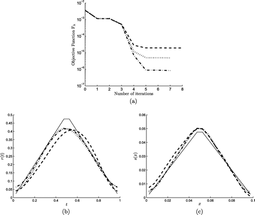The numerical results obtained with $\mathit{\lambda }=2\times {10}^{-4}$ (found by trial and error) are shown in Figure 12 for $P=\{1,5,10\}\%$ noise generated as in (5.16(5.16) $$\begin{array}{c}\hfill {\underline{\mathit{\beta }}}^P=\underline{\mathit{\beta }}+{\underline{\mathit{ϵ}}}_{\mathit{\beta }}^P,{\underline{\mathit{\mu }}}^P=\underline{\mathit{\mu }}+{\underline{\mathit{ϵ}}}_{\mathit{\mu }}^P.\end{array}$$(5.16) ). From Figure 12(a) it can be seen that the convergence of the functional (5.12(5.12) $$\begin{array}{cc}\hfill {\mathbb{F}}_{\mathit{\lambda }}(\underline{r},\underline{s})& ={\mathbb{F}}_0(\underline{r},\underline{s})+\mathit{\lambda }({(r_1-r_2)}^2+{(-r_{N-1}+r_N)}^2+\sum _{i=2}^{N-1}{(-r_{i+1}+2r_i-r_{i-1})}^2\hfill \\ \hfill & +{(s_1-s_2)}^2+{(-s_{N_0-1}+s_{N_0})}^2+\sum _{k=2}^{N_0-1}{(-s_{k+1}+2s_k-s_{k-1})}^2).\hfill \end{array}$$(5.12) ) is rapidly achieved within 7–8 iterations using the lsqnonlin routine with TolFun = TolX = ${10}^{-6}$. Also, Figures 12(b) and (c) show that stable and accurate numerical solutions for both r(t) and s(x) are obtained for all the amounts of noise P.

In closure, although not illustrated, we report that the same good performance has been recorded when attempting to reconstruct even discontinuous source components.

6. Conclusions

In this paper, inverse source problems with homogeneous Neumann boundary conditions together with specified interior and final time temperature measurements have been considered to find the space- and the time-dependent components of a multiplicative source function. The numerical discretization was based on the BEM combined with a Tikhonov regularization procedure. For a wide range of test example, the obtained results indicate that stable and accurate numerical solutions have been achieved. The identification of both multiplicative r(t)s(x) and additive $\mathit{\varphi }(t)+\mathit{\psi }(x)$ components of space- and time-dependent sources of the form $r(t)s(x)+\mathit{\varphi }(t)+\mathit{\psi }(x)$ can also be considered,[10] but its numerical implementation is deferred to a future work.

Acknowledgements

A. Hazanee would like to acknowledge the financial support received from the Ministry of Science and Technology of Thailand, and Prince of Songkla University Thailand, for pursuing her PhD at the University of Leeds.

Notes

No potential conflict of interest was reported by the authors.

References

- Erdem A, Lesnic D, Hasanov A. Identification of a spacewise dependent heat source. Appl. Math. Model. 2013;37:10231–10244.
- Farcas A, Lesnic D. The boundary element method for the determination of a heat source dependent on one variable. J. Eng. Math. 2006;54:375–388.
- Hasanov A. Identification of spacewise and time dependent source terms in 1D heat conduction equation from temperature measurement at final time. Int. J. Heat Mass Transfer. 2012;55:2069–2080.
- Hasanov A, Slodicka M. An analysis of inverse source problems with final measured out put data for the heat conduction equation: a semigroup approach. Appl. Math. Lett. 2013;26:207–214.
- Johansson BT, Lesnic D. A variational method for identifying a spacewise dependent heat source. IMA J. Appl. Math. 2007;72:748–760.
- Prilepko AI, Solov’ev VV. Solvability theorems and Rothe’s method for inverse problems for a parabolic equation. II. Differ. Equ. 1987;23:1341–1349.
- Solov’ev VV. Solvability of the inverse problem of finding a source, using overdetermination of the upper base for a parabolic equation. Differ. Equ. 1990;25:1114–1119.
- Bushuyev I. Global uniqueness for inverse parabolic problems with final observation. Inverse Prob. 1995;11:L11–L16.
- Hazanee A, Lesnic D. Reconstruction of an additive space- and time-dependent heat source. Eur. J. Comput. Mech. 2013;22:304–329.
- Savateev EG. On problems of determining the source function in a parabolic equation. J. Inverse Ill-Posed Prob. 1995;3:83–102.
- Shi C, Wang C, Wei T. Numerical solution for an inverse heat source problem by an iterative method. Appl. Math. Comput. 2014;244:577–597.
- Dym H, McKean H. Fourier series and integrals. New York (NY): Academic Press; 1985.
- Engl HW, Hanke M, Neubauer A. Regularization of inverse problems. Dordrecht: Kluwer Academic; 2000.