A Gaussian RBFs method with regularization for the numerical solution of inverse heat conduction problems

Abstract

In this paper, a recursion numerical technique is considered to solve the inverse heat conduction problems, with an unknown time-dependent heat source and the Neumann boundary conditions. The numerical solutions of the heat diffusion equations are constructed using the Gaussian radial basis functions. The details of algorithms in the one-dimensional and two-dimensional cases, involving the global or partial initial conditions, are proposed, respectively. The Tikhonov regularization method, with the generalized cross-validation criterion, is used to obtain more stable numerical results, since the linear systems are badly ill-conditioned. Moreover, we propose some results of the condition number estimates to a class of positive define matrices constructed by the Gaussian radial basis functions. Some numerical experiments are given to show that the presented schemes are favourably accurate and effective.

Keywords:

• Inverse heat conduction problem
• numerical recursion scheme
• time-dependent heat source
• radial basis functions
• Neumann boundary conditions
• regularization methods

AMS Subject Classifications:

• 65M32
• 65F22
• 65D05

1. Introduction

The inverse heat conduction problems (IHCPs) have been widely studied over last 40 years, which often arise in heat flux, industrial controlling models with heat propagation, etc. However, the inverse problems are unstable in nature, because the identified functions have to be determined from the observable data with measured errors, it means that IHCPs are ill-posed, any small errors for measurement values on some specified points can result in a large error to the solution of problems, and the resultant discretized matrix is ill-conditioned.[1,2]

In practice, many traditional numerical methods can either not handle such problems which possess high-dimensional data in many areas of science and engineering, or are limited to very special (regular) situations. But the meshfree methods are often better suited to deal with changes in the geometry of the domain of interest (e.g. free surfaces and large deformations) than classical discretization schemes, such as finite differences, finite elements or finite volumes. Another advantage of meshless techniques is independent from a mesh.[3] In general, the domain of the solution is often irregular, and the boundary conditions are of a mixed type,[4] in this case a solution of the problem is constructed using a set of radial basis functions (RBFs) to the corresponding partial differential equations (PDEs), this method leads to a meshless procedure in contrast to the traditional solution methods. However, the matrices which result from the discretization of the equations are usually ill-conditioned, especially in higher dimensional problems.[5] In this paper, we use the Tikhonov regularization method to overcome the ill-posedness of IHCPs.

Many numerical algorithms, for solving one-dimensional and multi-dimensional IHCPs, have been proposed during the last decades, including the finite difference method (FDM).[6–9] But FDM limits to solve the problems possessing very special regular domains and low-dimensional cases, and the property of mesh-dependent requires enormous computation cost for lots of grids or elements, so it can derive numerical instability. We can also refer to the method of fundamental solutions (MFS),[2,10–14] the most important advantage of MFS is an inherently meshless, and integration-free scheme for solving different PDEs,[12] but only the fundamental solution of the governing PDE is known, the MFS can be exploited in the given problems. It needs source points outside the domains, in which are not easy to be placed, and the constant number T is not chosen properly in the shift function.[15] In addition, the condition number of the resultant matrix is very large commonly, if the collocation points are picked more enough. In the literature, Dehghan et al. [16] developed a numerical method using radial basis functions to solve one-dimensional inverse heat conduction problem, with source control parameter and Dirichlet boundary conditions, Dehghan et al. [17,18], Saadatmandi et al. [19], Lakestani et al. [20] applied different numerical technologies to solve IHCPs involving unknown control parameter. Recently, Ma et al. [21] employed RBFs to solve a class of multi-dimensional inverse parabolic problems with control source parameter p(t). Xiong et al. [15] presented an alternative direct method, for solving inverse problems of determining space-wise and time-wise dependent heat source, in the heat diffusion equations. Dehghan et al. [22,23] proposed the meshless method of RBFs to solve a series of nonlinear high-dimensional PDEs, and obtained effective results. However, the investigated IHCPs, with the Neumann boundary conditions, are more difficult to be solved than ones involving only Dirichlet boundary conditions. We apply some properties of Gaussian RBFs, e.g. infinitely differentiable, to treat easily the Neumann boundary conditions in this paper.

The paper is organized as follows. In Section 2, the RBFs and regularization techniques are introduced. We consider a class of IHCPs with the time-dependent heat source term f(t) and the Neumann boundary conditions in one-dimensional and two-dimensional cases, and the numerical recursion schemes involving the global or partial initial condition cases are proposed in Sections 3 and 4, respectively. The condition number estimates of interpolation matrices, constructed by Gaussian RBFs, are discussed in Section 5. In order to verify the efficiency and accuracy of our developed approaches, several numerical examples are given in Section 6. Finally, we conclude the paper in Section 7.

2. RBFs and regularization techniques

2.1. Radial basis functions

The RBFs method is widely applied to approximate scattered data. The development of the RBFs method has lasted for more than 30 years, and which has attracted a lot of researchers to study during the last 20 years.[24]

Let $(x_j,y_j)$ be a given set of scattered data, $j=1,2,\dots ,N$, with $x_j\in {\mathbb{R}}^n,y_j\in \mathbb{R}$, the task of RBFs interpolation is to find a function F such that $F(x_j)=y_j$. We assume F(x) is a linear combination of certain basis functions ${\mathrm{\Phi }}_i(x)$, and denoted by(2.1) $$\begin{array}{c}\hfill F(x)=\sum _{i=1}^N{\mathit{\lambda }}_i{\mathrm{\Phi }}_i(x),x\in {\mathbb{R}}^n,\end{array}$$(2.1)

where ${\mathrm{\Phi }}_i(x)=\mathit{\phi }(\Vert x-x_i\Vert )$ is a radial basis function, which depends only on the distance between x and $x_i$, let $\mathit{\phi }:{\mathbb{R}}_{+}\to \mathbb{R}$ be a given, continuous univariate function and ${\mathit{\lambda }}_i$ are unknown parameters for $i=1,2,\dots ,N$. Suppose $r=\Vert x-x_j\Vert$ is the Euclidean distance between any point $x\in {\mathbb{R}}^n$ and given point $x_j$. According to the statement above, a system of linear equations is obtained to solve the interpolation problem (2.1(2.1) $$\begin{array}{c}\hfill F(x)=\sum _{i=1}^N{\mathit{\lambda }}_i{\mathrm{\Phi }}_i(x),x\in {\mathbb{R}}^n,\end{array}$$(2.1) ) as follows(2.2) $$\begin{array}{c}\hfill A\mathit{\lambda }=f,\end{array}$$(2.2)

where $A_{i,j}={\mathrm{\Phi }}_i(x_j)$, $\mathit{\lambda }={\left({\mathit{\lambda }}_1,{\mathit{\lambda }}_2,\dots ,{\mathit{\lambda }}_N\right)}^{{}^{\prime }}$ and $f={\left(y_1,y_2,\dots ,y_N\right)}^{{}^{\prime }}$, $i,j=1,2,\dots ,N$. Some well-known RBFs are encountered in applications, such as $\mathit{\phi }(r)=exp(-c^2{r}^2)$(called Gaussian), $\mathit{\phi }(r)=\sqrt{r^2+c^2}$ (called Hardy Multiquadrics), $\mathit{\phi }(r)={(\sqrt{r^2+c^2})}^{-1}$ (called Inverse Multiquadrics) and $\mathit{\phi }(r)={(-1)}^{k+1}{r}^{2k}log(r),k\in \mathbb{N}$ (called Thin-plate Splines) etc., where $c>0$ is a shape parameter.

In this paper, we define the following Gaussian RBFs(2.3) $$\begin{array}{c}\hfill \mathit{\phi }(r)=exp\left(-\frac{r^2}{2c^2}\right),r\in \mathbb{R},\end{array}$$(2.3)

if we know any fixed point $x_k\in {\mathbb{R}}^n$, a multivariate function can be obtained by(2.4) $$\begin{array}{c}\hfill \begin{array}{cc}{\mathrm{\Phi }}_k(x)\hfill & =\mathit{\phi }(\Vert x-x_k\Vert )\\ \hfill & =exp\left(-\frac{\Vert x-x_k{\Vert }^2}{2c^2}\right),x\in {\mathbb{R}}^n,\end{array}\end{array}$$(2.4)

where $\Vert .\Vert$ denotes the Euclidean norm. We know that the coefficient matrix A of Equation (2.2(2.2) $$\begin{array}{c}\hfill A\mathit{\lambda }=f,\end{array}$$(2.2) ) is positive definite for Gaussian RBFs, and Inverse multiquadrics RBFs by Schoenberg’s theorem in [25], simultaneously, the corresponding matrix A is conditionally positive definite to the Multiquadrics and the Thin-plate Splines RBFs. The form (2.3(2.3) $$\begin{array}{c}\hfill \mathit{\phi }(r)=exp\left(-\frac{r^2}{2c^2}\right),r\in \mathbb{R},\end{array}$$(2.3) ) is a special case of Gaussian RBFs, which has the property as symmetric positive definite, hence nonsingular. However, the condition number of matrix A is usually very large, i.e. the matrix A is badly ill-conditioned. In addition, the condition number of A depends on the choice of the parameter c, the support of RBFs and the separation distance of interpolation points.[5,21,26]

2.2. Regularization techniques

In the beginning of 20th century, the concept of ill-posed problems is defined essentially by Hadamard [27], i.e. if the solution of problem is not a continuous function of data, or it is not unique, so which is called ill-posed. For the discrete ill-posed problems, if an arbitrary small perturbation of data can cause high-frequency perturbation to the certain finite-dimensional discrete problems.[28] We consider the following characterization for linear system of equations(2.5) $$\begin{array}{c}\hfill Ax=b,A\in {\mathbb{R}}^{n\times n}.\end{array}$$(2.5)

The coefficient matrix A in Equation (2.5(2.5) $$\begin{array}{c}\hfill Ax=b,A\in {\mathbb{R}}^{n\times n}.\end{array}$$(2.5) ) is ill-conditioned, it indicates that the numerical result is sensitive to the right-hand side b, which means the singular values of matrix A decay gradually to zero, and the ratio between the largest and the smallest nonzero singular values of A is huge. In fact, the condition number of A increases dramatically with respect to the size of matrix A in this case. Furthermore, in many practical settings, the measured data are usually contaminated by inherent measurement errors, so we replace the exact right term b in (2.5(2.5) $$\begin{array}{c}\hfill Ax=b,A\in {\mathbb{R}}^{n\times n}.\end{array}$$(2.5) ) by noise data given via the following form(2.6) $$\begin{array}{c}\hfill {\tilde{b}}_i=b_i\left(1+\mathit{\delta }(2·\text{rand}(i)-1)\right),\end{array}$$(2.6)

where $i=1,2,\dots ,n$, and $\mathit{\delta }$ denotes a noise level. Moreover, the ill-conditioned case implies that some standard methods in numerical linear algebra for solving Equation (2.5(2.5) $$\begin{array}{c}\hfill Ax=b,A\in {\mathbb{R}}^{n\times n}.\end{array}$$(2.5) ), such as QR, LU and Cholesky factorization, cannot be used directly to obtain a stable solution.[28–30] The singular value decomposition (SVD) usually works well for direct problem, but still fails to provide a stable and exact solution to the problem (2.5(2.5) $$\begin{array}{c}\hfill Ax=b,A\in {\mathbb{R}}^{n\times n}.\end{array}$$(2.5) ).[4,10] In general, we apply some regularization tools to solve Equation (2.5(2.5) $$\begin{array}{c}\hfill Ax=b,A\in {\mathbb{R}}^{n\times n}.\end{array}$$(2.5) ), for the purpose of developing a useful and stable solution. Here, we employ the Tikhonov regularization technique [31] based on the SVD to obtain a good regularization parameter, which is chosen by the generalized cross-validation (GCV) criterion.

The SVD of matrix A in Equation (2.5(2.5) $$\begin{array}{c}\hfill Ax=b,A\in {\mathbb{R}}^{n\times n}.\end{array}$$(2.5) ) is a decomposition of the form$$\begin{array}{c}\hfill A=U\mathrm{\Sigma }{V}^{{}^{\prime }}=\sum _{i=1}^n{u}_i{\mathit{\sigma }}_i{v}_i^{{}^{\prime }},\end{array}$$

where the superscript ${}^{\prime }$ denotes the transpose of a matrix or vector, $U=(u_1,u_2,\dots ,u_n)$ and $V=(v_1,v_2,\dots ,v_n)$ are matrices with orthonormal columns, i.e. $U^{{}^{\prime }}U=V^{{}^{\prime }}V=I_n$, the diagonal matrix $\mathrm{\Sigma }=$diag$({\mathit{\sigma }}_1,{\mathit{\sigma }}_2,\dots ,{\mathit{\sigma }}_n)$ has nonnegative elements satisfying(2.7) $$\begin{array}{c}\hfill {\mathit{\sigma }}_1\ge {\mathit{\sigma }}_2\ge \cdots \ge {\mathit{\sigma }}_n\ge 0,\end{array}$$(2.7)

the numbers ${\mathit{\sigma }}_i$ are the singular values of A, and the vectors $u_i$ and $v_i$ are the left and right singular vectors of A, respectively, $i=1,2,\dots ,n$. In order to transform the ill-posed problem into a discrete well-posed problem, the main idea is to define the Tikhonov regularization solution $x_{\text{reg}}$ of Equation (2.5(2.5) $$\begin{array}{c}\hfill Ax=b,A\in {\mathbb{R}}^{n\times n}.\end{array}$$(2.5) ) as the solution of following minimization problem$$\begin{array}{c}\hfill \underset{x}{\text{min}}\left\{\Vert Ax-\tilde{b}{\Vert }_2^2+{\mathit{\alpha }}^2{\Vert x\Vert }_2^2\right\},\end{array}$$

where $\mathit{\alpha }>0$ is an unknown regularization parameter. The solution $x_{\text{reg}}$ can be expressed as follows(2.8) $$\begin{array}{c}\hfill x_{\text{reg}}={\left({\mathit{\alpha }}^2{I}_n+A^{{}^{\prime }}A\right)}^{-1}{A}^{{}^{\prime }}\tilde{b}.\end{array}$$(2.8)

Based on the SVD, the form (2.8(2.8) $$\begin{array}{c}\hfill x_{\text{reg}}={\left({\mathit{\alpha }}^2{I}_n+A^{{}^{\prime }}A\right)}^{-1}{A}^{{}^{\prime }}\tilde{b}.\end{array}$$(2.8) ) can be written as(2.9) $$\begin{array}{c}\hfill x_{\text{reg}}=\sum _{i=1}^n\frac{{\mathit{\sigma }}_i^2}{{\mathit{\alpha }}^2+{\mathit{\sigma }}_i^2}\frac{(u_i^{{}^{\prime }}\tilde{b})}{{\mathit{\sigma }}_i}{v}_i.\end{array}$$(2.9)

In this paper, we select a suitable regularization parameter $\mathit{\alpha }$ referred to literatures [32–34] using the GCV criterion as follows(2.10) $$\begin{array}{c}\hfill G(\mathit{\alpha })=\frac{\Vert A{x}_{\text{reg}}-\tilde{b}{\Vert }_2^2}{{\left(\text{trace}\left(I_n-A{A}^I\right)\right)}^2},\end{array}$$(2.10)

where $I_n$ denotes the identity matrix of order n, and $A^I={({\mathit{\alpha }}^2{I}_n+A^{{}^{\prime }}A)}^{-1}{A}^{{}^{\prime }}$ is a square matrix with $x_{\text{reg}}=A^I\tilde{b}$. It should be noted that the GCV estimate of $\mathit{\alpha }$ in Equation (2.10(2.10) $$\begin{array}{c}\hfill G(\mathit{\alpha })=\frac{\Vert A{x}_{\text{reg}}-\tilde{b}{\Vert }_2^2}{{\left(\text{trace}\left(I_n-A{A}^I\right)\right)}^2},\end{array}$$(2.10) ) is defined by(2.11) $$\begin{array}{c}\hfill {\mathit{\alpha }}_{\text{opt}}=\underset{\mathit{\alpha }\in {\mathbb{R}}^{+}}{\text{argmin}}G(\mathit{\alpha }),\end{array}$$(2.11)

for solving the discrete ill-conditioned linear systems Equation (2.5(2.5) $$\begin{array}{c}\hfill Ax=b,A\in {\mathbb{R}}^{n\times n}.\end{array}$$(2.5) ), the Matlab code package provided by P. C. Hansen [28] is used to find a suitable regularization parameter ${\mathit{\alpha }}_{\text{opt}}$.

3. Statement of the one-dimensional case of the IHCPs

3.1. Involving the global initial condition

We now consider the one-dimensional case of the IHCP with time-dependent heat source f(t) is stated as follows(3.1) $$\begin{array}{c}\hfill \frac{\mathit{\partial }u}{\mathit{\partial }t}=\frac{{\mathit{\partial }}^{2}u}{\mathit{\partial }{x}^2}+f(t),0<x<1,0<t\le T,\end{array}$$(3.1)

with the initial condition(3.2) $$\begin{array}{c}\hfill u(x,0)=u_0(x),0\le x\le 1,\end{array}$$(3.2)

and the Neumann boundary conditions(3.3) $$\begin{array}{c}\hfill u_x(0,t)=s(t),u_x(1,t)=l(t),0\le t\le T,\end{array}$$(3.3)

with the over-specification point $x^{\ast }$ in the spatial domain (0, 1) satisfying(3.4) $$\begin{array}{c}\hfill u(x^{\ast },t)=g(t),0\le t\le T,\end{array}$$(3.4)

where $u_0(x),s(t),l(t)$ and g(t) are the given functions, the functions u(x, t) and f(t) are unknown. The function u(x, t) denotes temperature distribution which is the solution of the IHCP, and f(t) is the time-dependent heat source term, where Equation (3.4(3.4) $$\begin{array}{c}\hfill u(x^{\ast },t)=g(t),0\le t\le T,\end{array}$$(3.4) ) produces a desired temperature at each time t, at a given point $x^{\ast }$, in the spatial domain (0, 1). We assume the given functions satisfy the following compatibility conditions$$\begin{array}{c}\hfill u_0(x^{\ast })=g(0),{(u_0)}_x(0)=s(0),{(u_0)}_x(1)=l(0),\end{array}$$

the aim of solving the problem is to identify the functions u(x, t) and f(t). Since Equation (3.1(3.1) $$\begin{array}{c}\hfill \frac{\mathit{\partial }u}{\mathit{\partial }t}=\frac{{\mathit{\partial }}^{2}u}{\mathit{\partial }{x}^2}+f(t),0<x<1,0<t\le T,\end{array}$$(3.1) ) includes two unknown functions u(x, t) and f(t), we adopt the following transformation to f(t), which can transform Equation (3.1(3.1) $$\begin{array}{c}\hfill \frac{\mathit{\partial }u}{\mathit{\partial }t}=\frac{{\mathit{\partial }}^{2}u}{\mathit{\partial }{x}^2}+f(t),0<x<1,0<t\le T,\end{array}$$(3.1) )–(3.4(3.4) $$\begin{array}{c}\hfill u(x^{\ast },t)=g(t),0\le t\le T,\end{array}$$(3.4) ) into another direct parabolic problem, the similar transformations can see literatures.[8,12,16,21]

Let(3.5) $$\begin{array}{c}\hfill r(t)={\int }_0^{t}f(\mathit{\eta })\mathrm{d}\mathit{\eta },\end{array}$$(3.5)

and(3.6) $$\begin{array}{c}\hfill v(x,t)=u(x,t)-r(t).\end{array}$$(3.6)

Thus, Equations (3.1(3.1) $$\begin{array}{c}\hfill \frac{\mathit{\partial }u}{\mathit{\partial }t}=\frac{{\mathit{\partial }}^{2}u}{\mathit{\partial }{x}^2}+f(t),0<x<1,0<t\le T,\end{array}$$(3.1) )–(3.3(3.3) $$\begin{array}{c}\hfill u_x(0,t)=s(t),u_x(1,t)=l(t),0\le t\le T,\end{array}$$(3.3) ) can be transformed into the following forms(3.7) $$\begin{array}{c}\hfill \frac{\mathit{\partial }v}{\mathit{\partial }t}=\frac{{\mathit{\partial }}^{2}v}{\mathit{\partial }{x}^2},0<x<1,0<t\le T,\end{array}$$(3.7)

with the initial condition(3.8) $$\begin{array}{c}\hfill v(x,0)=u_0(x),0\le x\le 1,\end{array}$$(3.8)

and the Neumann boundary conditions(3.9) $$\begin{array}{c}\hfill v_x(0,t)=s(t),v_x(1,t)=l(t),0\le t\le T.\end{array}$$(3.9)

Simultaneously, according to the formulas (3.4(3.4) $$\begin{array}{c}\hfill u(x^{\ast },t)=g(t),0\le t\le T,\end{array}$$(3.4) )–(3.6(3.6) $$\begin{array}{c}\hfill v(x,t)=u(x,t)-r(t).\end{array}$$(3.6) ), we can obtain the functions r(t) and f(t) as follows(3.10) $$\begin{array}{c}\hfill r(t)=g(t)-v(x^{\ast },t),\end{array}$$(3.10) (3.11) $$\begin{array}{c}\hfill f(t)=r_t(t).\end{array}$$(3.11)

3.2. Numerical differentiation and regularization method

Since the function r(t) in Equation (3.11(3.11) $$\begin{array}{c}\hfill f(t)=r_t(t).\end{array}$$(3.11) ) can only be obtained by the discrete data with errors, we have to use the numerical differentiation to obtain the discrete data for the heat source f(t) by the Equation (3.11(3.11) $$\begin{array}{c}\hfill f(t)=r_t(t).\end{array}$$(3.11) ). However, the numerical differentiation for containing noisy data is also an ill-posed problem. Recently, Hanke et al. [35], Wang et al. [36], Wei et al. [37] and Hào et al. [38] proposed some numerical differentiation methods based on spline approximation and the Tikhonov regularization. In this paper, we apply the regularization method based on the smoothing spline approximation model presented in [37] to solve Equation (3.11(3.11) $$\begin{array}{c}\hfill f(t)=r_t(t).\end{array}$$(3.11) ).

For given a set of measured values ${\{{\tilde{r}}_i\}}_{i=1}^n$ with the noisy data, and define $X_{\mathit{\nu }}=\{r|r\in C^{\mathit{\nu }-1}(\mathbb{R}),r^{(\mathit{\nu })}\in L^2(\mathbb{R})\}$. Consider a smoothing functional on $X_{\mathit{\nu }}$:(3.12) $$\begin{array}{c}\hfill {\mathrm{{\rm Y}}}_{\mathit{\nu }}(r)=\frac{1}{n}\sum _{i=1}^n{\left(r(t_i)-{\tilde{r}}_i\right)}^2+{\mathit{\alpha }}_1{\Vert r^{(\mathit{\nu })}\Vert }_{L^2(\mathbb{R})}^2,\end{array}$$(3.12)

where $\mathit{\nu }\ge 2$ is a fixed integer, $n\ge \mathit{\nu }$, let ${\{t_i\}}_1^n$ be a set of distinct points on [a, b] and ${\mathit{\alpha }}_1$ is a regularization parameter under Tikhonov regularization sense. We now want to find a spline function $r_{{\mathit{\alpha }}_1}(t)$ such that(3.13) $$\begin{array}{c}\hfill {\mathrm{{\rm Y}}}_{\mathit{\nu }}(r_{{\mathit{\alpha }}_1})=\underset{r\in X_{\mathit{\nu }}}{min}{\mathrm{{\rm Y}}}_{\mathit{\nu }}(r),\end{array}$$(3.13)

hence $r_{{\mathit{\alpha }}_1}$ is a minimizer of functional (3.12(3.12) $$\begin{array}{c}\hfill {\mathrm{{\rm Y}}}_{\mathit{\nu }}(r)=\frac{1}{n}\sum _{i=1}^n{\left(r(t_i)-{\tilde{r}}_i\right)}^2+{\mathit{\alpha }}_1{\Vert r^{(\mathit{\nu })}\Vert }_{L^2(\mathbb{R})}^2,\end{array}$$(3.12) ). By the results in [37], we have two following lemmas:

Lemma 3.1:

Define(3.14) $$\begin{array}{c}\hfill r_{{\mathit{\alpha }}_1}(t)=\sum _{j=1}^n{p}_j{|t-t_j|}^{2\mathit{\nu }-1}+\sum _{j=1}^{\mathit{\nu }}{q}_j{t}^{j-1},\end{array}$$(3.14)

where coefficients ${\{p_j\}}_1^n$ and ${\{q_j\}}_1^{\mathit{\nu }}$ satisfy(3.15) $$\begin{array}{cc}\hfill r_{{\mathit{\alpha }}_1}(t_i)+2(2\mathit{\nu }-1)!{(-1)}^{\mathit{\nu }}{\mathit{\alpha }}_{1}n{p}_i& ={\tilde{r}}_i,i=1,2,\dots ,n,\hfill \\ \hfill \sum _{j=1}^n{p}_j{t}_j^i& =0,i=0,1,\dots ,\mathit{\nu }-1,\hfill \end{array}$$(3.15)

then $r_{{\mathit{\alpha }}_1}$ is a unique minimizer of the smoothing functional (3.12(3.12) $$\begin{array}{c}\hfill {\mathrm{{\rm Y}}}_{\mathit{\nu }}(r)=\frac{1}{n}\sum _{i=1}^n{\left(r(t_i)-{\tilde{r}}_i\right)}^2+{\mathit{\alpha }}_1{\Vert r^{(\mathit{\nu })}\Vert }_{L^2(\mathbb{R})}^2,\end{array}$$(3.12) ), i.e. ${\mathrm{{\rm Y}}}_{\mathit{\nu }}(r_{{\mathit{\alpha }}_1})={min}_{r\in X_{\mathit{\nu }}}{\mathrm{{\rm Y}}}_{\mathit{\nu }}(r)\le {\mathrm{{\rm Y}}}_{\mathit{\nu }}(y)$, where y is a function in $\mathbb{R}$.

Lemma 3.2:

There is a unique solution for linear system of Equations (3.15(3.15) $$\begin{array}{cc}\hfill r_{{\mathit{\alpha }}_1}(t_i)+2(2\mathit{\nu }-1)!{(-1)}^{\mathit{\nu }}{\mathit{\alpha }}_{1}n{p}_i& ={\tilde{r}}_i,i=1,2,\dots ,n,\hfill \\ \hfill \sum _{j=1}^n{p}_j{t}_j^i& =0,i=0,1,\dots ,\mathit{\nu }-1,\hfill \end{array}$$(3.15) ) and (3.16(3.16) $$\begin{array}{c}\hfill \left(\begin{array}{cc}{M}_1+{\mathit{\alpha }}_1{M}_2& P\\ P^{\prime }& 0\end{array}\right)\left(\begin{array}{c}p\\ q\end{array}\right)=\left(\begin{array}{c}\tilde{r}\\ 0\end{array}\right),\end{array}$$(3.16) ).

Thus the Equations (3.15(3.15) $$\begin{array}{cc}\hfill r_{{\mathit{\alpha }}_1}(t_i)+2(2\mathit{\nu }-1)!{(-1)}^{\mathit{\nu }}{\mathit{\alpha }}_{1}n{p}_i& ={\tilde{r}}_i,i=1,2,\dots ,n,\hfill \\ \hfill \sum _{j=1}^n{p}_j{t}_j^i& =0,i=0,1,\dots ,\mathit{\nu }-1,\hfill \end{array}$$(3.15) ) and (3.16(3.16) $$\begin{array}{c}\hfill \left(\begin{array}{cc}{M}_1+{\mathit{\alpha }}_1{M}_2& P\\ P^{\prime }& 0\end{array}\right)\left(\begin{array}{c}p\\ q\end{array}\right)=\left(\begin{array}{c}\tilde{r}\\ 0\end{array}\right),\end{array}$$(3.16) ) can be expressed as follows(3.16) $$\begin{array}{c}\hfill \left(\begin{array}{cc}{M}_1+{\mathit{\alpha }}_1{M}_2& P\\ P^{\prime }& 0\end{array}\right)\left(\begin{array}{c}p\\ q\end{array}\right)=\left(\begin{array}{c}\tilde{r}\\ 0\end{array}\right),\end{array}$$(3.16)

where the matrices $M_1={\left(|t_i-t_j{|}^{2\mathit{\nu }-1}\right)}_{n\times n}$, $M_2=2{(-1)}^{\mathit{\nu }}(2\mathit{\nu }-1)!n·\text{diag}(1,1,\dots ,1)$, and $P={\{\left(1,t_i,\dots ,t_i^{\mathit{\nu }-1}\right)\}}_{i=1}^n$, the vector $\tilde{r}={\left({\tilde{r}}_1,{\tilde{r}}_2,\dots ,{\tilde{r}}_n\right)}^{\prime }$. It is easy to obtain the following formula by Equation (3.17(3.17) $$\begin{array}{c}\hfill p^{\prime }\left(M_1+{\mathit{\alpha }}_1{M}_2\right)p=p^{\prime }\tilde{r}.\end{array}$$(3.17) )(3.17) $$\begin{array}{c}\hfill p^{\prime }\left(M_1+{\mathit{\alpha }}_1{M}_2\right)p=p^{\prime }\tilde{r}.\end{array}$$(3.17)

Some similar spline approximation with regularization models are presented in [35–38]. In [35–37], the regularization parameter ${\mathit{\alpha }}_1$ is chosen based on knowledge or good estimate of the noisy level of the functional values $r(t_i)$. However, in the Equation (3.11(3.11) $$\begin{array}{c}\hfill f(t)=r_t(t).\end{array}$$(3.11) ), the noisy level of the data of r(t) is unavailable. In [38], some heuristic methods for choosing regularization parameters have been proposed, but cannot be used directly for our model, since the trace of matrix $M_1$ is zero in Equation (3.18(3.18) $$\begin{array}{c}\hfill {\mathit{\alpha }}_1={\left(\frac{\Vert M_1{\Vert }_2}{\Vert M_2{\Vert }_2}\right)}^{\tilde{n}},\tilde{n}\ge 1,\end{array}$$(3.18) ). In this paper, we develop another heuristic method to achieve the regularization parameter, without the knowledge of the noisy level of the r(t). Here, we obtain the regularization parameter ${\mathit{\alpha }}_1$ in (3.12(3.12) $$\begin{array}{c}\hfill {\mathrm{{\rm Y}}}_{\mathit{\nu }}(r)=\frac{1}{n}\sum _{i=1}^n{\left(r(t_i)-{\tilde{r}}_i\right)}^2+{\mathit{\alpha }}_1{\Vert r^{(\mathit{\nu })}\Vert }_{L^2(\mathbb{R})}^2,\end{array}$$(3.12) ), based on the idea of 2-norm balance to the M1 and M2, and we choose(3.18) $$\begin{array}{c}\hfill {\mathit{\alpha }}_1={\left(\frac{\Vert M_1{\Vert }_2}{\Vert M_2{\Vert }_2}\right)}^{\tilde{n}},\tilde{n}\ge 1,\end{array}$$(3.18)

where ${\Vert ·\Vert }_2$ denotes the 2-norm of a matrix, $\tilde{n}$ is a positive integer. We should give an effective method to compute the integer $\tilde{n}$ of Equation (3.19(3.19) $$\begin{array}{c}\hfill {\tilde{E}}_l={\tilde{r}}_l-r_{{\mathit{\alpha }}_1}^{(l)}(t_l),l=1,\dots ,n,\end{array}$$(3.19) ). Suppose $\tilde{E}={\left({\tilde{E}}_1,{\tilde{E}}_2,\dots ,{\tilde{E}}_n\right)}^{\prime }$ is a set of error vector such that(3.19) $$\begin{array}{c}\hfill {\tilde{E}}_l={\tilde{r}}_l-r_{{\mathit{\alpha }}_1}^{(l)}(t_l),l=1,\dots ,n,\end{array}$$(3.19)

and$$\begin{array}{c}\hfill r_{{\mathit{\alpha }}_1}^{(l)}(t)=\sum _{j=1,ȷ\ne l}^n{p}_j^{(l)}{|t-t_j|}^{2\mathit{\nu }-1}+\sum _{j=1}^{\mathit{\nu }}{q}_j^{(l)}{t}^{j-1},\end{array}$$

where the coefficient vector $p^{(l)}={\left(p_1^{(l)},\dots ,p_{l-1}^{(l)},p_{l+1}^{(l)},\dots ,p_n^{(l)}\right)}^{\prime }$, simultaneously defining the coefficient vector $q^{(l)}={\left(q_1^{(l)},q_2^{(l)},\dots ,q_{\mathit{\nu }}^{(l)}\right)}^{\prime }$. Furthermore, by minimizing the root-mean-square (RMS) of vector $\tilde{E}$, we can get the optimal integer ${\tilde{n}}^{\ast }$ by the following representations given as(3.20) $$\begin{array}{c}\hfill RMS(\tilde{n})={\left[\frac{1}{n}\sum _{l=1}^n{\tilde{E}}_l^2\right]}^{\frac{1}{2}},\end{array}$$(3.20)

and(3.21) $$\begin{array}{c}\hfill {\tilde{n}}^{\ast }={\text{argmin}}_{\tilde{n}\ge 1}RMS(\tilde{n}).\end{array}$$(3.21)

In order to reduce the cost of computation, a simplified formula of Equation (3.21(3.21) $$\begin{array}{c}\hfill {\tilde{n}}^{\ast }={\text{argmin}}_{\tilde{n}\ge 1}RMS(\tilde{n}).\end{array}$$(3.21) ) will be presented to the following details. The linear system(3.22) $$\begin{array}{c}\hfill \tilde{M}z=\tilde{b}\end{array}$$(3.22)

holds by (3.17(3.17) $$\begin{array}{c}\hfill p^{\prime }\left(M_1+{\mathit{\alpha }}_1{M}_2\right)p=p^{\prime }\tilde{r}.\end{array}$$(3.17) ), where the matrix $\tilde{M}$ denotes the left-hand block matrix of Equation (3.17(3.17) $$\begin{array}{c}\hfill p^{\prime }\left(M_1+{\mathit{\alpha }}_1{M}_2\right)p=p^{\prime }\tilde{r}.\end{array}$$(3.17) ), $\tilde{b}={\left({\tilde{r}}^{\prime },0\right)}^{\prime }$, $z={\left(p^{\prime },q^{\prime }\right)}^{\prime }$ and $z^{(l)}={\left({(p^{(l)})}^{\prime },{(q^{(l)})}^{\prime }\right)}^{\prime }$. The matrix ${\tilde{M}}^{(l)}$ is determined from $\tilde{M}$ which is removed the lth row and the lth column, the vector ${\tilde{b}}^{(l)}$ is obtained by removing the lth element from $\tilde{b}$.

Let ${\mathit{\zeta }}^{[l]}\in {\mathbb{R}}^{n+\mathit{\nu }}$ be a solution of the following linear system(3.23) $$\begin{array}{c}\hfill \tilde{M}{\mathit{\zeta }}^{[l]}=e^{[l]},\end{array}$$(3.23)

where $e^{[l]}$ is the lth column of the identity matrix of order $n+\mathit{\nu }$. We know that the coefficient matrices $\tilde{M}$, ${\tilde{M}}^{(l)}$ are nonsingular according to the proof parts in [37], and the value ${\mathit{\zeta }}_l^{[l]}\ne 0$. There exists a vector $s^{[l]}=z-\frac{z_l}{{\mathit{\zeta }}_l^{[l]}}{\mathit{\zeta }}^{[l]}\in {\mathbb{R}}^{n+\mathit{\nu }}$, then we get further(3.24) $$\begin{array}{cc}\hfill \tilde{M}{s}^{[l]}& =\tilde{M}z-\frac{z_l}{{\mathit{\zeta }}_l^{[l]}}\tilde{M}{\mathit{\zeta }}^{[l]}\hfill \\ \hfill & =\tilde{b}-\frac{z_l}{{\mathit{\zeta }}_l^{[l]}}{e}^{[l]}\hfill \\ \hfill & ={\left({\tilde{r}}_1,\dots ,{\tilde{r}}_{l-1},{\tilde{r}}_l-\frac{z_l}{{\mathit{\zeta }}_l^{[l]}},{\tilde{r}}_{l+1},\dots ,{\tilde{r}}_n,0,\dots ,0\right)}^{\prime }.\hfill \end{array}$$(3.24)

Since $s_l^{[l]}=0$, we have$$\begin{array}{c}\hfill {\tilde{M}}^{(l)}{\left(s_1^{[l]},\dots ,s_{l-1}^{[l]},s_{l+1}^{[l]},\dots ,s_{n+\mathit{\nu }}^{[l]}\right)}^{\prime }={\tilde{b}}^{(l)},\end{array}$$

obviously, $z^{(l)}={\left(s_1^{[l]},\dots ,s_{l-1}^{[l]},s_{l+1}^{[l]},\dots ,s_{n+\mathit{\nu }}^{[l]}\right)}^{\prime }$, thus we can obtain the following form by (3.25(3.25) $$\begin{array}{cc}\hfill {\left(\tilde{M}{s}^{[l]}\right)}_l& =\sum _{j=1}^n{s}_j^{[l]}{|t_l-t_j|}^{2\mathit{\nu }-1}+\sum _{j=1}^{\mathit{\nu }}{q}_j^{(l)}{t}_l^{j-1}\hfill \\ \hfill & ={\tilde{r}}_l-\frac{z_l}{{\mathit{\zeta }}_l^{[l]}}\hfill \\ \hfill & =r_{{\mathit{\alpha }}_1}^{(l)}(t_l),l=1,\dots ,n.\hfill \end{array}$$(3.25) )(3.25) $$\begin{array}{cc}\hfill {\left(\tilde{M}{s}^{[l]}\right)}_l& =\sum _{j=1}^n{s}_j^{[l]}{|t_l-t_j|}^{2\mathit{\nu }-1}+\sum _{j=1}^{\mathit{\nu }}{q}_j^{(l)}{t}_l^{j-1}\hfill \\ \hfill & ={\tilde{r}}_l-\frac{z_l}{{\mathit{\zeta }}_l^{[l]}}\hfill \\ \hfill & =r_{{\mathit{\alpha }}_1}^{(l)}(t_l),l=1,\dots ,n.\hfill \end{array}$$(3.25)

Furthermore, by (3.20(3.20) $$\begin{array}{c}\hfill RMS(\tilde{n})={\left[\frac{1}{n}\sum _{l=1}^n{\tilde{E}}_l^2\right]}^{\frac{1}{2}},\end{array}$$(3.20) ), (3.21(3.21) $$\begin{array}{c}\hfill {\tilde{n}}^{\ast }={\text{argmin}}_{\tilde{n}\ge 1}RMS(\tilde{n}).\end{array}$$(3.21) ) and (3.26(3.26) $$\begin{array}{cc}\hfill RMS(\tilde{n})& ={\left[\frac{1}{n}\sum _{l=1}^n{\left(\frac{z_l}{{\mathit{\zeta }}_l^{[l]}}\right)}^2\right]}^{\frac{1}{2}}\hfill \\ \hfill & ={\left[\frac{1}{n}\sum _{l=1}^n{\left(\frac{z_l}{{\left({\tilde{M}}^{-1}\right)}_{ll}}\right)}^2\right]}^{\frac{1}{2}},\hfill \end{array}$$(3.26) ), we have(3.26) $$\begin{array}{cc}\hfill RMS(\tilde{n})& ={\left[\frac{1}{n}\sum _{l=1}^n{\left(\frac{z_l}{{\mathit{\zeta }}_l^{[l]}}\right)}^2\right]}^{\frac{1}{2}}\hfill \\ \hfill & ={\left[\frac{1}{n}\sum _{l=1}^n{\left(\frac{z_l}{{\left({\tilde{M}}^{-1}\right)}_{ll}}\right)}^2\right]}^{\frac{1}{2}},\hfill \end{array}$$(3.26)

where ${\left({\tilde{M}}^{-1}\right)}_{ll}$ denotes the lth diagonal element of the inverse of the coefficient matrix $\tilde{M}$, it should be noted that the proposed algorithm above is a posterior choice strategy to find the regularization parameter ${\mathit{\alpha }}_1$, and we consistently choose the integer $\mathit{\nu }=3$ in this paper. Since it is more difficult to obtain the explicit form of ${\tilde{n}}^{\ast }$ by Equations (3.27(3.27) $$\begin{array}{c}\hfill f(t)=(2\mathit{\nu }-1)\sum _{j=1}^n{p}_j\text{sign}(t-t_j){|t-t_j|}^{2\mathit{\nu }-2}+\sum _{j=1}^{\mathit{\nu }}(j-1)q_j{t}^{j-2}.\end{array}$$(3.27) ) and (3.22(3.22) $$\begin{array}{c}\hfill \tilde{M}z=\tilde{b}\end{array}$$(3.22) ), we can only get the minimum point ${\tilde{n}}^{\ast }$, by plotting graph of the function $RMS(\tilde{n})$ and the corresponding variable $\tilde{n}$. Thus, the function f(t) can be obtained by Equation (3.11(3.11) $$\begin{array}{c}\hfill f(t)=r_t(t).\end{array}$$(3.11) ) and Equation (3.14(3.14) $$\begin{array}{c}\hfill r_{{\mathit{\alpha }}_1}(t)=\sum _{j=1}^n{p}_j{|t-t_j|}^{2\mathit{\nu }-1}+\sum _{j=1}^{\mathit{\nu }}{q}_j{t}^{j-1},\end{array}$$(3.14) ), we have(3.27) $$\begin{array}{c}\hfill f(t)=(2\mathit{\nu }-1)\sum _{j=1}^n{p}_j\text{sign}(t-t_j){|t-t_j|}^{2\mathit{\nu }-2}+\sum _{j=1}^{\mathit{\nu }}(j-1)q_j{t}^{j-2}.\end{array}$$(3.27)

3.3. Algorithm 1

The domain $[0,1]\times [0,T]$ should be divided into an $M\times N$ uniform mesh with spatial-step size $h=\frac{1}{M}$ in the x-direction, and the temporal-step size $\mathit{\tau }=\frac{T}{N}$, where M and N are positive integers. Let ${\mathbb{Z}}_1$ be a subset of all integers $\mathbb{Z}$, and ${\mathbb{Z}}_1=\{0,1,\dots ,M\}$, the knot-pairs $\mathrm{\Xi }=\{(x_i,t_j):x_i=ih,t_j=j\mathit{\tau },i\in {\mathbb{Z}}_1,j=0,1,\dots ,N\}$. Furthermore, we assume $\tilde{v}(x_i,t_j)$ is an approximation to the exact value $v(x_i,t_j)$, analogously the values $\tilde{u}(x_i,t_j),\tilde{r}(t_j)$ and $\tilde{f}(t_j)$ are approximations to $u(x_i,t_j),r(t_j)$ and $f(t_j)$, respectively. Then the approximation solution of the problem (3.7(3.7) $$\begin{array}{c}\hfill \frac{\mathit{\partial }v}{\mathit{\partial }t}=\frac{{\mathit{\partial }}^{2}v}{\mathit{\partial }{x}^2},0<x<1,0<t\le T,\end{array}$$(3.7) )–(3.9(3.9) $$\begin{array}{c}\hfill v_x(0,t)=s(t),v_x(1,t)=l(t),0\le t\le T.\end{array}$$(3.9) ) is considered by a RBF approximated in the space domain, for every time t, as follows(3.28) $$\begin{array}{c}\hfill \tilde{v}(x,t)=\sum _{k=0}^M{\mathit{\lambda }}_k(t){\mathrm{\Phi }}_k(x),\end{array}$$(3.28)

where the space and time variables x, t are both discrete.

By using the Euler’s method to Equation (3.7(3.7) $$\begin{array}{c}\hfill \frac{\mathit{\partial }v}{\mathit{\partial }t}=\frac{{\mathit{\partial }}^{2}v}{\mathit{\partial }{x}^2},0<x<1,0<t\le T,\end{array}$$(3.7) ), and combined with Equations (2.4(2.4) $$\begin{array}{c}\hfill \begin{array}{cc}{\mathrm{\Phi }}_k(x)\hfill & =\mathit{\phi }(\Vert x-x_k\Vert )\\ \hfill & =exp\left(-\frac{\Vert x-x_k{\Vert }^2}{2c^2}\right),x\in {\mathbb{R}}^n,\end{array}\end{array}$$(2.4) ) and (3.29(3.29) $$\begin{array}{cc}\hfill \tilde{v}(x_i,t_{j+1})& =\sum _{k=0}^M{\mathit{\lambda }}_k(t_{j+1}){\mathrm{\Phi }}_k(x_i)\hfill \\ \hfill & =\tilde{v}(x_i,t_j)+\mathit{\tau }\sum _{k=0}^M{\mathit{\lambda }}_k(t_j){\mathrm{\Phi }}_k^{(xx)}(x_i)\hfill \\ \hfill & =\tilde{v}(x_i,t_j)+\mathit{\tau }\sum _{k=0}^M{\mathit{\lambda }}_k(t_j){\mathit{\phi }}_{xx}^{″}(\Vert x_i-x_k\Vert ),\hfill \end{array}$$(3.29) ), we have the following recursion as(3.29) $$\begin{array}{cc}\hfill \tilde{v}(x_i,t_{j+1})& =\sum _{k=0}^M{\mathit{\lambda }}_k(t_{j+1}){\mathrm{\Phi }}_k(x_i)\hfill \\ \hfill & =\tilde{v}(x_i,t_j)+\mathit{\tau }\sum _{k=0}^M{\mathit{\lambda }}_k(t_j){\mathrm{\Phi }}_k^{(xx)}(x_i)\hfill \\ \hfill & =\tilde{v}(x_i,t_j)+\mathit{\tau }\sum _{k=0}^M{\mathit{\lambda }}_k(t_j){\mathit{\phi }}_{xx}^{″}(\Vert x_i-x_k\Vert ),\hfill \end{array}$$(3.29)

where $i\in {\mathbb{Z}}_1,j=0,1,\dots ,N-1$. Note that the spatial knots ${\{x_i\}}_{i\in {\mathbb{Z}}_1}$ are fixed in the x-direction, so the matrix $\{{\mathit{\phi }}_{xx}^{″}(\Vert x_i-x_k{\Vert )\}}_{i,k\in {\mathbb{Z}}_1}$ is not changed in the recursion (3.30(3.30) $$\begin{array}{c}\hfill u(x,0)=\left\{\begin{array}{cc}{h}_1(x),& x\in [0,x^{\ast }],\\ h_2(x),& x\in (x^{\ast },1],\end{array}\right.\end{array}$$(3.30) ).

For the first step of Equation (3.30(3.30) $$\begin{array}{c}\hfill u(x,0)=\left\{\begin{array}{cc}{h}_1(x),& x\in [0,x^{\ast }],\\ h_2(x),& x\in (x^{\ast },1],\end{array}\right.\end{array}$$(3.30) ), we need to compute the values $\tilde{v}(x_i,t_0)$ and ${\mathit{\lambda }}_k(t_0)$, where $i,k\in {\mathbb{Z}}_1$. Furthermore, the vector ${\{\tilde{v}(x_i,t_0)\}}_{i\in {\mathbb{Z}}_1}$ can be obtained by the initial condition (3.8(3.8) $$\begin{array}{c}\hfill v(x,0)=u_0(x),0\le x\le 1,\end{array}$$(3.8) ) directly, i.e. $\tilde{v}(x_i,t_0)=u_0(x_i),i\in {\mathbb{Z}}_1$ and the vector ${\{{\mathit{\lambda }}_k(t_0)\}}_{k\in {\mathbb{Z}}_1}$ can be obtained by solving the Equation (3.29(3.29) $$\begin{array}{cc}\hfill \tilde{v}(x_i,t_{j+1})& =\sum _{k=0}^M{\mathit{\lambda }}_k(t_{j+1}){\mathrm{\Phi }}_k(x_i)\hfill \\ \hfill & =\tilde{v}(x_i,t_j)+\mathit{\tau }\sum _{k=0}^M{\mathit{\lambda }}_k(t_j){\mathrm{\Phi }}_k^{(xx)}(x_i)\hfill \\ \hfill & =\tilde{v}(x_i,t_j)+\mathit{\tau }\sum _{k=0}^M{\mathit{\lambda }}_k(t_j){\mathit{\phi }}_{xx}^{″}(\Vert x_i-x_k\Vert ),\hfill \end{array}$$(3.29) ) at $t=t_0$.

Since the values ${\{\tilde{v}(x_i,t_{j+1})\}}_{i\in {\mathbb{Z}}_1}$ do not always satisfy the Neumann boundary conditions Equations (3.9(3.9) $$\begin{array}{c}\hfill v_x(0,t)=s(t),v_x(1,t)=l(t),0\le t\le T.\end{array}$$(3.9) ), i.e. $\tilde{v}(x_0,t_{j+1})\ne s(t_{j+1})$, $\tilde{v}(x_M,t_{j+1})\ne l(t_{j+1})$, so we need to modify the results ${\{\tilde{v}(x_i,t_{j+1})\}}_{i\in {\mathbb{Z}}_1}$ using RBF interpolation combining with the Neumann boundary conditions (3.9(3.9) $$\begin{array}{c}\hfill v_x(0,t)=s(t),v_x(1,t)=l(t),0\le t\le T.\end{array}$$(3.9) ), see Algorithm 1, where $j=0,1,\dots ,N-1$.

For the sake of convenience, we construct the following matrices and vectors to support this section$$A_0=\left(\begin{array}{cccc}{\mathrm{\Phi }}_0(x_0)& {\mathrm{\Phi }}_1(x_0)& \dots & {\mathrm{\Phi }}_M(x_0)\\ {\mathrm{\Phi }}_0(x_1)& {\mathrm{\Phi }}_1(x_1)& \dots & {\mathrm{\Phi }}_M(x_1)\\ \cdots & \cdots & \cdots & \cdots \\ {\mathrm{\Phi }}_0(x_M)& {\mathrm{\Phi }}_1(x_M)& \dots & {\mathrm{\Phi }}_M(x_M)\\ \end{array}\right),$$

and$$B_0=\left(\begin{array}{cccc}{\mathrm{\Phi }}_0^{(x)}(x_0)& {\mathrm{\Phi }}_1^{(x)}(x_0)& \dots & {\mathrm{\Phi }}_M^{(x)}(x_0)\\ {\mathrm{\Phi }}_0(x_1)& {\mathrm{\Phi }}_1(x_1)& \dots & {\mathrm{\Phi }}_M(x_1)\\ \cdots & \cdots & \cdots & \cdots \\ {\mathrm{\Phi }}_0(x_{M-1})& {\mathrm{\Phi }}_1(x_{M-1})& \dots & {\mathrm{\Phi }}_M(x_{M-1})\\ {\mathrm{\Phi }}_0^{(x)}(x_M)& {\mathrm{\Phi }}_1^{(x)}(x_M)& \dots & {\mathrm{\Phi }}_M^{(x)}(x_M)\\ \end{array}\right),$$

where ${\mathit{\phi }}_x^{\prime }(·)$, ${\mathit{\phi }}_{xx}^{″}(·)$, ${\mathrm{\Phi }}_k^{(x)}(·)$ and ${\mathrm{\Phi }}_k^{(xx)}(·)$ are denoted by $\frac{\mathit{\partial }}{\mathit{\partial }x}\mathit{\phi }(·)$, $\frac{{\mathit{\partial }}^2}{\mathit{\partial }{x}^2}\mathit{\phi }(·)$, $\frac{\mathit{\partial }}{\mathit{\partial }x}{\mathrm{\Phi }}_k(·)$ and $\frac{{\mathit{\partial }}^2}{\mathit{\partial }{x}^2}{\mathrm{\Phi }}_k(·)$, respectively. Simultaneously, we define the right-hand side vector $b_0$ corresponding to the $t_0$th time level, the vectors $\tilde{V}(t_j)$ and $\mathrm{\Lambda }(t_j)$ denoted by$$\begin{array}{cc}\hfill b_0& ={\left(\begin{array}{c}{u}_0(x_0),u_0(x_1),\dots ,u_0(x_M)\end{array}\right)}^{{}^{\prime }},\hfill \\ \hfill \tilde{V}(t_j)& ={\left(\begin{array}{c}\tilde{v}(x_0,t_j),\tilde{v}(x_1,t_j),\dots ,\tilde{v}(x_M,t_j)\end{array}\right)}^{{}^{\prime }},\hfill \\ \hfill \mathrm{\Lambda }(t_j)& ={\left(\begin{array}{c}{\mathit{\lambda }}_0(t_j),{\mathit{\lambda }}_1(t_j),\dots ,{\mathit{\lambda }}_M(t_j)\end{array}\right)}^{{}^{\prime }}.\hfill \end{array}$$

Hence, the above numerical technique for solving the problem (3.1(3.1) $$\begin{array}{c}\hfill \frac{\mathit{\partial }u}{\mathit{\partial }t}=\frac{{\mathit{\partial }}^{2}u}{\mathit{\partial }{x}^2}+f(t),0<x<1,0<t\le T,\end{array}$$(3.1) )–(3.4(3.4) $$\begin{array}{c}\hfill u(x^{\ast },t)=g(t),0\le t\le T,\end{array}$$(3.4) ) can be constructed in the Algorithm 1.

It cannot be theoretically shown that the matrix $B_0$ is invertible, so we denote $B_0^{†}$ as the pseudo-inverse of matrix $B_0$, i.e. the generalized Moor–Penrose inverse of $B_0$.[39] In practice, since the matrices $A_0,B_0$ have the larger condition number, we usually apply SVD of $A_0,B_0$ combining the Tikhonov regularization method to compute $A_0^{-1},B_0^{†}$, respectively.

3.4. Involving the partial initial condition

Specially, if the condition (3.2(3.2) $$\begin{array}{c}\hfill u(x,0)=u_0(x),0\le x\le 1,\end{array}$$(3.2) ) of the problem (3.1(3.1) $$\begin{array}{c}\hfill \frac{\mathit{\partial }u}{\mathit{\partial }t}=\frac{{\mathit{\partial }}^{2}u}{\mathit{\partial }{x}^2}+f(t),0<x<1,0<t\le T,\end{array}$$(3.1) )–(3.4(3.4) $$\begin{array}{c}\hfill u(x^{\ast },t)=g(t),0\le t\le T,\end{array}$$(3.4) ) is only transformed the following partial initial condition, and the remaining Equations (3.1(3.1) $$\begin{array}{c}\hfill \frac{\mathit{\partial }u}{\mathit{\partial }t}=\frac{{\mathit{\partial }}^{2}u}{\mathit{\partial }{x}^2}+f(t),0<x<1,0<t\le T,\end{array}$$(3.1) ), (3.3(3.3) $$\begin{array}{c}\hfill u_x(0,t)=s(t),u_x(1,t)=l(t),0\le t\le T,\end{array}$$(3.3) ) and (3.4(3.4) $$\begin{array}{c}\hfill u(x^{\ast },t)=g(t),0\le t\le T,\end{array}$$(3.4) ) are unchanged, we have(3.30) $$\begin{array}{c}\hfill u(x,0)=\left\{\begin{array}{cc}{h}_1(x),& x\in [0,x^{\ast }],\\ h_2(x),& x\in (x^{\ast },1],\end{array}\right.\end{array}$$(3.30)

where the function $h_1(x)$ is known, but $h_2(x)$ is identified, i.e. the functions u(x, t), f(t) and $h_2(x)$ are unknown. Let ${\{x_i^0\}}_{i\in {\mathbb{Z}}_1}$ be a set of scattered nodes in the interval $[0,x^{\ast }]$, and satisfy $0=x_0^0<\cdots <x_M^0=x^{\ast }$. Thus, the main idea of the problem is that the approximation function constructed, by applying the collocation points between the intervals $[0,x^{\ast }]$ and [0, 1], is to approximate the exact function $h_2(x)$. For convenience, we define the following matrix and vectors by$$C_0=\left(\begin{array}{cccc}{\mathrm{\Phi }}_0(x_0^0)& {\mathrm{\Phi }}_1(x_0^0)& \dots & {\mathrm{\Phi }}_M(x_0^0)\\ {\mathrm{\Phi }}_0(x_1^0)& {\mathrm{\Phi }}_1(x_1^0)& \dots & {\mathrm{\Phi }}_M(x_1^0)\\ \cdots & \cdots & \cdots & \cdots \\ {\mathrm{\Phi }}_0(x_M^0)& {\mathrm{\Phi }}_1(x_M^0)& \dots & {\mathrm{\Phi }}_M(x_M^0)\\ \end{array}\right),$$

and$$\begin{array}{cc}\hfill {\mathrm{\Lambda }}_0(t_j)& ={\left(\begin{array}{c}{\mathit{\lambda }}_0^0(t_j),{\mathit{\lambda }}_1^0(t_j),\dots ,{\mathit{\lambda }}_M^0(t_j)\end{array}\right)}^{{}^{\prime }},\hfill \\ \hfill b_0^0& ={\left(\begin{array}{c}{h}_1(x_0^0),h_1(x_1^0),\dots ,h_1(x_M^0)\end{array}\right)}^{{}^{\prime }}.\hfill \end{array}$$

Another numerical scheme is presented to solve the problem (3.1(3.1) $$\begin{array}{c}\hfill \frac{\mathit{\partial }u}{\mathit{\partial }t}=\frac{{\mathit{\partial }}^{2}u}{\mathit{\partial }{x}^2}+f(t),0<x<1,0<t\le T,\end{array}$$(3.1) ), (3.3(3.3) $$\begin{array}{c}\hfill u_x(0,t)=s(t),u_x(1,t)=l(t),0\le t\le T,\end{array}$$(3.3) ), (3.4(3.4) $$\begin{array}{c}\hfill u(x^{\ast },t)=g(t),0\le t\le T,\end{array}$$(3.4) ) with the partial initial condition (3.31(3.20) $$\begin{array}{c}\hfill RMS(\tilde{n})={\left[\frac{1}{n}\sum _{l=1}^n{\tilde{E}}_l^2\right]}^{\frac{1}{2}},\end{array}$$(3.20) ), see Algorithm 2.

4. Statement of the two-dimensional case of the IHCPs

4.1. Involving the global initial condition

Consider the following two-dimensional case of the IHCP with time-dependent heat source f(t) is stated as follows(4.1) $$\begin{array}{c}\hfill \frac{\mathit{\partial }u}{\mathit{\partial }t}=\frac{{\mathit{\partial }}^{2}u}{\mathit{\partial }{x}^2}+\frac{{\mathit{\partial }}^{2}u}{\mathit{\partial }{y}^2}+f(t),0<x<1,0<y<1,0<t\le T,\end{array}$$(4.1)

with the initial condition(4.2) $$\begin{array}{c}\hfill u(x,y,0)=\mathit{\phi }(x,y),0\le x\le 1,0\le y\le 1,\end{array}$$(4.2)

and the Neumann boundary conditions(4.3) $$\begin{array}{c}\hfill u_x(0,y,t)=f_1(y,t),u_x(1,y,t)=f_3(y,t),0\le y\le 1,0\le t\le T,\end{array}$$(4.3) (4.4) $$\begin{array}{c}\hfill u_y(x,0,t)=f_2(x,t),u_y(x,1,t)=f_4(x,t),0\le x\le 1,0\le t\le T,\end{array}$$(4.4)

with a pair of over-specification data $(x^{\ast },y^{\ast })$ in the spatial domain $(0,1)\times (0,1)$, and satisfy(4.5) $$\begin{array}{c}\hfill u(x^{\ast },y^{\ast },t)=g(t),0\le t\le T,\end{array}$$(4.5)

where $\mathit{\phi }(x,y),f_1(y,t),f_2(x,t),f_3(y,t),f_4(x,t)$ and g(t) are given functions satisfying the following compatibility conditions$$\begin{array}{cc}& f_1(y,0)={\mathit{\phi }}_x(0,y),f_3(y,0)={\mathit{\phi }}_x(1,y),\hfill \\ \hfill & f_2(x,0)={\mathit{\phi }}_y(x,0),f_4(x,0)={\mathit{\phi }}_y(x,1),\mathit{\phi }(x^{\ast },y^{\ast })=g(0),\hfill \end{array}$$

where $0\le x\le 1,0\le y\le 1$, and u(x, y, t) and f(t) are unknown. Analogously, we apply the transformation formula (3.5(3.5) $$\begin{array}{c}\hfill r(t)={\int }_0^{t}f(\mathit{\eta })\mathrm{d}\mathit{\eta },\end{array}$$(3.5) ), refer to [8,12,21], and(4.6) $$\begin{array}{c}\hfill v(x,y,t)=u(x,y,t)-r(t).\end{array}$$(4.6)

Thus, change the above problem (4.1(4.1) $$\begin{array}{c}\hfill \frac{\mathit{\partial }u}{\mathit{\partial }t}=\frac{{\mathit{\partial }}^{2}u}{\mathit{\partial }{x}^2}+\frac{{\mathit{\partial }}^{2}u}{\mathit{\partial }{y}^2}+f(t),0<x<1,0<y<1,0<t\le T,\end{array}$$(4.1) )–(4.4(4.4) $$\begin{array}{c}\hfill u_y(x,0,t)=f_2(x,t),u_y(x,1,t)=f_4(x,t),0\le x\le 1,0\le t\le T,\end{array}$$(4.4) ) into a direct parabolic problem, we get(4.7) $$\begin{array}{c}\hfill \frac{\mathit{\partial }v}{\mathit{\partial }t}=\frac{{\mathit{\partial }}^{2}v}{\mathit{\partial }{x}^2}+\frac{{\mathit{\partial }}^{2}v}{\mathit{\partial }{y}^2},0<x<1,0<x<1,0<t\le T,\end{array}$$(4.7)

with the initial condition(4.8) $$\begin{array}{c}\hfill v(x,y,0)=\mathit{\phi }(x,y),0\le x\le 1,0\le y\le 1,\end{array}$$(4.8)

and the Neumann boundary conditions(4.9) $$\begin{array}{c}\hfill v_x(0,y,t)=f_1(y,t),v_x(1,y,t)=f_3(y,t),0\le y\le 1,0\le t\le T,\end{array}$$(4.9) (4.10) $$\begin{array}{c}\hfill v_y(x,0,t)=f_2(x,t),v_y(x,1,t)=f_4(x,t),0\le x\le 1,0\le t\le T,\end{array}$$(4.10)

moreover, the function r(t) can be presented by Equations (4.5(4.5) $$\begin{array}{c}\hfill u(x^{\ast },y^{\ast },t)=g(t),0\le t\le T,\end{array}$$(4.5) )–(4.6(4.6) $$\begin{array}{c}\hfill v(x,y,t)=u(x,y,t)-r(t).\end{array}$$(4.6) ) as follows(4.11) $$\begin{array}{c}\hfill \begin{array}{cc}r(t)\hfill & =g(t)-v(x^{\ast },y^{\ast },t).\end{array}\end{array}$$(4.11)

Let ${\{x_i\}}_{i\in {\mathbb{Z}}_1}$ and ${\{y_j\}}_{j\in {\mathbb{Z}}_1}$ be two sets of different scattered data along the x-direction and y-direction, respectively, and satisfy $0=x_0<\dots <x_M=1,0=y_0<\dots <y_M=1$. There exists $\mathrm{\Omega }=\{t_k:t_k=k\mathit{\tau },\mathit{\tau }=T/L,k=0,1,\dots ,L\}$ in the temporal domain [0, T], where M and L are positive integers. We assume $\tilde{v}(x_i,y_j,t_k)$ is an approximation of the exact value $v(x_i,y_j,t_k)$, analogously, the value $\tilde{u}(x_i,y_j,t_k)$ is to approximate $u(x_i,y_j,t_k)$.

The numerical solution of the problem (4.7(4.7) $$\begin{array}{c}\hfill \frac{\mathit{\partial }v}{\mathit{\partial }t}=\frac{{\mathit{\partial }}^{2}v}{\mathit{\partial }{x}^2}+\frac{{\mathit{\partial }}^{2}v}{\mathit{\partial }{y}^2},0<x<1,0<x<1,0<t\le T,\end{array}$$(4.7) )–(4.10(4.10) $$\begin{array}{c}\hfill v_y(x,0,t)=f_2(x,t),v_y(x,1,t)=f_4(x,t),0\le x\le 1,0\le t\le T,\end{array}$$(4.10) ) is expressed by RBFs as follows(4.12) $$\begin{array}{c}\hfill \tilde{v}(x,y,t)=\sum _{l=1}^{M_1}{\mathit{\lambda }}_l(t){\mathrm{\Phi }}_l(x,y),\end{array}$$(4.12)

where $M_1={(M+1)}^2$, both the space variables x, y and time variable t are discrete, we can obtain recursion formula by Equations (2.4(2.4) $$\begin{array}{c}\hfill \begin{array}{cc}{\mathrm{\Phi }}_k(x)\hfill & =\mathit{\phi }(\Vert x-x_k\Vert )\\ \hfill & =exp\left(-\frac{\Vert x-x_k{\Vert }^2}{2c^2}\right),x\in {\mathbb{R}}^n,\end{array}\end{array}$$(2.4) ), (4.7(4.7) $$\begin{array}{c}\hfill \frac{\mathit{\partial }v}{\mathit{\partial }t}=\frac{{\mathit{\partial }}^{2}v}{\mathit{\partial }{x}^2}+\frac{{\mathit{\partial }}^{2}v}{\mathit{\partial }{y}^2},0<x<1,0<x<1,0<t\le T,\end{array}$$(4.7) ) and (4.12(4.12) $$\begin{array}{c}\hfill \tilde{v}(x,y,t)=\sum _{l=1}^{M_1}{\mathit{\lambda }}_l(t){\mathrm{\Phi }}_l(x,y),\end{array}$$(4.12) )(4.13) $$\begin{array}{cc}\hfill \tilde{v}(x_i,y_j,t_{k+1})& =\sum _{l=1}^{M_1}{\mathit{\lambda }}_l(t_{k+1}){\mathrm{\Phi }}_l(x_i,y_j)\hfill \\ \hfill & =\tilde{v}(x_i,y_j,t_k)+\mathit{\tau }\sum _{l=1}^{M_1}{\mathit{\lambda }}_l(t_k)\left({\mathrm{\Phi }}_l^{(xx)}(x_i,y_j)+{\mathrm{\Phi }}_l^{(yy)}(x_i,y_j)\right)\hfill \\ \hfill & =\tilde{v}(x_i,y_j,t_k)+\mathit{\tau }\sum _{l=1}^{M_1}{\mathit{\lambda }}_l(t_k)\left({\mathit{\phi }}_{xx}^{″}(\Vert (x_i-{\widehat{x}}_l,y_j-{\widehat{y}}_l)\Vert )\right.\hfill \\ \hfill & \left.+{\mathit{\phi }}_{yy}^{″}(\Vert (x_i-{\widehat{x}}_l,y_j-{\widehat{y}}_l)\Vert )\right),\hfill \end{array}$$(4.13)

where $i,j\in {\mathbb{Z}}_1,k=0,1,\dots ,L-1$, and $\widehat{x}\left(l(M+1)+1:(l+1)(M+1)\right)=(x_0,x_1,\dots ,x_M)$, $\widehat{y}\left(l(M+1)+1:(l+1)(M+1)\right)=\left(y_l,y_l,\dots ,y_l\right)$, $l\in {\mathbb{Z}}_1$. Analogously, we note that the spatial-knots ${\{x_i\}}_{i\in {\mathbb{Z}}_1}$ and ${\{y_j\}}_{j\in {\mathbb{Z}}_1}$ are fixed along the x, y direction, respectively, so the resultant matrix $\left({\mathit{\phi }}_{xx}^{″}(\Vert (x_i-{\widehat{x}}_l,y_j-{\widehat{y}}_l)\Vert )+{\mathit{\phi }}_{yy}^{″}(\Vert (x_i-{\widehat{x}}_l,y_j-{\widehat{y}}_l)\Vert )\right)$ is not changed in the recursion form (4.13(4.13) $$\begin{array}{cc}\hfill \tilde{v}(x_i,y_j,t_{k+1})& =\sum _{l=1}^{M_1}{\mathit{\lambda }}_l(t_{k+1}){\mathrm{\Phi }}_l(x_i,y_j)\hfill \\ \hfill & =\tilde{v}(x_i,y_j,t_k)+\mathit{\tau }\sum _{l=1}^{M_1}{\mathit{\lambda }}_l(t_k)\left({\mathrm{\Phi }}_l^{(xx)}(x_i,y_j)+{\mathrm{\Phi }}_l^{(yy)}(x_i,y_j)\right)\hfill \\ \hfill & =\tilde{v}(x_i,y_j,t_k)+\mathit{\tau }\sum _{l=1}^{M_1}{\mathit{\lambda }}_l(t_k)\left({\mathit{\phi }}_{xx}^{″}(\Vert (x_i-{\widehat{x}}_l,y_j-{\widehat{y}}_l)\Vert )\right.\hfill \\ \hfill & \left.+{\mathit{\phi }}_{yy}^{″}(\Vert (x_i-{\widehat{x}}_l,y_j-{\widehat{y}}_l)\Vert )\right),\hfill \end{array}$$(4.13) ).

For the first step of Equation (4.13(4.13) $$\begin{array}{cc}\hfill \tilde{v}(x_i,y_j,t_{k+1})& =\sum _{l=1}^{M_1}{\mathit{\lambda }}_l(t_{k+1}){\mathrm{\Phi }}_l(x_i,y_j)\hfill \\ \hfill & =\tilde{v}(x_i,y_j,t_k)+\mathit{\tau }\sum _{l=1}^{M_1}{\mathit{\lambda }}_l(t_k)\left({\mathrm{\Phi }}_l^{(xx)}(x_i,y_j)+{\mathrm{\Phi }}_l^{(yy)}(x_i,y_j)\right)\hfill \\ \hfill & =\tilde{v}(x_i,y_j,t_k)+\mathit{\tau }\sum _{l=1}^{M_1}{\mathit{\lambda }}_l(t_k)\left({\mathit{\phi }}_{xx}^{″}(\Vert (x_i-{\widehat{x}}_l,y_j-{\widehat{y}}_l)\Vert )\right.\hfill \\ \hfill & \left.+{\mathit{\phi }}_{yy}^{″}(\Vert (x_i-{\widehat{x}}_l,y_j-{\widehat{y}}_l)\Vert )\right),\hfill \end{array}$$(4.13) ), we need to compute the values $\tilde{v}(x_i,y_j,t_0)$ and ${\mathit{\lambda }}_l(t_0)$, where $i,j\in {\mathbb{Z}}_1$, and $l=1,2,\dots ,M_1$. Moreover, the values ${\{\tilde{v}(x_i,y_j,t_0)\}}_{i,j\in {\mathbb{Z}}_1}$ can be obtained by the initial condition (4.8(4.8) $$\begin{array}{c}\hfill v(x,y,0)=\mathit{\phi }(x,y),0\le x\le 1,0\le y\le 1,\end{array}$$(4.8) ) directly, i.e. $\tilde{v}(x_i,y_j,t_0)=\mathit{\phi }(x_i,y_j),i,j\in {\mathbb{Z}}_1$, and the vector ${\{{\mathit{\lambda }}_l(t_0)\}}_{l=1}^{M_1}$ can be obtained by solving the Equation (4.12(4.12) $$\begin{array}{c}\hfill \tilde{v}(x,y,t)=\sum _{l=1}^{M_1}{\mathit{\lambda }}_l(t){\mathrm{\Phi }}_l(x,y),\end{array}$$(4.12) ) at $t=t_0$.

Since the values ${\{\tilde{v}(x_i,y_j,t_{k+1})\}}_{i,j\in {\mathbb{Z}}_1}$ do not always satisfy the Neumann boundary conditions Equations (4.9(4.9) $$\begin{array}{c}\hfill v_x(0,y,t)=f_1(y,t),v_x(1,y,t)=f_3(y,t),0\le y\le 1,0\le t\le T,\end{array}$$(4.9) ) and (4.10(4.10) $$\begin{array}{c}\hfill v_y(x,0,t)=f_2(x,t),v_y(x,1,t)=f_4(x,t),0\le x\le 1,0\le t\le T,\end{array}$$(4.10) ), i.e. $\tilde{v}(x_0,y_j,t_{k+1})\ne f_1(y_j,t_{k+1})$, $\tilde{v}(x_M,y_j,t_{k+1})\ne f_3(y_j,t_{k+1})$, $\tilde{v}(x_i,y_0,t_{k+1})\ne f_2(x_i,t_{k+1})$, $\tilde{v}(x_i,y_M,t_{k+1})\ne f_4(x_i,t_{k+1})$, so we need to modify the results ${\{\tilde{v}(x_i,y_j,t_{k+1})\}}_{i,j\in {\mathbb{Z}}_1}$ using RBF interpolation combining with the Neumann boundary conditions (4.9(4.9) $$\begin{array}{c}\hfill v_x(0,y,t)=f_1(y,t),v_x(1,y,t)=f_3(y,t),0\le y\le 1,0\le t\le T,\end{array}$$(4.9) ), (4.10(4.10) $$\begin{array}{c}\hfill v_y(x,0,t)=f_2(x,t),v_y(x,1,t)=f_4(x,t),0\le x\le 1,0\le t\le T,\end{array}$$(4.10) ), see Algorithm 3, where $k=0,1,\dots ,L-1$.

For convenience, we denote the following matrices and vectors by$$A_1={\left(\begin{array}{c}{A}_1^0\\ A_1^1\\ ⋮\\ A_1^M\end{array}\right)}_{M_1\times M_1},B_1={\left(\begin{array}{c}{B}_1^0\\ B_1^1\\ ⋮\\ B_1^M\end{array}\right)}_{M_1\times M_1},$$

where $A_1^i,B_1^j$ are block matrices with$$\begin{array}{cc}\hfill A_1^i& ={\left(\begin{array}{cccc}{\mathrm{\Phi }}_1(x_0,y_i)& {\mathrm{\Phi }}_2(x_0,y_i)& \dots & {\mathrm{\Phi }}_{M_1}(x_0,y_i)\\ {\mathrm{\Phi }}_1(x_1,y_i)& {\mathrm{\Phi }}_2(x_1,y_i)& \dots & {\mathrm{\Phi }}_{M_1}(x_1,y_i)\\ \cdots & \cdots & \cdots & \cdots \\ {\mathrm{\Phi }}_1(x_M,y_i)& {\mathrm{\Phi }}_2(x_M,y_i)& \dots & {\mathrm{\Phi }}_{M_1}(x_M,y_i)\\ \end{array}\right)}_{(M+1)\times M_1},\hfill \\ \hfill B_1^0& ={\left(\begin{array}{cccc}{\mathrm{\Phi }}_1^{(y)}(x_0,y_0)& {\mathrm{\Phi }}_2^{(y)}(x_0,y_0)& \dots & {\mathrm{\Phi }}_{M_1}^{(y)}(x_0,y_0)\\ {\mathrm{\Phi }}_1^{(y)}(x_1,y_0)& {\mathrm{\Phi }}_2^{(y)}(x_1,y_0)& \dots & {\mathrm{\Phi }}_{M_1}^{(y)}(x_1,y_0)\\ \cdots & \cdots & \cdots & \cdots \\ {\mathrm{\Phi }}_1^{(y)}(x_M,y_0)& {\mathrm{\Phi }}_2^{(y)}(x_M,y_0)& \dots & {\mathrm{\Phi }}_{M_1}^{(y)}(x_M,y_0)\\ \end{array}\right)}_{(M+1)\times M_1},\hfill \\ \hfill B_1^M& ={\left(\begin{array}{cccc}{\mathrm{\Phi }}_1^{(y)}(x_0,y_M)& {\mathrm{\Phi }}_2^{(y)}(x_0,y_M)& \dots & {\mathrm{\Phi }}_{M_1}^{(y)}(x_0,y_M)\\ {\mathrm{\Phi }}_1^{(y)}(x_1,y_M)& {\mathrm{\Phi }}_2^{(y)}(x_1,y_M)& \dots & {\mathrm{\Phi }}_{M_1}^{(y)}(x_1,y_M)\\ \cdots & \cdots & \cdots & \cdots \\ {\mathrm{\Phi }}_1^{(y)}(x_M,y_M)& {\mathrm{\Phi }}_2^{(y)}(x_M,y_M)& \dots & {\mathrm{\Phi }}_{M_1}^{(y)}(x_M,y_M)\\ \end{array}\right)}_{(M+1)\times M_1},\hfill \\ \hfill B_1^j& ={\left(\begin{array}{cccc}{\mathrm{\Phi }}_1^{(x)}(x_0,y_j)& {\mathrm{\Phi }}_2^{(x)}(x_0,y_j)& \dots & {\mathrm{\Phi }}_{M_1}^{(x)}(x_0,y_j)\\ {\mathrm{\Phi }}_1(x_1,y_j)& {\mathrm{\Phi }}_2(x_1,y_j)& \dots & {\mathrm{\Phi }}_{M_1}(x_1,y_j)\\ \cdots & \cdots & \cdots & \cdots \\ {\mathrm{\Phi }}_1(x_{M-1},y_j)& {\mathrm{\Phi }}_2(x_{M-1},y_j)& \dots & {\mathrm{\Phi }}_{M_1}(x_{M-1},y_j)\\ {\mathrm{\Phi }}_1^{(x)}(x_M,y_j)& {\mathrm{\Phi }}_2^{(x)}(x_M,y_j)& \dots & {\mathrm{\Phi }}_{M_1}^{(x)}(x_M,y_j)\\ \end{array}\right)}_{(M+1)\times M_1},\hfill \end{array}$$

where $i\in {\mathbb{Z}}_1,j=1,2,\dots ,M-1$, the vectors $\mathrm{\Lambda }(t_k)$, $\tilde{V}(t_k)$, $z_0$ and $z_1$ are defined, respectively, as follows:$$\begin{array}{cc}\hfill \mathrm{\Lambda }(t_k)& ={\left(\begin{array}{c}{\mathit{\lambda }}_1(t_k),{\mathit{\lambda }}_2(t_k),\dots ,{\mathit{\lambda }}_{M_1}(t_k)\end{array}\right)}^{{}^{\prime }},\hfill \\ \hfill \tilde{V}(t_k)& ={\left(\begin{array}{c}{\tilde{V}}_0(t_k),{\tilde{V}}_1(t_k),\dots ,{\tilde{V}}_M(t_k)\end{array}\right)}^{{}^{\prime }},\hfill \\ \hfill {\tilde{V}}_j(t_k)& =\left(\begin{array}{c}\tilde{v}(x_0,y_j,t_k),\tilde{v}(x_1,y_j,t_k),\dots ,\tilde{v}(x_M,y_j,t_k)\end{array}\right),\hfill \\ \hfill z_0& ={\left(\begin{array}{c}{z}_0^0,z_0^1,\dots ,z_0^M\end{array}\right)}^{{}^{\prime }},\hfill \\ \hfill z_0^j& =\left(\begin{array}{c}\mathit{\phi }(x_0,y_j),\mathit{\phi }(x_1,y_j),\dots ,\mathit{\phi }(x_M,y_j)\end{array}\right),\hfill \\ \hfill z_1& ={\left(\begin{array}{c}{z}_1^0,z_1^1,\dots ,z_1^M\end{array}\right)}^{{}^{\prime }},\hfill \\ \hfill z_1^0& =\left(\begin{array}{c}{f}_2(x_0,t_k),f_2(x_1,t_k),\dots ,f_2(x_M,t_k)\end{array}\right),\hfill \\ \hfill z_1^M& =\left(\begin{array}{c}{f}_4(x_0,t_k),f_4(x_1,t_k),\dots ,f_4(x_M,t_k)\end{array}\right),\hfill \\ \hfill z_1^i& =\left(\begin{array}{c}{f}_1(y_i,t_k),\tilde{v}(x_1,y_i,t_k),\dots ,\tilde{v}(x_{M-1},y_i,t_k),f_3(y_i,t_k)\end{array}\right),\hfill \end{array}$$

where $j\in {\mathbb{Z}}_1,M$, $i=1,2,\dots ,M-1$.

Thus, we provide the above numerical scheme to solve the problem (4.1(4.1) $$\begin{array}{c}\hfill \frac{\mathit{\partial }u}{\mathit{\partial }t}=\frac{{\mathit{\partial }}^{2}u}{\mathit{\partial }{x}^2}+\frac{{\mathit{\partial }}^{2}u}{\mathit{\partial }{y}^2}+f(t),0<x<1,0<y<1,0<t\le T,\end{array}$$(4.1) )–(4.5(4.5) $$\begin{array}{c}\hfill u(x^{\ast },y^{\ast },t)=g(t),0\le t\le T,\end{array}$$(4.5) ) in the Algorithm 3.

It cannot be theoretically shown that the matrix $B_1$ is invertible, similarly, $B_1^{†}$ is also denoted as the pseudo-inverse of matrix $B_1$. In practice, we usually apply SVD of $A_1,B_1$ combining the Tikhonov regularization method to compute $A_1^{-1},B_1^{†}$, respectively, duo to containing the larger condition number of $A_1,B_1$.

4.2. Involving the partial initial condition

Analogously, if the condition (4.2(4.2) $$\begin{array}{c}\hfill u(x,y,0)=\mathit{\phi }(x,y),0\le x\le 1,0\le y\le 1,\end{array}$$(4.2) ) of the problem (4.1(4.1) $$\begin{array}{c}\hfill \frac{\mathit{\partial }u}{\mathit{\partial }t}=\frac{{\mathit{\partial }}^{2}u}{\mathit{\partial }{x}^2}+\frac{{\mathit{\partial }}^{2}u}{\mathit{\partial }{y}^2}+f(t),0<x<1,0<y<1,0<t\le T,\end{array}$$(4.1) )–(4.5(4.5) $$\begin{array}{c}\hfill u(x^{\ast },y^{\ast },t)=g(t),0\le t\le T,\end{array}$$(4.5) ) is only transformed the following partial initial condition, and the remaining Equations (4.1(4.1) $$\begin{array}{c}\hfill \frac{\mathit{\partial }u}{\mathit{\partial }t}=\frac{{\mathit{\partial }}^{2}u}{\mathit{\partial }{x}^2}+\frac{{\mathit{\partial }}^{2}u}{\mathit{\partial }{y}^2}+f(t),0<x<1,0<y<1,0<t\le T,\end{array}$$(4.1) ), (4.3(4.3) $$\begin{array}{c}\hfill u_x(0,y,t)=f_1(y,t),u_x(1,y,t)=f_3(y,t),0\le y\le 1,0\le t\le T,\end{array}$$(4.3) ), (4.4(4.4) $$\begin{array}{c}\hfill u_y(x,0,t)=f_2(x,t),u_y(x,1,t)=f_4(x,t),0\le x\le 1,0\le t\le T,\end{array}$$(4.4) ) and (4.5(4.5) $$\begin{array}{c}\hfill u(x^{\ast },y^{\ast },t)=g(t),0\le t\le T,\end{array}$$(4.5) ) are unchanged, we get(4.14) $$\begin{array}{c}\hfill u(x,y,0)=\left\{\begin{array}{cc}{h}_1(x,y),& (x,y)\in {\mathrm{\Omega }}_1,\hfill \\ h_2(x,y),& (x,y)\in \mathrm{\Omega }\backslash {\mathrm{\Omega }}_1,\hfill \end{array}\right.\end{array}$$(4.14)

where the function $h_1(x,y)$ is known, but $h_2(x,y)$ is unknown, and $\mathrm{\Omega }=[0,1]\times [0,1],{\mathrm{\Omega }}_1=[0,x^{\ast }]\times [0,y^{\ast }]$. Let $\{x_i^0,y_j^0\}$ be a set of discrete points in the interval ${\mathrm{\Omega }}_1$, and satisfy $0=x_0^0<\cdots <x_M^0=x^{\ast },0=y_0^0<\cdots <y_M^0=y^{\ast }$, where $i,j\in {\mathbb{Z}}_1$. For convenience, we define the following matrices and vectors by$$C_1={\left(\begin{array}{c}{C}_1^0\\ C_1^1\\ ⋮\\ C_1^M\end{array}\right)}_{M_1\times M_1},$$

where $C_1^j(j\in {\mathbb{Z}}_1)$ are block matrices and satisfies$$C_1^j={\left(\begin{array}{cccc}{\mathrm{\Phi }}_1(x_0^0,y_j^0)& {\mathrm{\Phi }}_2(x_0^0,y_j^0)& \dots & {\mathrm{\Phi }}_{M_1}(x_0^0,y_j^0)\\ {\mathrm{\Phi }}_1(x_1^0,y_j^0)& {\mathrm{\Phi }}_2(x_1^0,y_j^0)& \dots & {\mathrm{\Phi }}_{M_1}(x_1^0,y_j^0)\\ \cdots & \cdots & \cdots & \cdots \\ {\mathrm{\Phi }}_1(x_M^0,y_j^0)& {\mathrm{\Phi }}_2(x_M^0,y_j^0)& \dots & {\mathrm{\Phi }}_{M_1}(x_M^0,y_j^0)\\ \end{array}\right)}_{(M+1)\times M_1},$$

the vectors ${\mathrm{\Lambda }}_0(t_k),s_0$ are denoted by$$\begin{array}{cc}\hfill {\mathrm{\Lambda }}_0(t_k)& ={\left(\begin{array}{c}{\mathit{\lambda }}_0^0(t_k),{\mathit{\lambda }}_1^0(t_k),\dots ,{\mathit{\lambda }}_{M_1}^0(t_k)\end{array}\right)}^{{}^{\prime }},\hfill \\ \hfill s_0& ={\left(\begin{array}{c}{s}_0^0,s_0^1,\dots ,s_0^M\end{array}\right)}^{{}^{\prime }},\hfill \\ \hfill s_0^j& =\left(\begin{array}{c}{h}_1(x_0^0,y_j^0),h_1(x_1^0,y_j^0),\dots ,h_1(x_M^0,y_j^0)\end{array}\right).\hfill \\ \hfill \end{array}$$

The above Algorithm 4 is expressed to solve the problem (4.1(4.1) $$\begin{array}{c}\hfill \frac{\mathit{\partial }u}{\mathit{\partial }t}=\frac{{\mathit{\partial }}^{2}u}{\mathit{\partial }{x}^2}+\frac{{\mathit{\partial }}^{2}u}{\mathit{\partial }{y}^2}+f(t),0<x<1,0<y<1,0<t\le T,\end{array}$$(4.1) ), (4.3(4.3) $$\begin{array}{c}\hfill u_x(0,y,t)=f_1(y,t),u_x(1,y,t)=f_3(y,t),0\le y\le 1,0\le t\le T,\end{array}$$(4.3) ), (4.4(4.4) $$\begin{array}{c}\hfill u_y(x,0,t)=f_2(x,t),u_y(x,1,t)=f_4(x,t),0\le x\le 1,0\le t\le T,\end{array}$$(4.4) ) involving the partial initial condition (4.14(4.14) $$\begin{array}{c}\hfill u(x,y,0)=\left\{\begin{array}{cc}{h}_1(x,y),& (x,y)\in {\mathrm{\Omega }}_1,\hfill \\ h_2(x,y),& (x,y)\in \mathrm{\Omega }\backslash {\mathrm{\Omega }}_1,\hfill \end{array}\right.\end{array}$$(4.14) ).

In the statement above, there are four different numerical schemes presented in the Algorithm 1–Algorithm 4. The inversion operation of matrix can always appear in the computation process, and if the interpolation matrix possesses larger condition number, thus, we can apply the Tikhonov regularization method (2.9(2.9) $$\begin{array}{c}\hfill x_{\text{reg}}=\sum _{i=1}^n\frac{{\mathit{\sigma }}_i^2}{{\mathit{\alpha }}^2+{\mathit{\sigma }}_i^2}\frac{(u_i^{{}^{\prime }}\tilde{b})}{{\mathit{\sigma }}_i}{v}_i.\end{array}$$(2.9) )–(2.11(2.11) $$\begin{array}{c}\hfill {\mathit{\alpha }}_{\text{opt}}=\underset{\mathit{\alpha }\in {\mathbb{R}}^{+}}{\text{argmin}}G(\mathit{\alpha }),\end{array}$$(2.11) ) based on the SVD to obtain a stable numerical solution of the IHCPs.

5. The condition number estimates for the interpolation matrices

It is known that the interpolation problem of RBFs has a unique solution for any given scattered data points ${(y_j)}_{j=1}^N$, if and only if the matrix ${\left({\mathrm{\Phi }}_i(x_j)\right)}_{i,j=1}^N$ is invertible, and such a matrix is called a distance matrix.[40,41] About 70 years ago, some powerful theories were proposed by Schoenberg and others. In [25], we see that a distance matrix is invertible, if $\mathit{\phi }(r)=r$ and $N\ge 2$, where the scattered points ${(x_j)}_{j=1}^N$ are distinct. Micchelli [42] provided that the distance matrix is invertible for some RBFs, e.g. the inverse multiquadric and Gaussian. Moreover, the interpolation matrix $\left({\mathrm{\Phi }}_i(x_j)\right)$ constructed by Gaussian RBFs is also symmetric and positive definite. The main purpose of this section is to develop the upper bound estimate for the condition number of the interpolation symmetric matrices, such as $A_0(d=1),A_1(d\ge 2)$ in the mentioned above, where the number d denotes the d-dimensional Euclidean space. We could use the theory of generalized Fourier transforms to obtain the following relevant results.

Lemma 5.1:

[40]Let $\mathit{\theta }$ be a positive constant and let $E_1:\mathbb{R}\to \mathbb{R}$ be the $2\mathit{\pi }$-periodic function(5.1) $$\begin{array}{c}\hfill E_1(t)=\sum _{k=-\infty }^{\infty }exp\left(-\mathit{\theta }{(t+2k\mathit{\pi })}^2\right),\end{array}$$(5.1)

Then $E_1(0)\ge E_1(t)\ge E_1(\mathit{\pi })$ for all $t\in \mathbb{R}$.

Lemma 5.2:

[40]Let $\mathit{\theta }$ be a positive constant and let $E_d:{\mathbb{R}}^d\to \mathbb{R}$ be the ${[0,2\mathit{\pi }]}^d$-periodic function given by(5.2) $$\begin{array}{c}\hfill E_d(t)=\sum _{k\in {\mathbb{Z}}^d}exp\left({-\mathit{\theta }\Vert t+2k\mathit{\pi }\Vert }^2\right),\end{array}$$(5.2)

Then $E_d(0)\ge E_d(t)\ge E_d(\mathit{\pi }e)$, where $t=\left(t_1,t_2,\dots ,t_d\right)\in {\mathbb{R}}^d$, $e={\left(1,1,\dots ,1\right)}^{{}^{\prime }}$.

Then we can obtain two estimations on the upper bound of the conditional numbers of the interpolation matrices $A_0$ and $A_1$.

Theorem 5.1:

Let $\mathit{\psi }:\mathbb{R}\to \mathbb{R}$ be a positive define function, $\mathit{\psi }(x)=exp(-\frac{x^2}{2c^2})$, and ${\left(x_j\right)}_{j\in {\mathbb{Z}}_1}\in [0,1]$ are a set of distinct scattered points such that $x_j=jh$, $h=\frac{1}{M}$, $j\in {\mathbb{Z}}_1$, where c is a positive constant, then the upper bound for the condition number of the interpolation matrix $A_0={\left(\mathit{\psi }(x_j-x_k)\right)}_{j,k\in {\mathbb{Z}}_1}$ is provided by$$\begin{array}{c}\hfill Cond(A_0)\le \frac{\left(1+\sqrt{\frac{\mathit{\pi }}{4\mathit{\eta }}}\right)}{2exp(-\mathit{\eta })},\end{array}$$

where $\mathit{\eta }=\frac{{(cM\mathit{\pi })}^2}{2}$, $Cond(·)$ denotes the condition number of a matrix.

Proof:

There exists a transform form of function $\mathit{\psi }(x+x_j-x_k)$ as follows(5.3) $$\begin{array}{c}\hfill \mathit{\psi }(x+x_j-x_k)=\mathit{\psi }\left(h(\tilde{x}+j-k)\right)\triangleq \tilde{\mathit{\psi }}(\tilde{x}+j-k),\end{array}$$(5.3)

where $x=h\tilde{x}$. For any nonzero real sequence ${(a_j)}_{{\mathbb{Z}}_1}\triangleq {\{a_j\}}_{j\in {\mathbb{Z}}_1}$, the function ${\sum }_{j,k\in {\mathbb{Z}}_1}{a}_j{a}_k\tilde{\mathit{\psi }}(\tilde{x}+j-k)$ is absolutely integrable, and its generalized Fourier transforms is obtained as follows$$\begin{array}{c}\hfill {\left[\sum _{j,k\in {\mathbb{Z}}_1}{a}_j{a}_k\tilde{\mathit{\psi }}(\tilde{x}+j-k)\right]}^{\wedge }={\left|\sum _{j\in {\mathbb{Z}}_1}{a}_{j}exp(i{x}_j\mathit{\xi })\right|}^2\widehat{\tilde{\mathit{\psi }}}(\mathit{\xi }),\end{array}$$

where $\mathit{\xi }\in \mathbb{R}$, let i be called the imaginary unit. Simultaneously, using the inversion Fourier theorem, we have(5.4) $$\begin{array}{c}\hfill \sum _{j,k\in {\mathbb{Z}}_1}{a}_j{a}_k\tilde{\mathit{\psi }}(\tilde{x}+j-k)=\frac{1}{2\mathit{\pi }}{\int }_{\mathbb{R}}{\left|\sum _{j\in {\mathbb{Z}}_1}{a}_{j}exp(ij\mathit{\xi })\right|}^2\widehat{\tilde{\mathit{\psi }}}(\mathit{\xi })exp(i\tilde{x}\mathit{\xi })\mathrm{d}\mathit{\xi },\end{array}$$(5.4)

setting $\tilde{x}=0$, then Equation (5.4(5.4) $$\begin{array}{c}\hfill \sum _{j,k\in {\mathbb{Z}}_1}{a}_j{a}_k\tilde{\mathit{\psi }}(\tilde{x}+j-k)=\frac{1}{2\mathit{\pi }}{\int }_{\mathbb{R}}{\left|\sum _{j\in {\mathbb{Z}}_1}{a}_{j}exp(ij\mathit{\xi })\right|}^2\widehat{\tilde{\mathit{\psi }}}(\mathit{\xi })exp(i\tilde{x}\mathit{\xi })\mathrm{d}\mathit{\xi },\end{array}$$(5.4) ) is defined by(5.5) $$\begin{array}{c}\hfill \sum _{j,k\in {\mathbb{Z}}_1}{a}_j{a}_k\tilde{\mathit{\psi }}(j-k)=\frac{1}{2\mathit{\pi }}{\int }_{\mathbb{R}}{\left|\sum _{j\in {\mathbb{Z}}_1}{a}_{j}exp(ij\mathit{\xi })\right|}^2\widehat{\tilde{\mathit{\psi }}}(\mathit{\xi })\mathrm{d}\mathit{\xi },\end{array}$$(5.5)

and $\widehat{\tilde{\mathit{\psi }}}(\mathit{\xi })={\int }_{\mathbb{R}}\tilde{\mathit{\psi }}(x)exp(-ix\mathit{\xi })dx=\frac{1}{h}\widehat{\mathit{\psi }}\left(\frac{\mathit{\xi }}{h}\right)$, by (5.3(5.3) $$\begin{array}{c}\hfill \mathit{\psi }(x+x_j-x_k)=\mathit{\psi }\left(h(\tilde{x}+j-k)\right)\triangleq \tilde{\mathit{\psi }}(\tilde{x}+j-k),\end{array}$$(5.3) ) and (5.5(5.5) $$\begin{array}{c}\hfill \sum _{j,k\in {\mathbb{Z}}_1}{a}_j{a}_k\tilde{\mathit{\psi }}(j-k)=\frac{1}{2\mathit{\pi }}{\int }_{\mathbb{R}}{\left|\sum _{j\in {\mathbb{Z}}_1}{a}_{j}exp(ij\mathit{\xi })\right|}^2\widehat{\tilde{\mathit{\psi }}}(\mathit{\xi })\mathrm{d}\mathit{\xi },\end{array}$$(5.5) ), we get further(5.6) $$\begin{array}{cc}\hfill \sum _{j,k\in {\mathbb{Z}}_1}{a}_j{a}_k\mathit{\psi }(x_j-x_k)& =\frac{1}{2h\mathit{\pi }}{\int }_{\mathbb{R}}{\left|\sum _{j\in {\mathbb{Z}}_1}{a}_{j}exp(ij\mathit{\xi })\right|}^2\widehat{\mathit{\psi }}\left(\frac{\mathit{\xi }}{h}\right)\mathrm{d}\mathit{\xi }\hfill \\ \hfill & =\frac{1}{2h\mathit{\pi }}\sum _{l\in \mathbb{Z}}{\int }_0^{2\mathit{\pi }}{\left|\sum _{j\in {\mathbb{Z}}_1}{a}_{j}exp\left(ij(\mathit{\xi }+2l\mathit{\pi })\right)\right|}^2\widehat{\mathit{\psi }}\left(\frac{\mathit{\xi }+2l\mathit{\pi }}{h}\right)\mathrm{d}\mathit{\xi }\hfill \\ \hfill & =\frac{1}{2h\mathit{\pi }}{\int }_0^{2\mathit{\pi }}{\left|\sum _{j\in {\mathbb{Z}}_1}{a}_{j}exp(ij\mathit{\xi })\right|}^2\sum _{l\in \mathbb{Z}}\widehat{\mathit{\psi }}\left(\frac{\mathit{\xi }+2l\mathit{\pi }}{h}\right)\mathrm{d}\mathit{\xi }.\hfill \end{array}$$(5.6)

By applying the Fubini’s theorem, the integration and summation can be allowed exchanged in (5.6(5.6) $$\begin{array}{cc}\hfill \sum _{j,k\in {\mathbb{Z}}_1}{a}_j{a}_k\mathit{\psi }(x_j-x_k)& =\frac{1}{2h\mathit{\pi }}{\int }_{\mathbb{R}}{\left|\sum _{j\in {\mathbb{Z}}_1}{a}_{j}exp(ij\mathit{\xi })\right|}^2\widehat{\mathit{\psi }}\left(\frac{\mathit{\xi }}{h}\right)\mathrm{d}\mathit{\xi }\hfill \\ \hfill & =\frac{1}{2h\mathit{\pi }}\sum _{l\in \mathbb{Z}}{\int }_0^{2\mathit{\pi }}{\left|\sum _{j\in {\mathbb{Z}}_1}{a}_{j}exp\left(ij(\mathit{\xi }+2l\mathit{\pi })\right)\right|}^2\widehat{\mathit{\psi }}\left(\frac{\mathit{\xi }+2l\mathit{\pi }}{h}\right)\mathrm{d}\mathit{\xi }\hfill \\ \hfill & =\frac{1}{2h\mathit{\pi }}{\int }_0^{2\mathit{\pi }}{\left|\sum _{j\in {\mathbb{Z}}_1}{a}_{j}exp(ij\mathit{\xi })\right|}^2\sum _{l\in \mathbb{Z}}\widehat{\mathit{\psi }}\left(\frac{\mathit{\xi }+2l\mathit{\pi }}{h}\right)\mathrm{d}\mathit{\xi }.\hfill \end{array}$$(5.6) ). Further, we denote a symbol function $\mathit{\kappa }(\mathit{\xi })={\sum }_{l\in \mathbb{Z}}\widehat{\mathit{\psi }}\left(\frac{\mathit{\xi }+2l\mathit{\pi }}{h}\right)$, and $m_1=inf\{\mathit{\kappa }(\mathit{\xi }):\mathit{\xi }\in [0,2\mathit{\pi }]\},M_1=sup\{\mathit{\kappa }(\mathit{\xi }):\mathit{\xi }\in [0,2\mathit{\pi }]\}$, then the quadratic form ${\sum }_{j,k\in {\mathbb{Z}}_1}{a}_j{a}_k\mathit{\psi }(x_j-x_k)$ is reduced the following inequality form(5.7) $$\begin{array}{c}\hfill \frac{m_1}{h}\sum _{j\in {\mathbb{Z}}_1}{a}_j^2\le \sum _{j,k\in {\mathbb{Z}}_1}{a}_j{a}_k\mathit{\psi }(x_j-x_k)\le \frac{M_1}{h}\sum _{j\in {\mathbb{Z}}_1}{a}_j^2,\end{array}$$(5.7)

according to the inversion Fourier theory of Gaussian function, then $\widehat{\mathit{\psi }}(\mathit{\xi })=c\sqrt{2\mathit{\pi }}exp(-\frac{c^2{\mathit{\xi }}^2}{2})$, we have$$\begin{array}{c}\hfill \mathit{\kappa }(\mathit{\xi })=c\sqrt{2\mathit{\pi }}\sum _{l\in \mathbb{Z}}exp\left(-\frac{c^2}{2h^2}{(\mathit{\xi }+2l\mathit{\pi })}^2\right),\end{array}$$

using the result of lemma 5.1, we obtain the conclusion $\mathit{\kappa }(0)\ge \mathit{\kappa }(\mathit{\xi })\ge \mathit{\kappa }(\mathit{\pi })$, we get$$\begin{array}{cc}\hfill m_1& =c\sqrt{2\mathit{\pi }}\sum _{l\in \mathbb{Z}}exp\left(-\mathit{\eta }{(2l+1)}^2\right),\hfill \\ \hfill M_1& =c\sqrt{2\mathit{\pi }}\sum _{l\in \mathbb{Z}}exp\left(-4\mathit{\eta }{l}^2\right),\hfill \end{array}$$

where $\mathit{\eta }=\frac{{(cM\mathit{\pi })}^2}{2}$, we can get further(5.8) $$\begin{array}{cc}\hfill \frac{M_1}{m_1}& =\frac{c\sqrt{2\mathit{\pi }}{\sum }_{l\in \mathbb{Z}}exp\left(-4\mathit{\eta }{l}^2\right)}{c\sqrt{2\mathit{\pi }}{\sum }_{l\in \mathbb{Z}}exp\left(-\mathit{\eta }{(2l+1)}^2\right)},\hfill \\ \hfill & \le \frac{1+2{\int }_0^{\infty }exp(-4\mathit{\eta }{x}^2)dx}{2exp(-\mathit{\eta })},\hfill \\ \hfill & =\frac{\left(1+\sqrt{\frac{\mathit{\pi }}{4\mathit{\eta }}}\right)}{2exp(-\mathit{\eta })}.\hfill \end{array}$$(5.8)

According to the condition number of interpolation matrix $A_0$ (with respect to 2-norm) defined by$$\begin{array}{c}\hfill Cond(A_0)=\Vert A_0{\Vert }_2·{\Vert A_0^{-1}\Vert }_2=\frac{{\mathit{\lambda }}_{max}(A_0)}{{\mathit{\lambda }}_{min}(A_0)},\end{array}$$

where ${\mathit{\lambda }}_{max}(A_0),{\mathit{\lambda }}_{min}(A_0)$ are the largest and the smallest eigenvalues of $A_0$, respectively, thus we can obtain $Cond(A_0)\le \frac{M_1}{m_1}\le \frac{\left(1+\sqrt{\frac{\mathit{\pi }}{4\mathit{\eta }}}\right)}{2exp(-\mathit{\eta })}$ by Equations (5.7(5.7) $$\begin{array}{c}\hfill \frac{m_1}{h}\sum _{j\in {\mathbb{Z}}_1}{a}_j^2\le \sum _{j,k\in {\mathbb{Z}}_1}{a}_j{a}_k\mathit{\psi }(x_j-x_k)\le \frac{M_1}{h}\sum _{j\in {\mathbb{Z}}_1}{a}_j^2,\end{array}$$(5.7) ) and (5.8(5.8) $$\begin{array}{cc}\hfill \frac{M_1}{m_1}& =\frac{c\sqrt{2\mathit{\pi }}{\sum }_{l\in \mathbb{Z}}exp\left(-4\mathit{\eta }{l}^2\right)}{c\sqrt{2\mathit{\pi }}{\sum }_{l\in \mathbb{Z}}exp\left(-\mathit{\eta }{(2l+1)}^2\right)},\hfill \\ \hfill & \le \frac{1+2{\int }_0^{\infty }exp(-4\mathit{\eta }{x}^2)dx}{2exp(-\mathit{\eta })},\hfill \\ \hfill & =\frac{\left(1+\sqrt{\frac{\mathit{\pi }}{4\mathit{\eta }}}\right)}{2exp(-\mathit{\eta })}.\hfill \end{array}$$(5.8) ), this proof is complete. $\square$

Theorem 5.2:

Let $\mathit{\psi }:{\mathbb{R}}^d\to \mathbb{R}$ be a positive define function, $\mathit{\psi }(x)=exp(-\frac{{\Vert x\Vert }^2}{2c^2})$, and ${\left(x_j\right)}_{j\in {\mathbb{Z}}_1^d}\in {[0,1]}^d$ are a set of distinct scattered points such that ${\left(x_j\right)}_{j\in {\mathbb{Z}}_1^d}=jh$, $h=\frac{1}{M}$, where c is a positive constant, then the upper bound for the condition number of the interpolation matrix $A_1={\left(\mathit{\psi }(x_j-x_k)\right)}_{j,k\in {\mathbb{Z}}_1^d}$ is given by$$\begin{array}{c}\hfill Cond(A_1)\le \frac{{\sum }_{l\in {\mathbb{Z}}^d}exp\left(-{4\mathit{\eta }\Vert l\Vert }^2\right)}{{\sum }_{l\in {\mathbb{Z}}^d}exp\left({-\mathit{\eta }\Vert 2l+e\Vert }^2\right)},\end{array}$$

where $\mathit{\eta }=\frac{{(cM\mathit{\pi })}^2}{2}$ and $e={\left(1,1,\dots ,1\right)}^{\prime }$.

Proof:

Analogously to Theorem 5.1, by applying the generalized Fourier theory, we have$$\begin{array}{cc}\hfill \sum _{j,k\in {\mathbb{Z}}_1^d}{a}_j{a}_k\mathit{\psi }(x_j-x_k)& =\frac{1}{{(2\mathit{\pi })}^{d}h}{\int }_{{\mathbb{R}}^d}{\left|\sum _{j\in {\mathbb{Z}}_1^d}{a}_{j}exp(ij\mathit{\xi })\right|}^2\widehat{\mathit{\psi }}\left(\frac{\mathit{\xi }}{h}\right)\mathrm{d}\mathit{\xi },\hfill \\ \hfill & =\frac{1}{{(2\mathit{\pi })}^{d}h}{\int }_{{[0,2\mathit{\pi }]}^d}{\left|\sum _{j\in {\mathbb{Z}}_1^d}{a}_{j}exp(ij\mathit{\xi })\right|}^2\sum _{l\in {\mathbb{Z}}^d}\widehat{\mathit{\psi }}\left(\frac{\mathit{\xi }+2l\mathit{\pi }}{h}\right)\mathrm{d}\mathit{\xi },\hfill \end{array}$$

where the inner product of two vectors $\mathit{\alpha }$ and $\mathit{\beta }$ in ${\mathbb{R}}^d$ are denoted by $\mathit{\alpha }\mathit{\beta }$, and suppose $m_1=inf\{\mathit{\kappa }(\mathit{\xi }):\mathit{\xi }\in {[0,2\mathit{\pi }]}^d\},M_1=sup\{\mathit{\kappa }(\mathit{\xi }):\mathit{\xi }\in {[0,2\mathit{\pi }]}^d\}$, where $\mathit{\kappa }(\mathit{\xi })={\sum }_{l\in {\mathbb{Z}}^d}\widehat{\mathit{\psi }}\left(\frac{\mathit{\xi }+2l\mathit{\pi }}{h}\right)$, then we have$$\begin{array}{c}\hfill \frac{m_1}{h}\sum _{j\in {\mathbb{Z}}_1^d}{a}_j^2\le \sum _{j,k\in {\mathbb{Z}}_1^d}{a}_j{a}_k\mathit{\psi }(x_j-x_k)\le \frac{M_1}{h}\sum _{j\in {\mathbb{Z}}_1^d}{a}_j^2,\end{array}$$

similarly, by applying the inversion Fourier theorem, the form $\widehat{\mathit{\psi }}(\mathit{\xi })={\left(c\sqrt{2\mathit{\pi }}\right)}^{d}exp(-\frac{c^2{\Vert \mathit{\xi }\Vert }^2}{2})$ holds, and$$\begin{array}{c}\hfill \mathit{\kappa }(\mathit{\xi })={\left(c\sqrt{2\mathit{\pi }}\right)}^d\sum _{l\in {\mathbb{Z}}^d}exp\left(-\frac{c^2}{2h^2}(\Vert \mathit{\xi }+{2l\mathit{\pi }\Vert )}^2\right).\end{array}$$

Moreover, the result of the lemma (5.2) leads $\mathit{\kappa }(0)\ge \mathit{\kappa }(\mathit{\xi })\ge \mathit{\kappa }(\mathit{\pi }e)$, and $e={\left(1,1,\dots ,1\right)}^{\prime }$, we get(5.9) $$\begin{array}{cc}\hfill m_1& ={\left(c\sqrt{2\mathit{\pi }}\right)}^d\sum _{l\in {\mathbb{Z}}^d}exp\left({-\mathit{\eta }\Vert 2l+e\Vert }^2\right),\hfill \\ \hfill M_1& ={\left(c\sqrt{2\mathit{\pi }}\right)}^d\sum _{l\in {\mathbb{Z}}^d}exp\left(-{4\mathit{\eta }\Vert l\Vert }^2\right),\hfill \end{array}$$(5.9)

where $\mathit{\eta }=\frac{{(cM\mathit{\pi })}^2}{2}$, thus we can get $Cond(A_1)\le \frac{{\sum }_{l\in {\mathbb{Z}}^d}exp\left(-{4\mathit{\eta }\Vert l\Vert }^2\right)}{{\sum }_{l\in {\mathbb{Z}}^d}exp\left({-\mathit{\eta }\Vert 2l+e\Vert }^2\right)}$ by Equations (5.9(5.9) $$\begin{array}{cc}\hfill m_1& ={\left(c\sqrt{2\mathit{\pi }}\right)}^d\sum _{l\in {\mathbb{Z}}^d}exp\left({-\mathit{\eta }\Vert 2l+e\Vert }^2\right),\hfill \\ \hfill M_1& ={\left(c\sqrt{2\mathit{\pi }}\right)}^d\sum _{l\in {\mathbb{Z}}^d}exp\left(-{4\mathit{\eta }\Vert l\Vert }^2\right),\hfill \end{array}$$(5.9) ) and (5.10(2.10) $$\begin{array}{c}\hfill G(\mathit{\alpha })=\frac{\Vert A{x}_{\text{reg}}-\tilde{b}{\Vert }_2^2}{{\left(\text{trace}\left(I_n-A{A}^I\right)\right)}^2},\end{array}$$(2.10) ), the proof is complete. $\square$

6. Numerical examples

In this section, we present three numerical examples to test the efficiency of our proposed method. In numerical computation, we consistently choose the maximum time $T=1$, and use unform meshes in the spatial-domain and temporal-domain, respectively. In order to improve the precision of approximation solutions, it plays important role how to choose an optimal shape parameter $c^{\ast }$ for the RBFs interpolation. In earlier time, Hardy [43] selected $c=0.815d$, where $d=\frac{1}{N}{\sum }_{i=1}^N{d}_i$, here N denotes the number of sampled points, and $d_i$ is the distance from the ith data point $x_i$ to its nearest neighbour. Then, Rippa [26] proposed another method for designing a good shape parameter of RBF, the leave-one-out cross validation (called LOOCV) algorithm can be applied in the setting of scattered data interpolation, which separates all data points into two sets, one including only a single data point to compute the estimate error, the other containing $N-1$ data points to construct the interpolation formula. Since the LOOCV scheme is based on errors computation by the given scattered points, the predicted shape parameter is close really to the optimal value $c^{\ast }$. Later, Fasshauer etc. in [44] presented that the extension of LOOCV approach can be applied in the setting of RBF pseudo-spectral methods, and iterated approximate moving least squares (named AMLS) approximation for the solution of partial differential equation. In this paper, we make use of Rippa’s LOOCV method to obtain the optimal shape parameter.

Based on the formulas (2.1(2.1) $$\begin{array}{c}\hfill F(x)=\sum _{i=1}^N{\mathit{\lambda }}_i{\mathrm{\Phi }}_i(x),x\in {\mathbb{R}}^n,\end{array}$$(2.1) ) and (2.2(2.2) $$\begin{array}{c}\hfill A\mathit{\lambda }=f,\end{array}$$(2.2) ), and let $X=\{x_j\in {\mathbb{R}}^n:j=1,\dots ,N\}$ be a set of data points, we define$$\begin{array}{c}\hfill X^{[k]}={\left(x_1,\dots ,x_{k-1},x_{k+1},\dots ,x_N\right)}^{{}^{\prime }},\end{array}$$

which can be obtained by removing the element $x_k$ from the vector X, similarly, we define the vectors ${\mathit{\lambda }}^{[k]}$, $f^{[k]}$. Furthermore, the following partial interpolation formula is constructed by$$\begin{array}{c}\hfill F^{[k]}(x)=\sum _{j=1,j\ne k}^N{\mathit{\lambda }}_j^{[k]}\mathit{\phi }\left(\Vert x-x_j\Vert \right),\end{array}$$

where the vector ${\mathit{\lambda }}^{[k]}$ is determined by solving the following nonsingular linear system$$\begin{array}{c}\hfill F^{[k]}(x_i)=f_i,i=1,\dots ,N,i\ne k,\end{array}$$

and the error vector $e={\{e_1,e_2,\dots ,e_N\}}^{{}^{\prime }}$ is defined as follows$$\begin{array}{c}\hfill e_k=f_k-F^{[k]}(x_k).\end{array}$$

The algorithm mentioned above would be complex and expensive in implementing processes, in Rippa [26] expressed a simplified form by$$\begin{array}{c}\hfill e_k=\frac{{\mathit{\lambda }}_k}{{\left(A^{-1}\right)}_{kk}},\end{array}$$

where ${\left(A^{-1}\right)}_{kk}$ denotes the kth diagonal element of the inverse of the interpolation matrix A, the cost of approximate computation will be reduced greatly. In this part, we minimize the root-mean-square (called RMS) error of shape parameter c to obtain the optimal value $c^{\ast }$ , and define(6.1) $$\begin{array}{c}\hfill RMS(c)=\sqrt{\frac{1}{N}\sum _{k=1}^N{\left(\frac{{\mathit{\lambda }}_k}{{\left(A^{-1}\right)}_{kk}}\right)}^2},\end{array}$$(6.1)

and(6.2) $$\begin{array}{c}\hfill c^{\ast }={\text{argmin}}_{c>0}RMS(c).\end{array}$$(6.2)

Furthermore, in order to demonstrate the accuracy of approximation solutions, we develop the root-mean-square error $E_2$ and the maximum error $E_{\infty }$ by the following formulas$$\begin{array}{cc}\hfill E_{2u}(t_j)& =\sqrt{\frac{1}{M+1}\sum _{i=0}^M{\left|\tilde{u}(x_i,t_j)-u(x_i,t_j)\right|}^2},\hfill \\ \hfill E_{\infty u}(t_j)& =\underset{0\le i\le M}{max}\left|\tilde{u}(x_i,t_j)-u(x_i,t_j)\right|,\hfill \\ \hfill E_{2f}& =\sqrt{\frac{1}{N+1}\sum _{j=0}^N{\left|\tilde{f}(t_j)-f(t_j)\right|}^2},\hfill \\ \hfill E_{\infty f}& =\underset{0\le j\le N}{max}\left|\tilde{f}(t_j)-f(t_j)\right|,\hfill \end{array}$$

similarly, we can obtain $E_{2h_2}$ and $E_{\infty h_2}$, where ${\{t_j\}}_0^N$ is a set of discrete time levels in the temporal-domain [0, T]. For simplicity, we denote h, $\mathrm{\Delta }x$ and $\mathrm{\Delta }y$ are the discrete step sizes in the spatial-domain, let c be a shape parameter by the Gaussian RBFs in (2.3(2.3) $$\begin{array}{c}\hfill \mathit{\phi }(r)=exp\left(-\frac{r^2}{2c^2}\right),r\in \mathbb{R},\end{array}$$(2.3) ), ${\mathit{\alpha }}_{\text{opt}}(·)$ denotes the regularization parameter of corresponding matrix by (2.11(2.11) $$\begin{array}{c}\hfill {\mathit{\alpha }}_{\text{opt}}=\underset{\mathit{\alpha }\in {\mathbb{R}}^{+}}{\text{argmin}}G(\mathit{\alpha }),\end{array}$$(2.11) ).

In practical computation, the solutions of identified functions happen severely to oscillatory and rough in some domains, then the regularization parameter ${\mathit{\alpha }}_{\text{opt}}(·)$ can be chosen practically by combining the manual correction and GCV criterion.

For investigating the numerical stability of Algorithm 1–4, we should replace the original exact data by noisy data based on Equation (2.6(2.6) $$\begin{array}{c}\hfill {\tilde{b}}_i=b_i\left(1+\mathit{\delta }(2·\text{rand}(i)-1)\right),\end{array}$$(2.6) ). There are four different noise levels to be added to the initial and Neumann boundary conditions, in the one-dimensional and two-dimensional cases, e.g. the vector $b_0={\left(u_0(x_0),u_0(x_1),\dots ,u_0(x_M)\right)}^{{}^{\prime }}$ is constructed by(6.3) $$\begin{array}{c}\hfill {\tilde{b}}_0=u_0(x_i)·\left(1+\mathit{\delta }(2·\text{rand}(i)-1)\right),i\in {\mathbb{Z}}_1,\end{array}$$(6.3)

where $\mathit{\delta }$ denotes an error level, $\text{rand}(i)$ is a pseudo-random value in the open interval (0,1), which can be generated using MATLAB function rand.

Example 1:

We consider the exact solution to the problem (3.1(3.1) $$\begin{array}{c}\hfill \frac{\mathit{\partial }u}{\mathit{\partial }t}=\frac{{\mathit{\partial }}^{2}u}{\mathit{\partial }{x}^2}+f(t),0<x<1,0<t\le T,\end{array}$$(3.1) )–(3.4(3.4) $$\begin{array}{c}\hfill u(x^{\ast },t)=g(t),0\le t\le T,\end{array}$$(3.4) ) as follows [12]:$$\begin{array}{cc}\hfill u(x,t)& =exp(-t)sin(x)-\frac{1}{2}t{x}^2-\frac{1}{24}{x}^4,\hfill \\ \hfill f(t)& =t.\hfill \end{array}$$

Figure 1. The plots of RMS(c) with respect to c for two classes of initial condition of Example 1: (a) The global initial condition case, (b) The partial initial condition case.

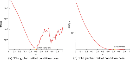
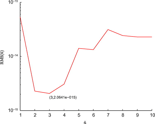
Figure 1(a) displays the RMS error graph of Equation (6.1(6.1) $$\begin{array}{c}\hfill RMS(c)=\sqrt{\frac{1}{N}\sum _{k=1}^N{\left(\frac{{\mathit{\lambda }}_k}{{\left(A^{-1}\right)}_{kk}}\right)}^2},\end{array}$$(6.1) ) with respect to the shape parameter c, for the global initial condition case of Example 1, the optimal value $c^{\ast }$ is 0.49, when the minimum of RMS(c) is $1.17\times {10}^{-5}$. Similarly, Figure 1(b) shows the RMS error graph for the partial initial condition case of Example 1, the optimal value $c^{\ast }$ is 0.72, and the minimum of RMS(c) is $8.13\times {10}^{-2}$, where the variate c locates in the closed interval [0,1]. In Figure 2(b) illustrates the RMS error graph of Equation (3.27(3.27) $$\begin{array}{c}\hfill f(t)=(2\mathit{\nu }-1)\sum _{j=1}^n{p}_j\text{sign}(t-t_j){|t-t_j|}^{2\mathit{\nu }-2}+\sum _{j=1}^{\mathit{\nu }}(j-1)q_j{t}^{j-2}.\end{array}$$(3.27) ) with respect to the integer $\tilde{n}$ of Example 1, the minimum value of RMS($\tilde{n}$) is $1.45\times {10}^{-15}$, and corresponding to ${\tilde{n}}^{\ast }=2$, where $\tilde{n}$ lies in the range of [1,10].

Figure 2. The plots of the exact function u(x, 0) and its approximation (a) with four different noise levels added to the measured data, namely $\mathit{\delta }=0.01\%,\mathit{\delta }=0.1\%,\mathit{\delta }=1\%$ and $\mathit{\delta }=5\%$ for the partial initial condition case, and RMS($\tilde{n}$) (b) with respect to the integer $\tilde{n}$ of Example 1.

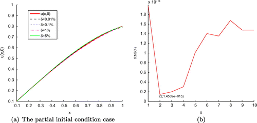
Figure 3. The RMS error (a) of function u(x, t) and its maximum error (b) with $T=1$, and four different noise levels added to the measured data, namely $\mathit{\delta }=0.01\%,\mathit{\delta }=0.1\%,\mathit{\delta }=1\%$ and $\mathit{\delta }=5\%$, for the global initial condition case of Example 1, L denotes time level corresponding to $t=0,0.1,\dots ,1$.

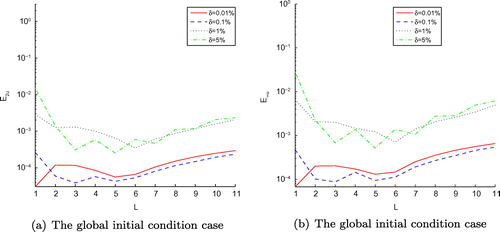
Table 1. The results of $E_{2f}$, $E_{\infty f}$, ${\mathit{\alpha }}_{\text{opt}}(A_0)$ and ${\mathit{\alpha }}_{\text{opt}}(B_0)$ with various error levels, namely $\mathit{\delta }=0.01\%,\mathit{\delta }=0.1\%,\mathit{\delta }=1\%$ and $\mathit{\delta }=5\%$ for the global initial condition case of Example 1.

	$\mathit{\delta }=0.01\%$	$\mathit{\delta }=0.1\%$	$\mathit{\delta }=1\%$	$\mathit{\delta }=5\%$
$E_{2f}$	$8.57\times {10}^{-4}$	$1.25\times {10}^{-3}$	$6.98\times {10}^{-3}$	$8.83\times {10}^{-3}$
$E_{\infty f}$	$1.56\times {10}^{-3}$	$3.01\times {10}^{-3}$	$1.24\times {10}^{-2}$	$1.85\times {10}^{-2}$
${\mathit{\alpha }}_{\text{opt}}(A_0)$	$0.30\times {10}^{-9}$	$0.30\times {10}^{-10}$	$0.30\times {10}^{-6}$	$0.30\times {10}^{-6}$
${\mathit{\alpha }}_{\text{opt}}(B_0)$	$0.80\times {10}^{-9}$	$0.30\times {10}^{-10}$	$0.80\times {10}^{-7}$	$0.80\times {10}^{-8}$

Figure 4. The RMS error (a) of function u(x, t) and its maximum error (b) with $T=1$, and four different noise levels added to the measured data, namely $\mathit{\delta }=0.01\%,\mathit{\delta }=0.1\%,\mathit{\delta }=1\%$ and $\mathit{\delta }=5\%$, for the partial initial condition case of Example 1, L denotes time level corresponding to $t=0,0.1,\dots ,1$.

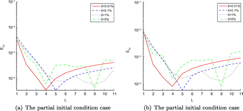
Figure 5. The exact function f(t) and its approximation with four different noise levels added to the measured data, where $\mathit{\delta }=0.01\%,\mathit{\delta }=0.1\%,\mathit{\delta }=1\%$ and $\mathit{\delta }=5\%$ for the global (a) and partial (b) initial condition cases of Example 1.

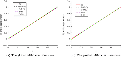
Table 2. The results of $E_{2f}$, $E_{\infty f}$, $E_{2h_2}$, $E_{\infty h_2}$, ${\mathit{\alpha }}_{\text{opt}}(A_0)$ and ${\mathit{\alpha }}_{\text{opt}}(C_0)$ with various error levels, namely $\mathit{\delta }=0.01\%,\mathit{\delta }=0.1\%,\mathit{\delta }=1\%$ and $\mathit{\delta }=5\%$ for the partial initial condition case of Example 1.

	$\mathit{\delta }=0.01\%$	$\mathit{\delta }=0.1\%$	$\mathit{\delta }=1\%$	$\mathit{\delta }=5\%$
$E_{2f}$	$1.69\times {10}^{-3}$	$5.14\times {10}^{-3}$	$4.83\times {10}^{-3}$	$6.43\times {10}^{-3}$
$E_{\infty f}$	$6.07\times {10}^{-3}$	$1.81\times {10}^{-2}$	$1.61\times {10}^{-2}$	$2.00\times {10}^{-2}$
$E_{2h_2}$	$3.52\times {10}^{-3}$	$4.23\times {10}^{-3}$	$3.13\times {10}^{-3}$	$4.89\times {10}^{-3}$
$E_{\infty h_2}$	$8.94\times {10}^{-3}$	$8.40\times {10}^{-3}$	$6.01\times {10}^{-3}$	$8.35\times {10}^{-3}$
${\mathit{\alpha }}_{\text{opt}}(A_0)$	$0.30\times {10}^{-8}$	$0.50\times {10}^{-9}$	$0.50\times {10}^{-10}$	$0.80\times {10}^{-11}$
${\mathit{\alpha }}_{\text{opt}}(C_0)$	$0.90\times {10}^{-6}$	$1.10\times {10}^{-6}$	$0.85\times {10}^{-4}$	$0.22\times {10}^{-3}$

We take consistently the values $h=1/10$ and $\mathit{\tau }={\left(\frac{h}{4}\right)}^2$ for Examples 1–2 in this paper, the over-specification points $x^{\ast }=0.40$ and $x^{\ast }=0.25$ are given for the global and partial initial condition cases of Example 1, respectively, the given data $u_0(x),s(t),l(x)$ and g(t) can be obtained from the exact solution.

Moreover, we can obtain the condition number of interpolation matrices $A_0$ and $B_0$, which can reach ${10}^{13}$ for the global initial condition case, similarly, the condition number of $A_0$ and $C_0$ are equal to ${10}^{17}$, for partial initial condition case of Example 1. The results both RMS error and maximum error of function u(x, t) are shown in Figures 3 and 4, with different time levels $t=0,0.1,\dots ,1$. Figures 5 and 2(a) display the comparison between the exact functions f(t), u(x, 0) and their approximation, with four different noise levels added to the measured data, the numerical results show that our proposed methods are effective and precise.

In Tables 1 and 2, the numerical results are presented for both RMS error and maximum error of f(t), we show that the smaller the noise level $\mathit{\delta }$ chosen is, the better the accuracy of its numerical results is, similar to $h_2(x)$. Moreover, the precision of results obtained is dependent on the regularization parameter chosen. It should be noted that the numerical solutions is quite satisfactory form the Tables above. In addition, to describe clearly, we use the log-scale on the vertical axis for all the figures of Example 1, but except Figures 5 and 2.

Example 2:

Let the exact solution to the problem (3.1(3.1) $$\begin{array}{c}\hfill \frac{\mathit{\partial }u}{\mathit{\partial }t}=\frac{{\mathit{\partial }}^{2}u}{\mathit{\partial }{x}^2}+f(t),0<x<1,0<t\le T,\end{array}$$(3.1) )–(3.4(3.4) $$\begin{array}{c}\hfill u(x^{\ast },t)=g(t),0\le t\le T,\end{array}$$(3.4) ) be [15]:$$\begin{array}{cc}\hfill u(x,t)& =x^2+2t+sin(2\mathit{\pi }t),\hfill \\ \hfill f(t)& =2\mathit{\pi }cos(2\mathit{\pi }t).\hfill \end{array}$$

Figure 6. The plots of RMS(c) with respect to c for two classes of initial condition of Example 2: (a) The global initial condition case, (b) The partial initial condition case.

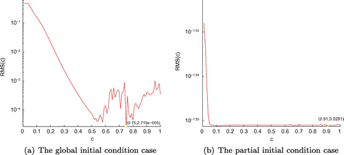
Figure 6(a) displays the RMS error graph of Equation (6.1(6.1) $$\begin{array}{c}\hfill RMS(c)=\sqrt{\frac{1}{N}\sum _{k=1}^N{\left(\frac{{\mathit{\lambda }}_k}{{\left(A^{-1}\right)}_{kk}}\right)}^2},\end{array}$$(6.1) ) with respect to the shape parameter c, for the global initial condition case of Example 2, the optimal value $c^{\ast }$ is 0.75, when the minimum of RMS(c) is $2.72\times {10}^{-5}$. Similarly, Figure 6(b) shows the RMS error graph for the partial initial condition case of Example 2, the optimal value $c^{\ast }$ is 0.91, and the minimum of RMS(c) is $2.81\times {10}^{-2}$, where the variate c locates in the closed interval [0,1]. In Figure 7(b) illustrates the RMS error graph of Equation (3.27(3.27) $$\begin{array}{c}\hfill f(t)=(2\mathit{\nu }-1)\sum _{j=1}^n{p}_j\text{sign}(t-t_j){|t-t_j|}^{2\mathit{\nu }-2}+\sum _{j=1}^{\mathit{\nu }}(j-1)q_j{t}^{j-2}.\end{array}$$(3.27) ) with respect to the integer $\tilde{n}$ of Example 2, the minimum value of RMS($\tilde{n}$) is $9.26\times {10}^{-7}$, and corresponding to ${\tilde{n}}^{\ast }=4$, where $\tilde{n}$ lies in the range of [1,10].

Figure 7. The plots of the exact function u(x, 0) and its approximation (a) with four different noise levels added to the measured data, namely $\mathit{\delta }=0.02\%,\mathit{\delta }=0.2\%,\mathit{\delta }=1\%$ and $\mathit{\delta }=5\%$ for the partial initial condition case, and RMS($\tilde{n}$) (b) with respect to the integer $\tilde{n}$ of Example 2.

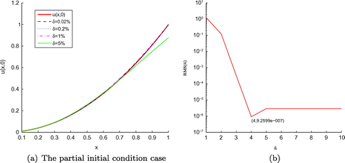
Figure 8. The plots of the exact f(t) and its approximation function to see literature [15] in Example 2.

Figure 9. The exact function f(t) and its approximation with four different noise levels added to the measured data, namely $\mathit{\delta }=0.01\%,\mathit{\delta }=0.1\%,\mathit{\delta }=1\%$ and $\mathit{\delta }=5\%$ for the global (a) initial condition case of Example 2 , and the partial (b) initial condition case with $\mathit{\delta }=0.02\%,\mathit{\delta }=0.2\%,\mathit{\delta }=1\%$ and $\mathit{\delta }=5\%$, respectively.

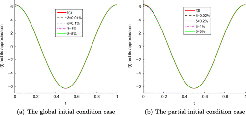
Table 3. The results of $E_{2f}$, $E_{\infty f}$, ${\mathit{\alpha }}_{\text{opt}}(A_0)$ and ${\mathit{\alpha }}_{\text{opt}}(B_0)$ with various error levels, $\mathit{\delta }=0.01\%,\mathit{\delta }=0.1\%,\mathit{\delta }=1\%$ and $\mathit{\delta }=5\%$ for the global initial condition case of Example 2.

	$\mathit{\delta }=0.01\%$	$\mathit{\delta }=0.1\%$	$\mathit{\delta }=1\%$	$\mathit{\delta }=5\%$
$E_{2f}$	$1.74\times {10}^{-3}$	$1.81\times {10}^{-3}$	$7.09\times {10}^{-3}$	$9.89\times {10}^{-3}$
$E_{\infty f}$	$1.18\times {10}^{-2}$	$1.43\times {10}^{-2}$	$5.28\times {10}^{-2}$	$8.85\times {10}^{-2}$
${\mathit{\alpha }}_{\text{opt}}(A_0)$	$0.30\times {10}^{-9}$	$0.30\times {10}^{-9}$	$0.30\times {10}^{-10}$	$0.50\times {10}^{-9}$
${\mathit{\alpha }}_{\text{opt}}(B_0)$	$0.40\times {10}^{-10}$	$0.30\times {10}^{-9}$	$0.30\times {10}^{-10}$	$0.30\times {10}^{-9}$

Figure 10. The RMS error (a) of function u(x, t) and its maximum error (b) with $T=1$, and four noise levels added to the measured data, namely $\mathit{\delta }=0.01\%,\mathit{\delta }=0.1\%,\mathit{\delta }=1\%$ and $\mathit{\delta }=5\%$, for the global initial condition case of Example 2, L denotes time level corresponding to $t=0,0.1,\dots ,1$.

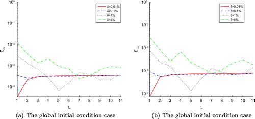
Figure 11. The RMS error (a) of function u(x, t) and its maximum error (b) with $T=1$, with four different noise levels added to the measured data, namely $\mathit{\delta }=0.02\%,\mathit{\delta }=0.2\%,\mathit{\delta }=1\%$ and $\mathit{\delta }=5\%$, for the partial initial condition case of Example 2, L denotes time level corresponding to $t=0,0.1,\dots ,1$.

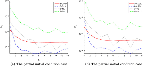
Table 4. The results of $E_{2f}$, $E_{\infty f}$, $E_{2h_2}$, $E_{\infty h_2}$, ${\mathit{\alpha }}_{\text{opt}}(A_0)$ and ${\mathit{\alpha }}_{\text{opt}}(C_0)$ with various error levels, namely $\mathit{\delta }=0.02\%,\mathit{\delta }=0.2\%,\mathit{\delta }=1\%$ and $\mathit{\delta }=5\%$ for the partial initial condition case of Example 2.

	$\mathit{\delta }=0.02\%$	$\mathit{\delta }=0.2\%$	$\mathit{\delta }=1\%$	$\mathit{\delta }=5\%$
$E_{2f}$	$3.64\times {10}^{-3}$	$5.23\times {10}^{-3}$	$9.36\times {10}^{-3}$	$3.30\times {10}^{-2}$
$E_{\infty f}$	$1.55\times {10}^{-2}$	$2.88\times {10}^{-2}$	$5.68\times {10}^{-2}$	$1.87\times {10}^{-1}$
$E_{2h_2}$	$1.42\times {10}^{-3}$	$3.04\times {10}^{-3}$	$4.59\times {10}^{-3}$	$4.20\times {10}^{-2}$
$E_{\infty h_2}$	$2.67\times {10}^{-3}$	$8.31\times {10}^{-3}$	$8.78\times {10}^{-3}$	$1.23\times {10}^{-1}$
${\mathit{\alpha }}_{\text{opt}}(A_0)$	$0.50\times {10}^{-10}$	$0.80\times {10}^{-11}$	$0.50\times {10}^{-11}$	$0.80\times {10}^{-11}$
${\mathit{\alpha }}_{\text{opt}}(C_0)$	$0.16\times {10}^{-8}$	$0.75\times {10}^{-7}$	$0.27\times {10}^{-6}$	$0.14\times {10}^{-3}$

We take the over-specification point $x^{\ast }=0.25$ for the global and partial initial condition cases of Example 2. Furthermore, we can obtain the condition numbers of the interpolation matrices $A_0$, $B_0$ and $C_0$ which lie in the range of ${10}^{17}\text{--}{10}^{18}$, for the global and partial initial cases of Example 2. Specially, the two plots of the exact f(t) and its approximation, addressed in Figure 8 by Xiong et al. [15], are oscillatory and fluctuant, but the pictures obtained by our proposed method in Figures 9(a) and (b) are stable and satisfactory. In Figure 7(a), we show that the plot of both the exact function u(x, 0) and its approximation with four different noise levels, the numerical results of the last noise level, i.e. $\mathit{\delta }=5\%$, are not as good as ones of the first three kinds cases. We should note that the accuracy of function u(x, 0) depend on the number of data points, the chosen noise levels, the regularization parameters ${\mathit{\alpha }}_{\text{opt}}(·)$ selected and the optimal shape parameter $c^{\ast }$ according to different numerical results above. From Figures 10 and 11, Tables 3–4, our proposed methods are quite effective to solve the IHCP. In addition, we use the log-scale on the vertical axis for all the figures of Example 2, but except Figures 7–9.

Example 3:

In this example, we give a two-dimensional case with the exact solution to the problem (4.1(4.1) $$\begin{array}{c}\hfill \frac{\mathit{\partial }u}{\mathit{\partial }t}=\frac{{\mathit{\partial }}^{2}u}{\mathit{\partial }{x}^2}+\frac{{\mathit{\partial }}^{2}u}{\mathit{\partial }{y}^2}+f(t),0<x<1,0<y<1,0<t\le T,\end{array}$$(4.1) )–(4.5(4.5) $$\begin{array}{c}\hfill u(x^{\ast },y^{\ast },t)=g(t),0\le t\le T,\end{array}$$(4.5) ) as:$$\begin{array}{cc}\hfill u(x,y,t)& =exp(-t)(sinx+cosy)+t^2-\frac{t^3}{2},\hfill \\ \hfill f(t)& =2t-\frac{3t^2}{2}.\hfill \end{array}$$

In order to demonstrate the superiority of the proposed method for the given problems with other methods, in the term of computation time and accuracy, we compare with the numerical results of MFS devised by Wen [12] (called MFS) in Example 3, with regular rectangular domain and non-rectangular domain (such as the Circular-domain, the Peanut-domain), respectively. CPU(s) denotes the amount time for processing instructions of a computer program, and the time unit is defined in second (s). There are several parameters need to be determined in both our algorithms and MFS, we only compute the total time of algorithms with respect to CPU(s), but not to include the computation cost for selecting those parameters to two schemes above in this paper. All the programs are running in Intel’s Core I7-3520M CPU @ 2.90GHz.

6.1. Example 3-1 For the rectangular domain

Figure 12. The plot of RMS($\tilde{n}$) with respect to $\tilde{n}$ of Example 3 for the rectangular domain.

Figure 13. The plots of RMS(c) with respect to c for two classes of initial condition of Example 3 for the rectangular domain: (a) The global initial condition case, (b) The partial initial condition case.

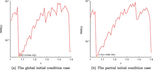
In Figure 12, the plot shows the RMS error of Equation (3.27(3.27) $$\begin{array}{c}\hfill f(t)=(2\mathit{\nu }-1)\sum _{j=1}^n{p}_j\text{sign}(t-t_j){|t-t_j|}^{2\mathit{\nu }-2}+\sum _{j=1}^{\mathit{\nu }}(j-1)q_j{t}^{j-2}.\end{array}$$(3.27) ) with respect to the integer $\tilde{n}$ of Example 3 for the rectangular domain, the minimum value of RMS($\tilde{n}$) is $2.06\times {10}^{-15}$, and corresponding to ${\tilde{n}}^{\ast }=3$, where $\tilde{n}$ lies in the range of [1,10]. Figure 13(a) displays the RMS error graph of Equation (6.1(6.1) $$\begin{array}{c}\hfill RMS(c)=\sqrt{\frac{1}{N}\sum _{k=1}^N{\left(\frac{{\mathit{\lambda }}_k}{{\left(A^{-1}\right)}_{kk}}\right)}^2},\end{array}$$(6.1) ) with respect to the shape parameter c, for the global initial condition case of Example 3, the optimal value $c^{\ast }$ is 1.07, when the minimum value of RMS(c) is $3.68\times {10}^{-5}$. Similarly, Figure 13(b) shows the RMS error graph for the partial initial condition case of Example 3, the optimal value $c^{\ast }$ is 1.05, and the minimum value of RMS(c) is $4.10\times {10}^{-5}$, where the variate c locates in the close interval [1,1.5].

Figure 14. The exact function f(t) and its approximation with four different noise levels added to the measured data, namely $\mathit{\delta }=0.01\%,\mathit{\delta }=0.1\%,\mathit{\delta }=1\%$ and $\mathit{\delta }=5\%$, for the global (Ours) (a) and global (MFS) (b) initial condition cases of Example 3 for the rectangular domain, respectively.

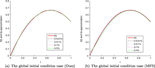
Figure 15. The exact function f(t) and its approximation with four different noise levels added to the measured data, namely $\mathit{\delta }=0.01\%,\mathit{\delta }=0.1\%,\mathit{\delta }=1\%$ and $\mathit{\delta }=5\%$, for the partial (Ours) (a) and partial (MFS) (b) initial condition cases of Example 3 for the rectangular domain, respectively.

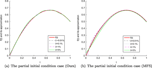
Figure 16. The RMS error (a) of function u(x, y, t) and its maximum error (b) obtained by our proposed scheme with $T=1$, and four different noise levels added to the measured data, namely $\mathit{\delta }=0.01\%,\mathit{\delta }=0.1\%,\mathit{\delta }=1\%$ and $\mathit{\delta }=5\%$, for the global initial condition case of Example 3 for the rectangular domain, L denotes time level corresponding to $t=0,0.1,\dots ,1$.

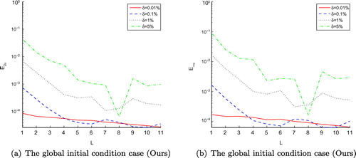
Table 5. The results of $E_{2f}$, $E_{\infty f}$, CPU(s) obtained by our technique and MFS with various error levels, $\mathit{\delta }=0.01\%,\mathit{\delta }=0.1\%,\mathit{\delta }=1\%$ and $\mathit{\delta }=5\%$ for the global initial condition case of Example 3 for the rectangular domain.

		$\mathit{\delta }=0.01\%$	$\mathit{\delta }=0.1\%$	$\mathit{\delta }=1\%$	$\mathit{\delta }=5\%$
	$E_{2f}$	$1.07\times {10}^{-3}$	$1.61\times {10}^{-3}$	$2.46\times {10}^{-3}$	$1.04\times {10}^{-2}$
Ours	$E_{\infty f}$	$3.63\times {10}^{-3}$	$4.64\times {10}^{-3}$	$9.31\times {10}^{-3}$	$3.53\times {10}^{-2}$
	CPU(s)	19.92	19.90	19.99	19.87
	$E_{2f}$	$8.92\times {10}^{-4}$	$1.92\times {10}^{-3}$	$6.71\times {10}^{-3}$	$1.44\times {10}^{-2}$
MFS	$E_{\infty f}$	$2.55\times {10}^{-3}$	$1.03\times {10}^{-2}$	$4.47\times {10}^{-2}$	$4.99\times {10}^{-2}$
	CPU(s)	35.75	35.94	37.00	36.86

Figure 17. The RMS error (a) of function u(x, y, t) and its maximum error (b) obtained by MFS with $T=1$, and four different noise levels added to the measured data, namely $\mathit{\delta }=0.01\%,\mathit{\delta }=0.1\%,\mathit{\delta }=1\%$ and $\mathit{\delta }=5\%$, for the global initial condition case of Example 3 for the rectangular domain, L denotes time level corresponding to $t=0,0.1,\dots ,1$.

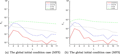
Figure 18. The RMS error (a) of function u(x, y, t) and its maximum error (b) obtained by our method with $T=1$, with four different noise levels added to the measured data, namely $\mathit{\delta }=0.01\%,\mathit{\delta }=0.1\%,\mathit{\delta }=1\%$ and $\mathit{\delta }=5\%$, for the partial initial condition case of Example 3 for the rectangular domain, L denotes time level corresponding to $t=0,0.1,\dots ,1$.

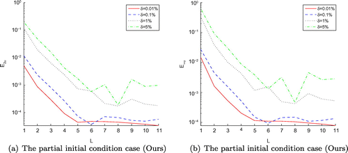
Figure 19. The RMS error (a) of function u(x, y, t) and its maximum error (b) obtained by MFS with $T=1$, with four different noise levels added to the measured data, namely $\mathit{\delta }=0.01\%,\mathit{\delta }=0.1\%,\mathit{\delta }=1\%$ and $\mathit{\delta }=5\%$, for the partial initial condition case of Example 3 for the rectangular domain, L denotes time level corresponding to $t=0,0.1,\dots ,1$.

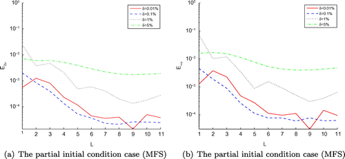
Table 6. The results of $E_{2f}$, $E_{\infty f}$, $E_{2h_2}$, $E_{\infty h_2}$, CPU(s) obtained by our technique and MFS with various error levels, namely $\mathit{\delta }=0.01\%,\mathit{\delta }=0.1\%,\mathit{\delta }=1\%$ and $\mathit{\delta }=5\%$ for the partial initial condition case of Example 3 for the rectangular domain.

		$\mathit{\delta }=0.01\%$	$\mathit{\delta }=0.1\%$	$\mathit{\delta }=1\%$	$\mathit{\delta }=5\%$
	$E_{2f}$	$1.42\times {10}^{-3}$	$1.49\times {10}^{-3}$	$1.58\times {10}^{-3}$	$6.47\times {10}^{-3}$
	$E_{\infty f}$	$2.91\times {10}^{-3}$	$3.18\times {10}^{-3}$	$4.13\times {10}^{-3}$	$1.50\times {10}^{-2}$
Ours	$E_{2h_2}$	$5.06\times {10}^{-3}$	$1.17\times {10}^{-2}$	$1.16\times {10}^{-1}$	$1.95\times {10}^{-1}$
	$E_{\infty h_2}$	$1.50\times {10}^{-2}$	$2.74\times {10}^{-2}$	$3.35\times {10}^{-1}$	$6.29\times {10}^{-1}$
	CPU(s)	20.22	20.15	21.87	21.38
	$E_{2f}$	$4.48\times {10}^{-3}$	$3.41\times {10}^{-3}$	$2.58\times {10}^{-2}$	$1.58\times {10}^{-2}$
	$E_{\infty f}$	$1.32\times {10}^{-2}$	$2.87\times {10}^{-2}$	$1.95\times {10}^{-1}$	$4.39\times {10}^{-2}$
MFS	$E_{2h_2}$	$5.52\times {10}^{-4}$	$2.56\times {10}^{-3}$	$2.70\times {10}^{-2}$	$1.02\times {10}^{-2}$
	$E_{\infty h_2}$	$1.32\times {10}^{-2}$	$5.50\times {10}^{-3}$	$7.75\times {10}^{-2}$	$3.05\times {10}^{-2}$
	CPU(s)	37.21	36.92	36.99	36.86

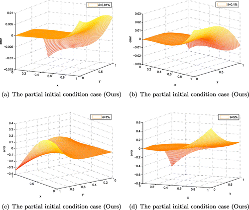
Figure 20. The error plots between the exact function u(x, y, 0) and its approximation $\tilde{u}(x,y,0)$ obtained by our method with $T=1$, with four different noise levels added to the measured data, namely $\mathit{\delta }=0.01\%,\mathit{\delta }=0.1\%,\mathit{\delta }=1\%$ and $\mathit{\delta }=5\%$ for the partial initial condition case of Example 3 for the rectangular domain.

We consistently take the values $x^{\ast }=y^{\ast }=0.5$, $\mathrm{\Delta }x=\mathrm{\Delta }y=1/5$ and $\mathit{\tau }={\left(\frac{h}{4}\right)}^2$ in the rectangular domain of Example 3 for the rectangular domain case, the given data $\mathit{\phi }(x,y),f_1(y,t),f_2(x,t),f_3(y,t)$ and $f_4(x,t)$ can be computed from the exact solution. Moreover, the condition numbers of matrices $A_1,B_1$ and $C_1$ lie in the range of ${10}^{16}--{10}^{17}$. In Figures 14 and 15, the numerical results obtained from the noise level $\mathit{\delta }=5\%$ are not as accurate as others, it means that the stability of numerical algorithm proposed is affected by noise level chosen, if the bigger noise level is selected, the numerical results are shown to be more inaccurate in the test experiments. Furthermore, our provided methods are quite satisfactory and need less computation time than MFS according to the Figures 16–17, 18–20 and Tables 5–6. Additionally, in order to describe clearly, we use the log-scale on the vertical axis for all the figures of Example 3, but except Figures 14–15 and 20. It should be noted that the regularization parameters ${\mathit{\alpha }}_{\text{opt}}(·)$ chosen in all examples above are concerned with the noise level $\mathit{\delta }$ desired, if the smaller value of noise level is given, the influence on computational accuracy is little to choose from a wide range of the parameter ${\mathit{\alpha }}_{\text{opt}}(·)$. Otherwise, if a larger noise level is desired, the numerical results are very sensitive to the regularization parameter selected, and sometimes no matter how to choose a regularization parameter, it is impossible to get a satisfactory approximation.

6.2. Example 3-2 For the non-rectangular domain

In this part, we develop two types non-rectangular domain, such as the Circular-domain and the Peanut-domain, respectively, to discuss the given 2-D IHCPs with the Neumann boundary condition. In such a setting, we replace the domain $\mathrm{\Omega }=\{(x,y,t):0\le x,y\le 1,0\le t\le T\}$ of Equations (4.1(4.1) $$\begin{array}{c}\hfill \frac{\mathit{\partial }u}{\mathit{\partial }t}=\frac{{\mathit{\partial }}^{2}u}{\mathit{\partial }{x}^2}+\frac{{\mathit{\partial }}^{2}u}{\mathit{\partial }{y}^2}+f(t),0<x<1,0<y<1,0<t\le T,\end{array}$$(4.1) )–(4.5(4.5) $$\begin{array}{c}\hfill u(x^{\ast },y^{\ast },t)=g(t),0\le t\le T,\end{array}$$(4.5) ) by the following Circular-domain(6.4) $$\begin{array}{c}\hfill \mathit{\partial }\mathrm{\Omega }=\{(x,y,t):x=\mathit{\rho }cos(\mathit{\theta }),y=\mathit{\rho }sin(\mathit{\theta }),0\le t\le T,\mathit{\rho }>0,-\mathit{\pi }\le \mathit{\theta }\le \mathit{\pi }\},\end{array}$$(6.4)

or the following Peanut-domain(6.5) $$\begin{array}{c}\hfill \mathit{\partial }\mathrm{\Omega }=\{(x,y,t):x=\mathit{\rho }(\mathit{\theta })cos(\mathit{\theta }),y=\mathit{\rho }(\mathit{\theta })sin(\mathit{\theta }),0\le t\le T,-\mathit{\pi }\le \mathit{\theta }\le \mathit{\pi }\},\end{array}$$(6.5)

where$$\begin{array}{c}\hfill \mathit{\rho }(\mathit{\theta })={\left(cos(2\mathit{\theta })+\sqrt{1.1-{sin}^2(2\mathit{\theta })}\right)}^{\frac{1}{2}}.\end{array}$$

The Neumann boundary conditions (4.3(4.3) $$\begin{array}{c}\hfill u_x(0,y,t)=f_1(y,t),u_x(1,y,t)=f_3(y,t),0\le y\le 1,0\le t\le T,\end{array}$$(4.3) )–(4.4(4.4) $$\begin{array}{c}\hfill u_y(x,0,t)=f_2(x,t),u_y(x,1,t)=f_4(x,t),0\le x\le 1,0\le t\le T,\end{array}$$(4.4) ) are defined again as follows(6.6) $$\begin{array}{c}\hfill \frac{\mathit{\partial }u}{\mathit{\partial }\overrightarrow{n}}=u_N,\text{on}\mathit{\partial }\mathrm{\Omega },\end{array}$$(6.6)

where $\mathit{\partial }\mathrm{\Omega }$ is boundary of the bounded domain $\mathrm{\Omega }$, $\overrightarrow{n}$ is the outer unit normal with respect to $\mathit{\partial }\mathrm{\Omega }$, $u_N$ is the known and measured Neumann data, but the remaining Equations (4.1(4.1) $$\begin{array}{c}\hfill \frac{\mathit{\partial }u}{\mathit{\partial }t}=\frac{{\mathit{\partial }}^{2}u}{\mathit{\partial }{x}^2}+\frac{{\mathit{\partial }}^{2}u}{\mathit{\partial }{y}^2}+f(t),0<x<1,0<y<1,0<t\le T,\end{array}$$(4.1) ), (4.2(4.2) $$\begin{array}{c}\hfill u(x,y,0)=\mathit{\phi }(x,y),0\le x\le 1,0\le y\le 1,\end{array}$$(4.2) ) and (4.5(4.5) $$\begin{array}{c}\hfill u(x^{\ast },y^{\ast },t)=g(t),0\le t\le T,\end{array}$$(4.5) ) are unchanged. Without loss of generality, we employ the same exact solution of Example 3 for the Circular-domain and Peanut-domain to discuss the numerical results of the proposed method and MFS.

Figure 21. The exact function f(t) and its approximation with four different noise levels added to the measured data, namely $\mathit{\delta }=0.01\%,\mathit{\delta }=0.1\%,\mathit{\delta }=1\%$ and $\mathit{\delta }=5\%$, for the global (Ours) (a) and global (MFS) (b) initial condition cases of Example 3 in the Circular-domain setting, respectively.

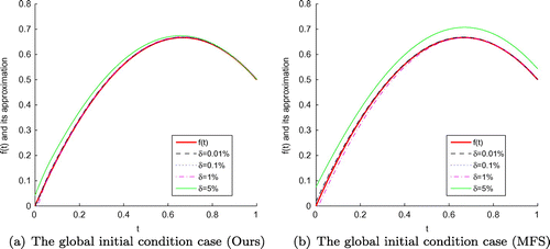
Figure 22. The exact function f(t) and its approximation with four different noise levels added to the measured data, namely $\mathit{\delta }=0.01\%,\mathit{\delta }=0.1\%,\mathit{\delta }=1\%$ and $\mathit{\delta }=5\%$, for the partial (Ours) (a) and partial (MFS) (b) initial condition cases of Example 3 in the Peanut-domain setting, respectively.

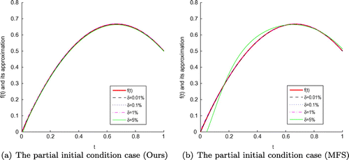
Figure 23. The Circular-domain (a) and the Peanut-domain (b), and the notation "+" denotes the chosen collocation point.

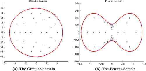
Figure 24. The RMS error (a) of function u(x, y, t) and its maximum error (b) obtained by our proposed scheme with $T=1$, and four different noise levels added to the measured data, namely $\mathit{\delta }=0.01\%,\mathit{\delta }=0.1\%,\mathit{\delta }=1\%$ and $\mathit{\delta }=5\%$, for the global initial condition case of Example 3 in the Circular-domain setting, L denotes time level corresponding to $t=0,0.1,\dots ,1$.

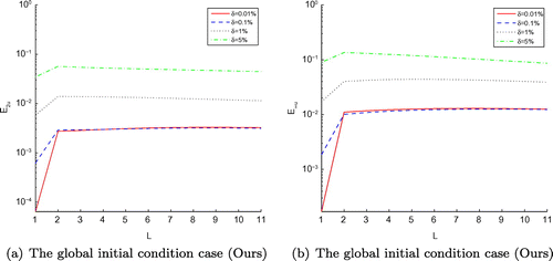
Table 7. The results of $E_{2f}$, $E_{\infty f}$, CPU(s) obtained by our technique and MFS with various error levels, $\mathit{\delta }=0.01\%,\mathit{\delta }=0.1\%,\mathit{\delta }=1\%$ and $\mathit{\delta }=5\%$ for the global initial condition case of Example 3 in the Circular-domain setting.

		$\mathit{\delta }=0.01\%$	$\mathit{\delta }=0.1\%$	$\mathit{\delta }=1\%$	$\mathit{\delta }=5\%$
	$E_{2f}$	$3.18\times {10}^{-3}$	$3.72\times {10}^{-3}$	$5.11\times {10}^{-3}$	$2.33\times {10}^{-2}$
Ours	$E_{\infty f}$	$7.34\times {10}^{-3}$	$2.02\times {10}^{-2}$	$3.61\times {10}^{-2}$	$4.90\times {10}^{-2}$
	CPU(s)	39.84	35.89	34.59	35.45
	$E_{2f}$	$5.56\times {10}^{-3}$	$4.17\times {10}^{-3}$	$1.16\times {10}^{-2}$	$4.41\times {10}^{-2}$
MFS	$E_{\infty f}$	$1.76\times {10}^{-2}$	$1.43\times {10}^{-2}$	$2.24\times {10}^{-2}$	$7.54\times {10}^{-2}$
	CPU(s)	72.63	67.24	67.00	66.63

Figure 25. The RMS error (a) of function u(x, y, t) and its maximum error (b) obtained by MFS with $T=1$, and four different noise levels added to the measured data, namely $\mathit{\delta }=0.01\%,\mathit{\delta }=0.1\%,\mathit{\delta }=1\%$ and $\mathit{\delta }=5\%$, for the global initial condition case of Example 3 in the Circular-domain setting, L denotes time level corresponding to $t=0,0.1,\dots ,1$.

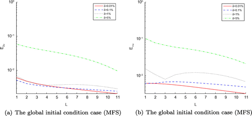
Figure 26. The RMS error (a) of function u(x, y, t) and its maximum error (b) obtained by our method with $T=1$, and four different noise levels added to the measured data, namely $\mathit{\delta }=0.01\%,\mathit{\delta }=0.1\%,\mathit{\delta }=1\%$ and $\mathit{\delta }=5\%$, for the partial initial condition case of Example 3 in the Peanut-domain setting, L denotes time level corresponding to $t=0,0.1,\dots ,1$.

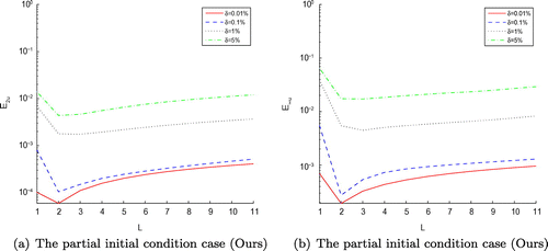
Figure 27. The RMS error (a) of function u(x, y, t) and its maximum error (b) obtained by MFS with $T=1$, and four different noise levels added to the measured data, namely $\mathit{\delta }=0.01\%,\mathit{\delta }=0.1\%,\mathit{\delta }=1\%$ and $\mathit{\delta }=5\%$, for the partial initial condition case of Example 3 in the Peanut-domain setting, L denotes time level corresponding to $t=0,0.1,\dots ,1$.

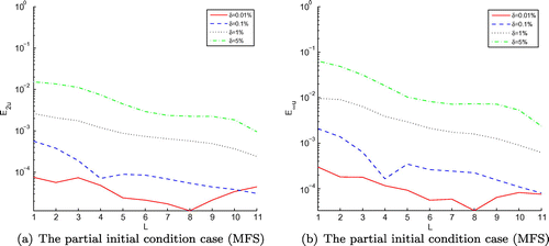
Table 8. The results of $E_{2f}$, $E_{\infty f}$, $E_{2h_2}$, $E_{\infty h_2}$, CPU(s) obtained by our technique and MFS with various error levels, namely $\mathit{\delta }=0.01\%,\mathit{\delta }=0.1\%,\mathit{\delta }=1\%$ and $\mathit{\delta }=5\%$ for the partial initial condition case of Example 3 in the Peanut-domain setting.

		$\mathit{\delta }=0.01\%$	$\mathit{\delta }=0.1\%$	$\mathit{\delta }=1\%$	$\mathit{\delta }=5\%$
	$E_{2f}$	$6.34\times {10}^{-4}$	$1.81\times {10}^{-3}$	$3.81\times {10}^{-3}$	$4.46\times {10}^{-3}$
	$E_{\infty f}$	$1.47\times {10}^{-3}$	$3.55\times {10}^{-3}$	$1.00\times {10}^{-2}$	$1.85\times {10}^{-2}$
Ours	$E_{2h_2}$	$1.08\times {10}^{-4}$	$8.45\times {10}^{-4}$	$7.24\times {10}^{-3}$	$1.61\times {10}^{-2}$
	$E_{\infty h_2}$	$9.65\times {10}^{-4}$	$5.55\times {10}^{-3}$	$3.90\times {10}^{-2}$	$6.48\times {10}^{-2}$
	CPU(s)	36.25	39.72	35.77	35.97
	$E_{2f}$	$2.04\times {10}^{-4}$	$1.39\times {10}^{-3}$	$2.81\times {10}^{-3}$	$3.11\times {10}^{-2}$
	$E_{\infty f}$	$7.11\times {10}^{-4}$	$9.19\times {10}^{-3}$	$1.09\times {10}^{-2}$	$8.83\times {10}^{-2}$
MFS	$E_{2h_2}$	$7.58\times {10}^{-5}$	$5.66\times {10}^{-4}$	$2.62\times {10}^{-3}$	$1.54\times {10}^{-2}$
	$E_{\infty h_2}$	$3.30\times {10}^{-4}$	$2.11\times {10}^{-3}$	$9.70\times {10}^{-3}$	$6.38\times {10}^{-2}$
	CPU(s)	71.59	71.85	71.55	70.73

We entirely take 53 collocation points in the Circular-domain and Peanut-domain settings of Example 3 for two different types initial conditions, and the radius $\mathit{\rho }=5$, the over-specification data $x^{\ast }=5cos(\frac{\mathit{\pi }}{3})$, $y^{\ast }=5sin(\frac{\mathit{\pi }}{3})$ for the Circular-domain case, analogously, $x^{\ast }=\mathit{\rho }(\frac{\mathit{\pi }}{3})cos(\frac{\mathit{\pi }}{3})$, $y^{\ast }=\mathit{\rho }(\frac{\mathit{\pi }}{3})sin(\frac{\mathit{\pi }}{3})$ for the Peanut-domain case, respectively. According to the numerical results obtained by our developed schemes and MFS, it is shown that the numerical simulation of function f(t) reconstructed by our techniques is better and stabler, especially, when the noise level becomes larger, the final results acquired by our method are more accurate by Figures 14, 15, 21–26. In addition, the cost time of CPU desired by MFS requires almost 2 times than our schemes do by Tables 5–8.

7. Conclusions

In this paper, a numerical recursion scheme constructed by the Gaussian RBFs method is used for solving a class of inverse parabolic problems, with time-dependent heat source f(t). Our proposed methods adopt the time and space variables separation techniques to approximate the solutions of given problems, which is more suitable for physical meaning to the heat conduction diffusion equations. Comparing with the global collocation points method demonstrated in [12,13], we require only little collocation points in spatial-domain to reconstruct the approximation function, thus, a system of linear equations generated is smaller than that presented in [12,13]. The several parameters (such as, the GCV parameter ${\mathit{\alpha }}_{\text{opt}}$ in Equation (2.11(2.11) $$\begin{array}{c}\hfill {\mathit{\alpha }}_{\text{opt}}=\underset{\mathit{\alpha }\in {\mathbb{R}}^{+}}{\text{argmin}}G(\mathit{\alpha }),\end{array}$$(2.11) ), the regularization parameter ${\tilde{n}}^{\ast }$ in Equation (3.22(3.22) $$\begin{array}{c}\hfill \tilde{M}z=\tilde{b}\end{array}$$(3.22) ) and the shape parameter $c^{\ast }$ in Equation (6.2(6.2) $$\begin{array}{c}\hfill c^{\ast }={\text{argmin}}_{c>0}RMS(c).\end{array}$$(6.2) )) are required to select in this paper, thus, the total computational cost may be a little long, we will improve this in our further work. Overall, we present four numerical algorithms to compute the one-dimensional and two-dimensional initial condition cases, the numerical results are given to show that our proposed schemes are very satisfactory and effective, including the non-rectangular domain.

Additional information

Funding

This work was supported by the National Natural Science Foundation of China [grant numbers 11471066 and 11290143]; the Fundamental Research of Civil Aircraft [grant number MJ-F-2012-04]; the Fundamental Research Funds for the Central Universities [DUT15LK44], and the Scientific Research Funds of Inner Mongolia University for the Nationalities [NMD1304].

Notes

No potential conflict of interest was reported by the authors.

References

- Hào DN, Thanh PX, Lesnic D, et al. A boundary element method for multi-dimensional inverse heat conduction problem. Int. J. Comput. Math. 2012;89:1540–1554.
- Hon YC, Wei T. A fundamental solution method for inverse heat conduction problem. Eng. Anal. Bound. Elem. 2004;28:489–495.
- Fasshauer GE. Meshfree approximation methods with matlab. London: Word Scientific; 2007.
- Ramachandran PA. Method of fundamental solution: singular value decomposition analysis. Commun. Numer. Methods Eng. 2002;18:789–801.
- Tatari M, Dehghan M. A method for solving partial differential equations via radial basis functions: Application to the heat equation. Eng. Anal. Bound. Elem. 2010;34:206–212.
- Dehghan M. Numerical solution of one-dimensional parabolic inverse problem. Appl. Math. Comput. 2003;136:333–344.
- Dehghan M. Finding a control parameter in one-dimensional parabolic equations. Appl. Math. Comput. 2003;135:491–503.
- Dehghan M. An inverse problem of finding a source parameter in a semilinear parabolic equation. Appl. Math. Model. 2001;25:743–754.
- Dehghan M. Parameter determination in a partial differential equation from the overspecified data. Math. Comput. Model. 2005;41:197–213.
- Hon YC, Wei T. The method of fundamental solution for solving multidimensional inverse heat conduction problems. CMES. Comput. Model. Eng. Sci. 2005;7:119–132.
- Dong CF, Sun FY, Meng BQ. A method of fundamental solutions for inverse heat conduction problems in an anisotropic medium. Eng. Anal. Bound. Elem. 2007;31:75–82.
- Wen J. A meshless method for reconstructing the heat source and partial initial temperature in heat conduction. Inverse Probl. Sci. Eng. 2011;21:1007–1022.
- Wen J, Yamamoto M, Wei T. Simultaneous determination of a time-dependent heat source and the initial temperature in an inverse heat conduction problem. Inverse Probl. Sci. Eng. 2013;21:485–499.
- Yan L, Fu CL, Yang FL. The method of fundamental solutions for the inverse heat source problem. Eng. Anal. Bound. Elem. 2008;32:216–222.
- Xiong XT, Yan YM, Wang JX. A direct numerical method for solving inverse heat source problems. J. Phys.: Conf. Ser. 2011;290:012017
- Dehghan M, Tatari M. Determination of a control parameter in a one-dimensional parabolic equation using the method of radial basis functions. Math. Comput. Model. 2006;44:1160–1168.
- Dehghan M. Fourth-order techniques for identifying a control parameter in the parabolic equations. Int. J. Eng. Sci. 2002;40:433–447.
- Dehghan M, Shakeri F. Method of lines solutions of the parabolic inverse problem with an overspecification at a point. Numer. Algorithms. 2009;50:417–437.
- Saadatmandi A, Dehghan M. Computation of two time-dependent coefficients in a parabolic partial differential equation subject to additional specifications. Int. J. Comput. Math. 2010;87:997–1008.
- Lakestani M, Dehghan M. The use of Chebyshev cardinal functions for the solution of a partial differetial equation with an unknown time-dependent coefficient subject to an extra measurement. J. Comput. Appl. Math. 2010;87:997–1008.
- Ma LM, Wu ZM. Radial basis functions method for parabolic inverse problem. Int. J. Comput. Math. 2011;88:384–395.
- Dehghan M, Abbaszadeh M, Mohebbi A. The numerical solution of nonlinear high dimensional generalized Benjamin-Bona-Mahony-Burgers equation via the meshless method of radial basis function. Comput. Math. Appl. 2014;68:212–237.
- Dehghan M, Mohammadi V. The numerical solution of Cahn-Hilliard (CH) equation in one, two and three-dimensions via globally radial basis functions (GRBFs) and RBFs-differential quadrature (RBFs-DQ) methods. Eng. Anal. Bound. Elem. 2015;51:74–100.
- Buhmann MD. Radial basis functions: theory and implementations. Cambridge: Cambridge University Press; 2003.
- Schoenberg IJ. Metrc spaces and completely monotone functions. Ann. Math. 1938:811–841.
- Rippa S. An algorithm for selecting a good value for the parameter c in radial basis function interpolation. Adv. Comput. Math. 1999;11:193–210.
- Hadamard J. Lectures on Cauchy’s problem in linear partial differential equations. New Haven: Yale University Press; 1923.
- Hansen PC. Regularization tools: a Matlab package for analysis and solution of discrete ill-posed problems. Numer. Algorithms. 1994;6:1–35.
- Björck Å. Numerical Method for Least Squares Problems. Philadelphia: SIAM; 1996.
- Golub GH, Loan CFV. Matrix computations. 3rd ed. Baltimore: Johns Hopkins; 1996.
- Tikhonov AN, Arsenin VY. Solutions of ill-posed problems. Washington (DC), New York (NY): V.H. Winston & Sons, John Wiley & Sons; 1977.
- Craven P, Wahba G. Smoothing noisy data with spline functions. Numer. Math. 1979;31:377–403.
- Goulb GH, Heath M, Wahba G. Generalized cross-Validation as a method for choosing a good ridge parameter. Technometrics. 1979;21:215–223.
- Wahba G, Wendelberger J. Some new mathematical methods for variational objective analysis using splines and cross validation. Monthly Weather Rev. 1980;108:1122–1143.
- Hanke M, Scherzer O. Inverse problems light: numerical differentiation. Am. Math. Mon. 2001;108:512–521.
- Wang YB, Jia XZ, Cheng J. A numerical differentiation method and its application to reconstruction of discontinuity. Inverse Probl. 2002;18:1461–1476.
- Wei T, Li M. High order numerical derivatives for one-dimensional scattered nosiy data. Appl. Math. Comput. 2006;175:1744–1759.
- Hào DN, Chuong LH, Lesnic D. Heuristic regularization methods for numerical differentiation. Comput. Math. Appl. 2012;63:816–826.
- Prasad KM, Bapat RB. The generalized Moor-Penrose inverse. Linear Algebra Appl. 1992;165:59–69.
- Baxter BJC. Norm estimates for inverses of Toeplitz distance matrices. J. Approx. Theory. 1994;79:222–242.
- Baxter BJC, Micchelli CAE. Norm estimates for the l2-inverses of multivariate Toeplitz matrices. Numer. Algorithms. 1994;6:103–117.
- Micchelli CA. Interpolation of scattered data: distance matrices and conditionally positive definite functions. Constr. Appro. 1986;2:11–22.
- Hardy RL. Multiquadrtic equations of topography and other irregular surfaces. J. Geophys. Res. 1971;76:1905–1915.
- Fasshauer GE, Zhang JG. On choosing optimal shape parameters for RBF approximation. Numer. Algorithms. 2007;45:345–368.