Inverse spectral problems for differential pencils on a graph with a rooted cycle

Abstract

An inverse spectral problem is studied for differential pencils on graphs with a rooted cycle and with standard matching conditions in internal vertices. A uniqueness theorem is proved, and a constructive procedure for the solution is provided.

Keywords:

• Differential pencils
• graph with a rooted cycle
• inverse spectral problems

AMS Subject Classifications:

• 34A55
• 34B45
• 34B07
• 47E05

1. Introduction

This paper is devoted to inverse spectral problems for ordinary differential equations on spatial networks (geometrical graphs). Differential operators on graphs often appear in mathematics, mechanics, physics, geophysics, physical chemistry, electronics, nano-technology and other branches of natural sciences and engineering (see [1–8] and the bibliography therein). Most of the works are devoted to the so-called direct problems of studying properties of the spectrum and root functions. In this direction we mark the monograph,[8] where extensive references can be found related to direct problems of spectral analysis on graphs. inverse problems consist in recovering coefficients of operators from their spectral characteristics. Such problems have many applications and therefore attract attention of scientists. On the other hand, inverse spectral problems are very difficult for investigation because of their nonlinearity. The main results and methods on inverse spectral problems for differential operators on an interval (finite or infinite) were obtained in the second half of the XX century; these results are presented fairly completely in the monographs,[9–12] where an extensive bibliography can be found.

Active research on the inverse spectral problems for differential operators on graphs started in the XXI century. The first important and rather wide class of problems, for which the theory of solutions of inverse problems has been constructed, were the Sturm–Liouville operators on the so-called trees, i.e. graphs without cycles.[13–15] Two different methods were applied in the investigation of inverse problems on trees in [13–15]: the transformation operator method and the method of spectral mappings. The first method [13] connects with the process of wave propagation, and the second one [14] uses ideas of contour integration and the apparatus of the theory of analytic functions. In particular, the method of spectral mappings allowed one not only to prove a uniqueness theorem with most limited data, but also to obtain an algorithm for the solution of this class of inverse problems. Moreover, this method turned out to be effective also for essentially more difficult problems on graphs with cycles. Inverse spectral problems for Sturm–Liouville operators on arbitrary compact graphs with cycles have been solved in [16–20] and other works. Some other aspects of the inverse problem theory for Sturm–Liouville operators on graphs were discussed in [21–29] and other works.

Differential pencils (when differential equations depend nonlinearly on the spectral parameter) produce serious qualitative changes in the spectral theory. In particular, there are only a few works on inverse spectral problems for differential pencils on graphs (see [30,31] and the references therein). In this paper we investigate the inverse spectral problem for non-self-adjoint second-order differential pencils on compact graphs with a rooted cycle under standard matching conditions in interior vertices and boundary conditions in boundary vertices. We pay attention to the most important nonlinear inverse problem of recovering coefficients of differential equations (potentials) provided that the structure of the graph is known a priori. For this inverse problem we prove the uniqueness theorem and provide a procedure for constructing its solution. For studying the inverse problem we develop the ideas of the method of spectral mappings.[11] The obtained results are natural generalizations of the results on inverse problems for Sturm–Liouville operators on an interval and on graphs.

Consider a compact graph G in ${\mathbf{R}}^{\mathbf{m}}$ with the set of vertices $V=\{v_0,\dots ,v_r\}$ and the set of edges $\mathcal{E}=\{e_0,\dots ,e_r\}$, where $e_0$ is a cycle, $V\cap e_0=v_0$. The graph has the form $G=e_0\cup T,$ where T is the tree (i.e. graph without cycles) with the root $v_0$, the set of vertices $\{v_0,\dots ,v_r\}$ and the set of edges $\{e_1,\dots ,e_r\}$, $T\cap e_0=v_0$, and $v_0$ is a boundary vertex for T,  but $v_0$ is an internal vertex for the graph G.

For two points $a,b\in T$ we will write $a\le b$ if a lies on a unique simple path connecting the root $v_0$ with b. We will write $a<b$ if $a\le b$ and $a\ne b.$ The relation $<$ defines a partial ordering on T. If $a<b$ we denote $[a,b]:=\{z\in T:a\le z\le b\}.$ In particular, if $e=[v,w]$ is an edge, we call v its initial point, w its end point and say that e emanates from v and terminates at w. For each internal vertex v we denote by $R(v):=\{e\in T:e=[v,w],w\in V\}$ the set of edges emanated from v. For each $v\in V$ we denote by |v| the number of edges between $v_0$ and v. For any $v\in V$ the number |v| is a non-negative integer, which is called the order of v. For $e\in T$ its order is defined as the order of its end point. The number $\mathit{\sigma }:={max}_{j=\overline{1,r}}|v_j|$ is called the height of the tree T. Let $V^{(\mathit{\mu })}:=\{v\in V:|v|=\mathit{\mu }\}$, $\mathit{\mu }=\overline{0,\mathit{\sigma }}$ be the set of vertices of order $\mathit{\mu },$ and let ${\mathcal{E}}^{(\mathit{\mu })}:=\{e\in \mathcal{E}:e=[v,w],v\in V^{(\mathit{\mu }-1)},w\in V^{(\mathit{\mu })}\}$, $\mathit{\mu }=\overline{1,\mathit{\sigma }}$ be the set of edges of order $\mathit{\mu }.$

For definiteness we enumerate the vertices $v_j$ as follows: $\mathrm{\Gamma }:=\{v_1,\dots ,v_p\}$ are boundary vertices of G, $v_{p+1}\in V^{(1)}$, and $v_j,j>p+1$ are enumerated in order of increasing $|v_j|$. We enumerate the edges similarly, namely: $e_j=[v_{j_k},v_j]$, $j=\overline{1,r},j_k<j.$ In particular, $E:=\{e_1,\dots ,e_p\}$ is the set of boundary edges, $e_{p+1}=[v_0,v_{p+1}].$ The edge $e_{p+1}$, emanated from the root $v_0$, is called the rooted edge of T. Clearly, $e_j\in {\mathcal{E}}^{(\mathit{\mu })}$ iff $v_j\in V^{(\mathit{\mu })}$. 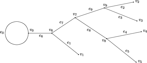As an example see Figure 1 where $r=9,p=5,\mathit{\sigma }=4.$

Let $d_j$ be the length of the edge $e_j$, $j=\overline{0,r}.$ Each edge $e\in \mathcal{E}$ is viewed as a segment $[0,d_j]$ and is parameterized by the parameter $x_j\in [0,d_j].$ It is convenient for us to choose the following orientation: for $j=\overline{1,r}$ the end vertex $v_j$ corresponds to $x_j=0$, and the initial vertex $v_{j_k}$ corresponds to $x_j=d_j$; for the cycle $e_0$ both endpoints $x_0=+0$ and $x_0=d_0-0$ correspond to $v_0$.

Figure 1. A graph with a rooted cycle.

A function Y on G may be represented as $Y={\{y_j\}}_{j=\overline{0,r}}$, where the function $y_j(x_j)$ is defined on the edge $e_j$. Let $q={\{q_j\}}_{j=\overline{0,r}}$ and $p={\{p_j\}}_{j=\overline{0,r}}$ be complex-valued functions on G; they are called the potentials. Assume that $q_j(x_j)\in L(0,d_j),$$p_j(x_j)\in AC[0,d_j].$ Consider the following differential equation on G:(1.1) $$\begin{array}{c}\hfill y_j^{″}(x_j)+({\mathit{\rho }}^2+\mathit{\rho }{p}_j(x)+q_j(x_j))y_j(x_j)=0,x_j\in [0,d_j],\end{array}$$(1.1)

where $j=\overline{0,r}$, $\mathit{\rho }$ is the spectral parameter, the functions $y_j(x_j),y_j^{\prime }(x_j)$ are absolutely continuous on $[0,d_j]$ and satisfy the following matching conditions in the internal vertices $v_0$ and $v_k$, $k=\overline{p+1,r}$: For $k=\overline{p+1,r}$,(1.2) $$\begin{array}{c}\hfill {\displaystyle y_j(d_j)=y_k(0)\text{for all}{e}_j\in R(v_k),\sum _{e_j\in R(v_k)}{y}_j^{\prime }(d_j)=y_k^{\prime }(0),}\end{array}$$(1.2)

and for $v_0$,(1.3) $$\begin{array}{c}\hfill y_{p+1}(d_{p+1})=y_0(d_0)=y_0(0),y_{p+1}^{\prime }(d_{p+1})+y_0^{\prime }(d_0)=y_0^{\prime }(0).\end{array}$$(1.3)

Matching conditions (1.2(1.2) $$\begin{array}{c}\hfill {\displaystyle y_j(d_j)=y_k(0)\text{for all}{e}_j\in R(v_k),\sum _{e_j\in R(v_k)}{y}_j^{\prime }(d_j)=y_k^{\prime }(0),}\end{array}$$(1.2) ) and (1.3(1.3) $$\begin{array}{c}\hfill y_{p+1}(d_{p+1})=y_0(d_0)=y_0(0),y_{p+1}^{\prime }(d_{p+1})+y_0^{\prime }(d_0)=y_0^{\prime }(0).\end{array}$$(1.3) ) are called the standard conditions. In electrical circuits, they express Kirchhoff’s law; in elastic string network, they express the balance of tension, and so on. Let us consider the boundary value problem $L_0(G)$ for Equation (1.1(1.1) $$\begin{array}{c}\hfill y_j^{″}(x_j)+({\mathit{\rho }}^2+\mathit{\rho }{p}_j(x)+q_j(x_j))y_j(x_j)=0,x_j\in [0,d_j],\end{array}$$(1.1) ) with the matching conditions (1.2(1.2) $$\begin{array}{c}\hfill {\displaystyle y_j(d_j)=y_k(0)\text{for all}{e}_j\in R(v_k),\sum _{e_j\in R(v_k)}{y}_j^{\prime }(d_j)=y_k^{\prime }(0),}\end{array}$$(1.2) ) and (1.3(1.3) $$\begin{array}{c}\hfill y_{p+1}(d_{p+1})=y_0(d_0)=y_0(0),y_{p+1}^{\prime }(d_{p+1})+y_0^{\prime }(d_0)=y_0^{\prime }(0).\end{array}$$(1.3) ) and with the Dirichlet boundary conditions at the boundary vertices $v_1,\dots ,v_p$:$$y_j(0)=0,j=\overline{1,p}.$$

Moreover, we also consider the boundary value problems $L_k(G)$, $k=\overline{1,p}$ for Equation (1.1(1.1) $$\begin{array}{c}\hfill y_j^{″}(x_j)+({\mathit{\rho }}^2+\mathit{\rho }{p}_j(x)+q_j(x_j))y_j(x_j)=0,x_j\in [0,d_j],\end{array}$$(1.1) ) with the matching conditions (1.2(1.2) $$\begin{array}{c}\hfill {\displaystyle y_j(d_j)=y_k(0)\text{for all}{e}_j\in R(v_k),\sum _{e_j\in R(v_k)}{y}_j^{\prime }(d_j)=y_k^{\prime }(0),}\end{array}$$(1.2) ) and (1.3(1.3) $$\begin{array}{c}\hfill y_{p+1}(d_{p+1})=y_0(d_0)=y_0(0),y_{p+1}^{\prime }(d_{p+1})+y_0^{\prime }(d_0)=y_0^{\prime }(0).\end{array}$$(1.3) ) and with the boundary conditions$$y_k^{\prime }(0)=0,y_j(0)=0,j=\overline{1,p}\backslash k.$$

We denote by ${\mathrm{\Lambda }}_k=\{{\mathit{\rho }}_{kn}\},$$k=\overline{0,p},$ the eigenvalues (counting with multiplicities) of $L_k(G)$. In contrast to the case of trees (see [14,30]), here the specification of the spectra ${\mathrm{\Lambda }}_k$, $k=\overline{0,p},$ does not uniquely determines the potentials, and we need an additional information. Let $S_j(x_j,\mathit{\rho }),C_j(x_j,\mathit{\rho }),j=\overline{0,r}$ be the solutions of equation (1.1) on the edge $e_j$ with the initial conditions $S_j(0,\mathit{\rho })=C_j^{\prime }(0,\mathit{\rho })=0,S_j^{\prime }(0,\mathit{\rho })=C_j(0,\mathit{\rho })=1.$ For each fixed $x_j\in [0,d_j],$ the functions $S_j^{(\mathit{\nu })}(x_j,\mathit{\rho }),C_j^{(\mathit{\nu })}(x_j,\mathit{\rho }),$$j=\overline{0,r},\mathit{\nu }=0,1,$ are entire in $\mathit{\rho }$ of exponential type. Moreover, $⟨C_j(x_j,\mathit{\rho }),S_j(x_j,\mathit{\rho })⟩\equiv 1,$ where $⟨y,z⟩:=y{z}^{\prime }-y^{\prime }z$ is the Wronskian of y and z. Denote$$a(\mathit{\rho }):=C_0(d_0,\mathit{\rho })-S_0^{\prime }(d_0,\mathit{\rho }),h(\mathit{\rho }):=S_0(d_0,\mathit{\rho }).$$

Let $\mathcal{V}=\{{\mathit{\nu }}_n\}$ be zeros (counting with multiplicities) of the entire function $h(\mathit{\rho }).$ Then $\{{\mathit{\nu }}_n\}$ are the eigenvalues of the boundary value problem $\mathcal{B}$ for Equation (1.1(1.1) $$\begin{array}{c}\hfill y_j^{″}(x_j)+({\mathit{\rho }}^2+\mathit{\rho }{p}_j(x)+q_j(x_j))y_j(x_j)=0,x_j\in [0,d_j],\end{array}$$(1.1) ) with $j=0$ under the boundary conditions $y_0(0)=y_0(d_0)=0.$ Let $\mathrm{\Omega }=\{{\mathit{\omega }}_n\}$ be the $\mathrm{\Omega }$-sequence for $\mathcal{B}$ (see [32]). For example, if all zeros of $h(\mathit{\rho })$ are simple, then$${\mathit{\omega }}_n=\left\{\begin{array}{cc}0,\hfill & a({\mathit{\nu }}_n)=0,\hfill \\ +1,\hfill & a({\mathit{\nu }}_n)\ne 0,\text{arg}a({\mathit{\nu }}_n)\in [0,\mathit{\pi }),\hfill \\ -1,\hfill & a({\mathit{\nu }}_n)\ne 0,\text{arg}a({\mathit{\nu }}_n)\in [\mathit{\pi },2\mathit{\pi }).\hfill \end{array}\right.$$

We note that for the classical self-adjoint periodic Sturm–Liouville inverse problem, the $\mathrm{\Omega }$-sequence was introduced and studied in [33,34] and other works. The inverse problem is formulated as follows.

Inverse Problem 1.1:

Given ${\mathrm{\Lambda }}_k,k=\overline{0,p}$ and $\mathrm{\Omega },$ construct q and p on G.

Let us formulate the uniqueness theorem for the solution of inverse problem 1.1. For this purpose together with (p, q) we consider potentials $(\tilde{p},\tilde{q}).$ Everywhere below if a symbol $\mathit{\mu }$ denotes an object related to (p, q) then $\tilde{\mathit{\mu }}$ will denote the analogous object related to $(\tilde{p},\tilde{q}).$

Theorem 1.2:

If ${\mathrm{\Lambda }}_k={\tilde{\mathrm{\Lambda }}}_k,k=\overline{0,p},$ and $\mathrm{\Omega }=\tilde{\mathrm{\Omega }},$ then $q=\tilde{q}$ and $p=\tilde{p}$ on G. Thus, the specification of ${\mathrm{\Lambda }}_k,k=\overline{0,p}$ and $\mathrm{\Omega }$ uniquely determines the potentials q and p on G.

This theorem will be proved in Section 3. Moreover, we will give there a constructive procedure for the solution of inverse problem 1.1. In Section 2 we introduce the main notions and prove some auxiliary propositions.

2. Characteristic functions

Fix $k=\overline{p+1,r}.$ Denote $Q_k:=\{z\in T:v_k<z\},G_k:=\overline{G\backslash Q_k}$. Then$$Q_k=\bigcup _{e_i\in R(v_k)}{T}_{ki},$$

where $T_{ki}$ is the tree with the root $v_k$ and with the rooted edge $e_i$. Clearly, $G_k=e_0\cup T_k$, where $T_k=\overline{T\backslash Q_k}$.

Noatations:

If D is a graph, then we will denote by $L_0(D)$ the boundary value problem for Equation (1.1(1.1) $$\begin{array}{c}\hfill y_j^{″}(x_j)+({\mathit{\rho }}^2+\mathit{\rho }{p}_j(x)+q_j(x_j))y_j(x_j)=0,x_j\in [0,d_j],\end{array}$$(1.1) ) on D with the standard matching conditions in internal vertices and with the Dirichlet boundary conditions in boundary vertices. Let ${\{Y\}}_D:={\{y_j\}}_{e_j\in D}.$ If $v_j$ is a boundary vertex of D,  then $L_j(D)$ will denote the boundary value problem for Equation (1.1(1.1) $$\begin{array}{c}\hfill y_j^{″}(x_j)+({\mathit{\rho }}^2+\mathit{\rho }{p}_j(x)+q_j(x_j))y_j(x_j)=0,x_j\in [0,d_j],\end{array}$$(1.1) ) on D with the standard matching conditions in internal vertices, with the Neumann boundary condition $Y_{|v_j}^{\prime }=0$ at $v_j$ and with the Dirichlet boundary conditions in all other boundary vertices. For example, $L_0(G_k)$ is the boundary value problem on $G_k$ with the boundary conditions $y_m(0)=0,$$e_m\in E\cap G_k$, and $L_k(G_k)$ is the boundary value problem on $G_k$ with the boundary conditions $y_k^{\prime }(0)=0,$$y_m(0)=0,$$e_m\in (E\cap G_k)\backslash e_k$. We also consider the BVP $L^1(T)$ for Equation (1.1(1.1) $$\begin{array}{c}\hfill y_j^{″}(x_j)+({\mathit{\rho }}^2+\mathit{\rho }{p}_j(x)+q_j(x_j))y_j(x_j)=0,x_j\in [0,d_j],\end{array}$$(1.1) ) on T with the boundary conditions $Y_{|v_0}^{\prime }=0,Y_{|v_j}=0,j=\overline{1,p}.$

Fix $k=\overline{1,p}.$ Let ${\mathrm{\Phi }}_k={\{{\mathrm{\Phi }}_{kj}\}}_{j=\overline{0,r}}$, be solutions of Equation (1.1(1.1) $$\begin{array}{c}\hfill y_j^{″}(x_j)+({\mathit{\rho }}^2+\mathit{\rho }{p}_j(x)+q_j(x_j))y_j(x_j)=0,x_j\in [0,d_j],\end{array}$$(1.1) ) satisfying the matching conditions (1.2(1.2) $$\begin{array}{c}\hfill {\displaystyle y_j(d_j)=y_k(0)\text{for all}{e}_j\in R(v_k),\sum _{e_j\in R(v_k)}{y}_j^{\prime }(d_j)=y_k^{\prime }(0),}\end{array}$$(1.2) ) and (1.3(1.3) $$\begin{array}{c}\hfill y_{p+1}(d_{p+1})=y_0(d_0)=y_0(0),y_{p+1}^{\prime }(d_{p+1})+y_0^{\prime }(d_0)=y_0^{\prime }(0).\end{array}$$(1.3) ) and the boundary conditions(2.1) $$\begin{array}{c}\hfill {\mathrm{\Phi }}_{kj}(0,\mathit{\rho })={\mathit{\delta }}_{kj},j=\overline{1,p},\end{array}$$(2.1)

where ${\mathit{\delta }}_{kj}$ is the Kronecker symbol. Denote $M_k(\mathit{\rho }):={\mathrm{\Phi }}_{kk}^{\prime }(0,\mathit{\rho }),$$k=\overline{1,p}.$ The function $M_k(\mathit{\rho },G):=M_k(\mathit{\rho })$ is called the Weyl function with respect to the boundary vertex $v_k$.

Denote $M_{kj}^0(\mathit{\rho })={\mathrm{\Phi }}_{kj}^{\prime }(0,\mathit{\rho })$, $M_{kj}^1(\mathit{\rho })={\mathrm{\Phi }}_{kj}(0,\mathit{\rho }),$$j=\overline{0,r}$. Then(2.2) $$\begin{array}{c}\hfill {\mathrm{\Phi }}_{kj}(x_j,\mathit{\rho })=M_{kj}^1(\mathit{\rho })C_j(x_j,\mathit{\rho })+M_{kj}^0(\mathit{\rho })S_j(x_j,\mathit{\rho }),j=\overline{0,r}.\end{array}$$(2.2)

In particular, $M_{kk}^0(\mathit{\rho })=M_k(\mathit{\rho },G)$, $M_{kk}^1(\mathit{\rho })=1$, $M_{kj}^1(\mathit{\rho })=0$ for $j=\overline{1,p}\backslash k$. Hence$${\mathrm{\Phi }}_{kk}(x_k,\mathit{\rho })=C_k(x_k,\mathit{\rho })+M_k(\mathit{\rho },G)S_k(x_k,\mathit{\rho }),$$

and consequently, $⟨{\mathrm{\Phi }}_{kk}(x_k,\mathit{\rho }),S_k(x_k,\mathit{\rho })⟩\equiv 1.$ Substituting (2.2(2.2) $$\begin{array}{c}\hfill {\mathrm{\Phi }}_{kj}(x_j,\mathit{\rho })=M_{kj}^1(\mathit{\rho })C_j(x_j,\mathit{\rho })+M_{kj}^0(\mathit{\rho })S_j(x_j,\mathit{\rho }),j=\overline{0,r}.\end{array}$$(2.2) ) into (1.2(1.2) $$\begin{array}{c}\hfill {\displaystyle y_j(d_j)=y_k(0)\text{for all}{e}_j\in R(v_k),\sum _{e_j\in R(v_k)}{y}_j^{\prime }(d_j)=y_k^{\prime }(0),}\end{array}$$(1.2) ), (1.3(1.3) $$\begin{array}{c}\hfill y_{p+1}(d_{p+1})=y_0(d_0)=y_0(0),y_{p+1}^{\prime }(d_{p+1})+y_0^{\prime }(d_0)=y_0^{\prime }(0).\end{array}$$(1.3) ) and (2.1(2.1) $$\begin{array}{c}\hfill {\mathrm{\Phi }}_{kj}(0,\mathit{\rho })={\mathit{\delta }}_{kj},j=\overline{1,p},\end{array}$$(2.1) ) we obtain a linear algebraic system $s_k$ with respect to $M_{kj}^0(\mathit{\rho }),M_{kj}^1(\mathit{\rho }),$$j=\overline{0,r}.$ The determinant ${\mathrm{\Delta }}_0(\mathit{\rho },G)$ of this system does not depend on k and has the form(2.3) $$\begin{array}{c}\hfill {\mathrm{\Delta }}_0(\mathit{\rho },G)={\mathrm{\Delta }}_0(\mathit{\rho },T)d(\mathit{\rho })+{\mathrm{\Delta }}^1(\mathit{\rho },T)h(\mathit{\rho }),\end{array}$$(2.3)

where(2.4) $$\begin{array}{c}\hfill d(\mathit{\rho })=C_0(d_0,\mathit{\rho })+S_0^{\prime }(d_0,\mathit{\rho })-2,h(\mathit{\rho })=S_0(d_0,\mathit{\rho }),\end{array}$$(2.4) ${\mathrm{\Delta }}_0(\mathit{\rho },T)$ and ${\mathrm{\Delta }}^1(\mathit{\rho },T)$ are the characteristic functions of the boundary value problems $L_0(T)$ and $L^1(T)$ respectively, which were defined and studied in [35]. For convenience of the readers in the Appendix 1 at the end of the paper we provide formulae for constructing the functions ${\mathrm{\Delta }}_0(\mathit{\rho },T)$ and ${\mathrm{\Delta }}^1(\mathit{\rho },T)$ from [35]. The function ${\mathrm{\Delta }}_0(\mathit{\rho },G)$ is entire in $\mathit{\rho }$ of exponential type, and its zeros (counting with multiplicities) coincide with the eigenvalues of the boundary value problem $L_0(G).$ This fact and other similar facts can be shown by the well-known arguments (see, e.g. [11,14,35,37]). Solving the algebraic system $s_k$ we get by Cramer’s rule: $M_{kj}^{\mathit{\nu }}(\mathit{\rho })={\mathrm{\Delta }}_{kj}^{\mathit{\nu }}(\mathit{\rho },G)/{\mathrm{\Delta }}_0(\mathit{\rho },G)$, $\mathit{\nu }=0,1,j=\overline{0,r},$ where the determinant ${\mathrm{\Delta }}_{kj}^{\mathit{\nu }}(\mathit{\rho },G)$ is obtained from ${\mathrm{\Delta }}_0(\mathit{\rho },G)$ by the replacement of the column which corresponds to $M_{kj}^{\mathit{\nu }}(\mathit{\rho })$ with the column of free terms. In particular,(2.5) $$\begin{array}{c}\hfill {\displaystyle M_k(\mathit{\rho },G)=-\frac{{\mathrm{\Delta }}_k(\mathit{\rho },G)}{{\mathrm{\Delta }}_0(\mathit{\rho },G)},k=\overline{1,p},}\end{array}$$(2.5)

where ${\mathrm{\Delta }}_k(\mathit{\rho },G),k=\overline{1,p},$ is obtained from ${\mathrm{\Delta }}_0(\mathit{\rho },G)$ by the replacement of $S_k^{(\mathit{\nu })}(d_k,\mathit{\rho }),$$\mathit{\nu }=0,1,$ with $C_k^{(\mathit{\nu })}(d_k,\mathit{\rho }).$ Similarly to the function ${\mathrm{\Delta }}_0(\mathit{\rho },G),$ one can see that the zeros of ${\mathrm{\Delta }}_k(\mathit{\rho },G)$ (counting with multiplicities) coincide with the eigenvalues of the boundary value problem $L_k(G).$ The function ${\mathrm{\Delta }}_k(\mathit{\rho },G),k=\overline{0,p},$ is called the characteristic function for the boundary value problem $L_k(G).$

Fix $k=\overline{p+1,r}.$ Let ${\mathrm{\Delta }}_0(\mathit{\rho },G_k)$ and ${\mathrm{\Delta }}_k(\mathit{\rho },G_k)$ be the characteristic functions for $L_0(G_k)$ and $L_k(G_k)$, respectively. Using (2.3(2.3) $$\begin{array}{c}\hfill {\mathrm{\Delta }}_0(\mathit{\rho },G)={\mathrm{\Delta }}_0(\mathit{\rho },T)d(\mathit{\rho })+{\mathrm{\Delta }}^1(\mathit{\rho },T)h(\mathit{\rho }),\end{array}$$(2.3) ) and (2.4(2.4) $$\begin{array}{c}\hfill d(\mathit{\rho })=C_0(d_0,\mathit{\rho })+S_0^{\prime }(d_0,\mathit{\rho })-2,h(\mathit{\rho })=S_0(d_0,\mathit{\rho }),\end{array}$$(2.4) ) and formulae for ${\mathrm{\Delta }}_0(\mathit{\rho },T),$${\mathrm{\Delta }}^1(\mathit{\rho },T)$ from [35] (see also the Appendix 1) one can get(2.6) $$\begin{array}{c}\hfill {\mathrm{\Delta }}_0(\mathit{\rho },G)={\mathrm{\Delta }}_0(\mathit{\rho },Q_k){\mathrm{\Delta }}_0(\mathit{\rho },G_k)+\left(\prod _{e_i\in R(v_k)}{\mathrm{\Delta }}_0(\mathit{\rho },T_{ki})\right){\mathrm{\Delta }}_k(\mathit{\rho },G_k),\end{array}$$(2.6)

where ${\mathrm{\Delta }}_0(\mathit{\rho },Q_k)$ and ${\mathrm{\Delta }}_0(\mathit{\rho },T_{ki})$ are the characteristic functions for $L_0(Q_k)$ and $L_0(T_{ki})$, respectively, which were defined and studied in [35] (see also the Appendix 1). Similarly, for $e_j\in E\cap T_{ks}$,(2.7) $$\begin{array}{c}\hfill {\mathrm{\Delta }}_j(\mathit{\rho },G)={\mathrm{\Delta }}_j(\mathit{\rho },Q_k){\mathrm{\Delta }}_0(\mathit{\rho },G_k)+\left({\mathrm{\Delta }}_j(\mathit{\rho },T_{ks})\prod _{e_i\in R(v_k),i\ne s}{\mathrm{\Delta }}_0(\mathit{\rho },T_{ki})\right){\mathrm{\Delta }}_k(\mathit{\rho },G_k),\end{array}$$(2.7)

where ${\mathrm{\Delta }}_j(\mathit{\rho },Q_k)$ and ${\mathrm{\Delta }}_j(\mathit{\rho },T_{ki})$ are constructed from ${\mathrm{\Delta }}_0(\mathit{\rho },Q_k)$ and ${\mathrm{\Delta }}_0(\mathit{\rho },T_{ki})$ by the replacement of $S_j^{(\mathit{\nu })}(d_j,\mathit{\rho }),$$\mathit{\nu }=0,1,$ with $C_j^{(\mathit{\nu })}(d_j,\mathit{\rho }).$

Example 2.1:

Let $\mathit{\sigma }=1.$ Then $r=1,$$${\mathrm{\Delta }}_0(\mathit{\rho },G)=S_1(d_1,\mathit{\rho })d(\mathit{\rho })+S_1^{\prime }(d_1,\mathit{\rho })h(\mathit{\rho }),{\mathrm{\Delta }}_0(\mathit{\rho },T)=S_1(d_1,\mathit{\rho }),{\mathrm{\Delta }}^1(\mathit{\rho },T)=S_1^{\prime }(d_1,\mathit{\rho }).$$

Example 2.2:

Let $\mathit{\sigma }=2.$ Then $r=p+1,$$T_{p+1,i}=\{e_i\},$$i=\overline{1,p},$ hence$$\begin{array}{cc}\hfill {\mathrm{\Delta }}_0(\mathit{\rho },T)& =\prod _{m=1}^p{S}_m(d_m,\mathit{\rho })\left(\sum _{i=1}^p\frac{S_i^{\prime }(d_i,\mathit{\rho })}{S_i(d_i,\mathit{\rho })}{S}_{p+1}(d_{p+1},\mathit{\rho })+C_{p+1}(d_{p+1},\mathit{\rho })\right),\hfill \\ \hfill {\mathrm{\Delta }}^1(\mathit{\rho },T)& =\prod _{m=1}^p{S}_m(d_m,\mathit{\rho })\left(\sum _{i=1}^p\frac{S_i^{\prime }(d_i,\mathit{\rho })}{S_i(d_i,\mathit{\rho })}{S}_{p+1}^{\prime }(d_{p+1},\mathit{\rho })+C_{p+1}^{\prime }(d_{p+1},\mathit{\rho })\right).\hfill \end{array}$$

In particular, for $p=2,$$$\begin{array}{cc}\hfill {\mathrm{\Delta }}_0(\mathit{\rho },T)& =(S_1(d_1,\mathit{\rho })S_2^{\prime }(d_2,\mathit{\rho })+S_1^{\prime }(d_1,\mathit{\rho })S_2(d_2,\mathit{\rho }))S_3(d_3,\mathit{\rho })+S_1(d_1,\mathit{\rho })S_2(d_2,\mathit{\rho })C_3(d_3,\mathit{\rho }),\hfill \\ \hfill {\mathrm{\Delta }}^1(\mathit{\rho },T)& =(S_1(d_1,\mathit{\rho })S_2^{\prime }(d_2,\mathit{\rho })+S_1^{\prime }(d_1,\mathit{\rho })S_2(d_2,\mathit{\rho }))S_3^{\prime }(d_3,\mathit{\rho })+S_1(d_1,\mathit{\rho })S_2(d_2,\mathit{\rho })C_3^{\prime }(d_3,\mathit{\rho }),\hfill \end{array}$$

and (2.6(2.6) $$\begin{array}{c}\hfill {\mathrm{\Delta }}_0(\mathit{\rho },G)={\mathrm{\Delta }}_0(\mathit{\rho },Q_k){\mathrm{\Delta }}_0(\mathit{\rho },G_k)+\left(\prod _{e_i\in R(v_k)}{\mathrm{\Delta }}_0(\mathit{\rho },T_{ki})\right){\mathrm{\Delta }}_k(\mathit{\rho },G_k),\end{array}$$(2.6) ) takes the form$$\begin{array}{cc}\hfill {\mathrm{\Delta }}_0(\mathit{\rho },G)& =(S_1(d_1,\mathit{\rho })S_2^{\prime }(d_2,\mathit{\rho })+S_1^{\prime }(d_1,\mathit{\rho })S_2(d_2,\mathit{\rho }))(S_3(d_3,\mathit{\rho })d(\mathit{\rho })+S_3^{\prime }(d_3,\mathit{\rho })h(\mathit{\rho }))\hfill \\ \hfill & +S_1(d_1,\mathit{\rho })S_2(d_2,\mathit{\rho })(C_3(d_3,\mathit{\rho })d(\mathit{\rho })+C_3^{\prime }(d_3,\mathit{\rho })h(\mathit{\rho }))\hfill \\ \hfill & ={\mathrm{\Delta }}_0(\mathit{\rho },Q_3){\mathrm{\Delta }}_0(\mathit{\rho },G_3)+{\mathrm{\Delta }}_0(\mathit{\rho },T_{31}){\mathrm{\Delta }}_0(\mathit{\rho },T_{32}){\mathrm{\Delta }}_3(\mathit{\rho },G_3),\hfill \end{array}$$

where$$\begin{array}{cc}\hfill {\mathrm{\Delta }}_0(\mathit{\rho },Q_3)& =S_1(d_1,\mathit{\rho })S_2^{\prime }(d_2,\mathit{\rho })+S_1^{\prime }(d_1,\mathit{\rho })S_2(d_2,\mathit{\rho }),{\mathrm{\Delta }}_0(\mathit{\rho },G_3)=S_3(d_3,\mathit{\rho })d(\mathit{\rho })+S_3^{\prime }(d_3,\mathit{\rho })h(\mathit{\rho }),\hfill \\ \hfill {\mathrm{\Delta }}_0(\mathit{\rho },T_{31})& =S_1(d_1,\mathit{\rho }),{\mathrm{\Delta }}_0(\mathit{\rho },T_{32})=S_2(d_2,\mathit{\rho }),{\mathrm{\Delta }}_3(\mathit{\rho },G_3)=C_3(d_3,\mathit{\rho })d(\mathit{\rho })+C_3^{\prime }(d_3,\mathit{\rho })h(\mathit{\rho }).\hfill \end{array}$$

Denote$$\begin{array}{cc}\hfill {\mathcal{E}}_k(x_k)& =\frac{1}{2}{\int }_0^{x_k}{p}_k(t)\mathrm{d}t,{\mathit{\theta }}_k=\frac{1}{2d_k}{\int }_0^{d_k}{p}_k(t)\mathrm{d}t,E^{\pm }(\mathit{\rho })=\prod _{j=0}^{r}exp(\mp i(\mathit{\rho }+{\mathit{\theta }}_j)d_j),\hfill \\ \hfill d& :=\sum _{j=0}^r{\mathit{\theta }}_j{d}_j=\frac{1}{2}\sum _{j=0}^r{\int }_0^{d_j}{p}_j(t)\mathrm{d}t,\mathit{\tau }=\text{Im}\mathit{\rho },\hfill \\ \hfill {\mathrm{\Pi }}^{\pm }& =\{\mathit{\rho }:\pm \mathit{\tau }\ge 0\},{\mathrm{\Pi }}_{\mathit{\delta }}^{+}=\{\mathit{\rho }:arg\mathit{\rho }\in [\mathit{\delta },\mathit{\pi }-\mathit{\delta }]\},{\mathrm{\Pi }}_{\mathit{\delta }}^{-}=\{\mathit{\rho }:arg\mathit{\rho }\in [\mathit{\pi }+\mathit{\delta },2\mathit{\pi }-\mathit{\delta }]\}.\hfill \end{array}$$

Without loss of generality we assume that $d=0.$ It is known (see [36]) that for each fixed $j=\overline{0,r}$ on the edge $e_j,$ there exist fundamental systems of solutions of Equation (1.1(1.1) $$\begin{array}{c}\hfill y_j^{″}(x_j)+({\mathit{\rho }}^2+\mathit{\rho }{p}_j(x)+q_j(x_j))y_j(x_j)=0,x_j\in [0,d_j],\end{array}$$(1.1) ) $\{e_{j1}^{\pm }(x_j,\mathit{\rho }),e_{j2}^{\pm }(x_j,\mathit{\rho })\}$, $x_j\in [0,d_j],\mathit{\rho }\in {\mathrm{\Pi }}^{\pm },|\mathit{\rho }|\ge {\mathit{\rho }}^{\ast }$ with the properties:

(1)

the functions $\frac{d^{\mathit{\nu }}}{d{x}_j^{\mathit{\nu }}}{e}_{js}^{\pm }(x_j,\mathit{\rho }),\mathit{\nu }=0,1,$ are continuous for $x_j\in [0,d_j],\mathit{\rho }\in {\mathrm{\Pi }}^{\pm },|\mathit{\rho }|\ge {\mathit{\rho }}^{\ast }$, and are analytic with respect to $\mathit{\rho }$ for $\pm \text{Im}\mathit{\rho }>0,|\mathit{\rho }|>{\mathit{\rho }}^{\ast }$;

(2)

uniformly for $x_j\in [0,d_j],$ the following asymptotical formulae hold(2.8) $$\begin{array}{cc}\hfill \frac{{\mathrm{d}}^{\mathit{\nu }}}{\mathrm{d}{x}_j^{\mathit{\nu }}}{e}_{j1}^{\pm }(x_j,\mathit{\rho })& ={(i\mathit{\rho })}^{\mathit{\nu }}exp(i(\mathit{\rho }{x}_j+{\mathcal{E}}_j(x_j)))[1],\hfill \\ \hfill \frac{{\mathrm{d}}^{\mathit{\nu }}}{\mathrm{d}{x}_j^{\mathit{\nu }}}{e}_{j2}^{\pm }(x_j,\mathit{\rho })& ={(-i\mathit{\rho })}^{\mathit{\nu }}exp(-i(\mathit{\rho }{x}_j+{\mathcal{E}}_j(x_j)))[1],\hfill \end{array}$$(2.8) where $\mathit{\rho }\in {\mathrm{\Pi }}^{\pm },|\mathit{\rho }|\to \infty ,[1]=1+O({\mathit{\rho }}^{-1}),\mathit{\nu }=0,1.$

Fix $k=\overline{1,p}.$ One has(2.9) $$\begin{array}{c}\hfill {\mathrm{\Phi }}_{kj}(x_j,\mathit{\rho })=A_{kj}^{\pm }(\mathit{\rho })e_{j1}^{\pm }(x_j,\mathit{\rho })+B_{kj}^{\pm }(\mathit{\rho })e_{j2}^{\pm }(x_j,\mathit{\rho }),\mathit{\rho }\in {\mathrm{\Pi }}^{\pm },x_j\in [0,d_j],j=\overline{0,r}.\end{array}$$(2.9)

Substituting (2.9(2.9) $$\begin{array}{c}\hfill {\mathrm{\Phi }}_{kj}(x_j,\mathit{\rho })=A_{kj}^{\pm }(\mathit{\rho })e_{j1}^{\pm }(x_j,\mathit{\rho })+B_{kj}^{\pm }(\mathit{\rho })e_{j2}^{\pm }(x_j,\mathit{\rho }),\mathit{\rho }\in {\mathrm{\Pi }}^{\pm },x_j\in [0,d_j],j=\overline{0,r}.\end{array}$$(2.9) ) into (1.2(1.2) $$\begin{array}{c}\hfill {\displaystyle y_j(d_j)=y_k(0)\text{for all}{e}_j\in R(v_k),\sum _{e_j\in R(v_k)}{y}_j^{\prime }(d_j)=y_k^{\prime }(0),}\end{array}$$(1.2) ), (1.3(1.3) $$\begin{array}{c}\hfill y_{p+1}(d_{p+1})=y_0(d_0)=y_0(0),y_{p+1}^{\prime }(d_{p+1})+y_0^{\prime }(d_0)=y_0^{\prime }(0).\end{array}$$(1.3) ) and (2.1(2.1) $$\begin{array}{c}\hfill {\mathrm{\Phi }}_{kj}(0,\mathit{\rho })={\mathit{\delta }}_{kj},j=\overline{1,p},\end{array}$$(2.1) ) we obtain a linear algebraic system $s_k^{\pm }$ with respect to $A_{kj}^{\pm }(\mathit{\rho }),B_{kj}^{\pm }(\mathit{\rho }),$$j=\overline{0,r}.$ The determinant ${\mathit{\delta }}^{\pm }(\mathit{\rho })$ of $s_k^{\pm }$ does not depend on k,  and has the form(2.10) $$\begin{array}{c}\hfill {\mathit{\delta }}^{\pm }(\mathit{\rho })=({\mathit{\delta }}_0^{\pm }+O(\frac{1}{\mathit{\rho }})){\mathit{\rho }}^{r+1-p}{E}^{\pm }(\mathit{\rho }),{\mathit{\delta }}_0^{\pm }\ne 0,\mathit{\rho }\in {\mathrm{\Pi }}_{\mathit{\delta }}^{\pm },|\mathit{\rho }|\to \infty .\end{array}$$(2.10)

Solving the algebraic system $s_k^{\pm }$ and using (2.8(2.8) $$\begin{array}{cc}\hfill \frac{{\mathrm{d}}^{\mathit{\nu }}}{\mathrm{d}{x}_j^{\mathit{\nu }}}{e}_{j1}^{\pm }(x_j,\mathit{\rho })& ={(i\mathit{\rho })}^{\mathit{\nu }}exp(i(\mathit{\rho }{x}_j+{\mathcal{E}}_j(x_j)))[1],\hfill \\ \hfill \frac{{\mathrm{d}}^{\mathit{\nu }}}{\mathrm{d}{x}_j^{\mathit{\nu }}}{e}_{j2}^{\pm }(x_j,\mathit{\rho })& ={(-i\mathit{\rho })}^{\mathit{\nu }}exp(-i(\mathit{\rho }{x}_j+{\mathcal{E}}_j(x_j)))[1],\hfill \end{array}$$(2.8) )–(2.10(2.10) $$\begin{array}{c}\hfill {\mathit{\delta }}^{\pm }(\mathit{\rho })=({\mathit{\delta }}_0^{\pm }+O(\frac{1}{\mathit{\rho }})){\mathit{\rho }}^{r+1-p}{E}^{\pm }(\mathit{\rho }),{\mathit{\delta }}_0^{\pm }\ne 0,\mathit{\rho }\in {\mathrm{\Pi }}_{\mathit{\delta }}^{\pm },|\mathit{\rho }|\to \infty .\end{array}$$(2.10) ) we get for each fixed $x_k\in [0,d_k)$:(2.11) $$\begin{array}{c}\hfill {\mathrm{\Phi }}_{kk}^{(\mathit{\nu })}(x_k,\mathit{\rho })={(\pm i\mathit{\rho })}^{\mathit{\nu }}exp(\pm i(\mathit{\rho }{x}_k+{\mathcal{E}}_k(x_k)))[1],\mathit{\rho }\in {\mathrm{\Pi }}_{\mathit{\delta }}^{\pm },|\mathit{\rho }|\to \infty .\end{array}$$(2.11)

In particular,(2.12) $$\begin{array}{c}\hfill M_k(\mathit{\rho })=(\pm i\mathit{\rho })[1],\mathit{\rho }\in {\mathrm{\Pi }}_{\mathit{\delta }}^{\pm },|\mathit{\rho }|\to \infty .\end{array}$$(2.12)

Moreover, for $|\mathit{\rho }|\to \infty ,$$k=\overline{0,r},$ uniformly in $x_k\in [0,d_k],$(2.13) $$\begin{array}{c}\hfill {\displaystyle S_k^{(\mathit{\nu })}(x_k,\mathit{\rho })=\frac{1}{2{(-i\mathit{\rho })}^{1-\mathit{\nu }}}exp(-i(\mathit{\rho }{x}_k+{\mathcal{E}}_k(x_k)))[1]+\frac{1}{2{(i\mathit{\rho })}^{1-\mathit{\nu }}}exp(i(\mathit{\rho }{x}_k+{\mathcal{E}}_k(x_k)))[1].}\end{array}$$(2.13)

Similarly, one gets for $\mathit{\rho }\in {\mathrm{\Pi }}_{\mathit{\delta }}^{\pm },|\mathit{\rho }|\to \infty$:(2.14) $$\begin{array}{c}\hfill {\mathrm{\Delta }}_0(\mathit{\rho },G)=\frac{{\mathrm{\Delta }}_0^{\pm }}{{\mathit{\rho }}^p}{E}^{\pm }(\mathit{\rho })[1],{\mathrm{\Delta }}_0^{\pm }={(-2i)}^{-r-1}{\mathit{\delta }}_0^{\pm },\end{array}$$(2.14) (2.15) $$\begin{array}{c}\hfill {\mathrm{\Delta }}_k(\mathit{\rho },G)=\frac{(\mp i\mathit{\rho }){\mathrm{\Delta }}_0^{\pm }}{{\mathit{\rho }}^p}{E}^{\pm }(\mathit{\rho })[1],k=\overline{1,p}.\end{array}$$(2.15)

3. Solution of inverse problem 1.1

In this section, we provide a constructive procedure for the solution of inverse problem 1.1 and prove its uniqueness. First we consider the following auxiliary inverse problem for G on the edge $e_k$, $k=\overline{1,p},$ which is called IP(k).

IP(k). Given $M_k(\mathit{\rho },G),$construct $q_k(x_k),p_k(x_k),x_k\in [0,d_k].$

In IP(k) we construct the potentials only on the edge $e_k$, but the Weyl function $M_k(\mathit{\rho },G)$ brings a global information from the whole graph, i.e. IP(k) is not a local inverse problem related only to the edge $e_k$.

Lemma 3.1:

Fix $k=\overline{1,p}.$ The specification of two spectra ${\mathrm{\Lambda }}_0$ and ${\mathrm{\Lambda }}_k$ uniquely determines the Weyl function $M_k(\mathit{\rho },G).$

Proof:

The characteristic functions ${\mathrm{\Delta }}_k(\mathit{\rho },G),k=\overline{0,p},$ are entire in $\mathit{\rho }$ of exponential type. By Hadamard’s factorization theorem,(3.1) $$\begin{array}{c}\hfill {\mathrm{\Delta }}_k(\mathit{\rho },G)=B_{k}exp(A_k\mathit{\rho }){\mathrm{\Delta }}_k^{\ast }(\mathit{\rho },G),k=\overline{0,p},\end{array}$$(3.1)

where(3.2) $$\begin{array}{c}\hfill {\mathrm{\Delta }}_k^{\ast }(\mathit{\rho },G)={\mathit{\rho }}^{{\mathit{\xi }}_k}\prod _{n\in {\mathrm{\Lambda }}_k^{\prime }}(1-\frac{\mathit{\rho }}{{\mathit{\rho }}_{nk}})exp(\mathit{\rho }/{\mathit{\rho }}_{nk}),k=\overline{0,p},\end{array}$$(3.2) ${\mathrm{\Lambda }}_k^{\prime }=\{n:{\mathit{\rho }}_{nk}\ne 0\},$ and ${\mathit{\xi }}_k\ge 0$ is the multiplicity of the zero eigenvalue. In view of (2.5(2.5) $$\begin{array}{c}\hfill {\displaystyle M_k(\mathit{\rho },G)=-\frac{{\mathrm{\Delta }}_k(\mathit{\rho },G)}{{\mathrm{\Delta }}_0(\mathit{\rho },G)},k=\overline{1,p},}\end{array}$$(2.5) ) and (3.1(3.1) $$\begin{array}{c}\hfill {\mathrm{\Delta }}_k(\mathit{\rho },G)=B_{k}exp(A_k\mathit{\rho }){\mathrm{\Delta }}_k^{\ast }(\mathit{\rho },G),k=\overline{0,p},\end{array}$$(3.1) ), we deduce(3.3) $$\begin{array}{c}\hfill M_k(\mathit{\rho },G)=-b_{k}exp(a_k\mathit{\rho })\frac{{\mathrm{\Delta }}_k^{\ast }(\mathit{\rho },G)}{{\mathrm{\Delta }}_0^{\ast }(\mathit{\rho },G)},k=\overline{1,p},\end{array}$$(3.3)

where $b_k=B_k/B_0$, $a_k=A_k-A_0$. Using (2.12(2.12) $$\begin{array}{c}\hfill M_k(\mathit{\rho })=(\pm i\mathit{\rho })[1],\mathit{\rho }\in {\mathrm{\Pi }}_{\mathit{\delta }}^{\pm },|\mathit{\rho }|\to \infty .\end{array}$$(2.12) ) we calculate for $\mathit{\rho }\in {\mathrm{\Pi }}_{\mathit{\delta }}^{\pm },$$|\mathit{\rho }|\to \infty$:$$b_{k}exp(a_k\mathit{\rho })=\frac{(\mp i\mathit{\rho }){\mathrm{\Delta }}_0^{\ast }(\mathit{\rho },G)[1]}{{\mathrm{\Delta }}_k^{\ast }(\mathit{\rho },G)},$$

and consequently,(3.4) $$\begin{array}{cc}\hfill a_k& =\underset{|\mathit{\rho }|\to \infty }{lim}\frac{1}{\mathit{\rho }}ln(\frac{{\mathrm{\Delta }}_0^{\ast }(\mathit{\rho },G)}{{\mathrm{\Delta }}_k^{\ast }(\mathit{\rho },G)}),\mathit{\rho }\in {\mathrm{\Pi }}_{\mathit{\delta }}^{\pm },k=\overline{1,p},\hfill \end{array}$$(3.4) (3.5) $$\begin{array}{cc}\hfill b_k& =\underset{|\mathit{\rho }|\to \infty }{lim}\frac{(\mp i\mathit{\rho }){\mathrm{\Delta }}_0^{\ast }(\mathit{\rho },G)exp(-a_k\mathit{\rho })}{{\mathrm{\Delta }}_k^{\ast }(\mathit{\rho },G)},\mathit{\rho }\in {\mathrm{\Pi }}_{\mathit{\delta }}^{\pm },k=\overline{1,p}.\hfill \end{array}$$(3.5)

Thus, we have uniquely constructed $M_k(\mathit{\rho },G)$ by (3.2(3.2) $$\begin{array}{c}\hfill {\mathrm{\Delta }}_k^{\ast }(\mathit{\rho },G)={\mathit{\rho }}^{{\mathit{\xi }}_k}\prod _{n\in {\mathrm{\Lambda }}_k^{\prime }}(1-\frac{\mathit{\rho }}{{\mathit{\rho }}_{nk}})exp(\mathit{\rho }/{\mathit{\rho }}_{nk}),k=\overline{0,p},\end{array}$$(3.2) )–(3.5(3.5) $$\begin{array}{cc}\hfill b_k& =\underset{|\mathit{\rho }|\to \infty }{lim}\frac{(\mp i\mathit{\rho }){\mathrm{\Delta }}_0^{\ast }(\mathit{\rho },G)exp(-a_k\mathit{\rho })}{{\mathrm{\Delta }}_k^{\ast }(\mathit{\rho },G)},\mathit{\rho }\in {\mathrm{\Pi }}_{\mathit{\delta }}^{\pm },k=\overline{1,p}.\hfill \end{array}$$(3.5) ).$\square$

Let us prove the uniqueness theorem for the solution of IP(k).

Theorem 3.2:

If $M_k(\mathit{\rho },G)={\tilde{M}}_k(\mathit{\rho },G),$ then $p_k(x_k)={\tilde{p}}_k(x_k)$ and $q_k(x_k)={\tilde{q}}_k(x_k)$ a.e. on $[0,d_k].$ Thus, the specification of the Weyl function $M_k$ uniquely determines the potentials $p_k$ and $q_k$ on the edge $e_k$.

Proof:

Let us introduce the functions(3.6) $$\begin{array}{c}\hfill P_{1s}^k(x_k,\mathit{\rho })={(-1)}^s({\mathrm{\Phi }}_{kk}(x_k,\mathit{\rho }){\tilde{S}}_k^{(2-s)}(x_k,\mathit{\rho })-{\tilde{\mathrm{\Phi }}}_{kk}^{(2-s)}(x_k,\mathit{\rho })S_k(x_k,\mathit{\rho })),s=1,2.\end{array}$$(3.6)

Since $⟨{\mathrm{\Phi }}_{kk}(x_k,\mathit{\rho }),S_k(x_k,\mathit{\rho })⟩\equiv 1,$ it follows that(3.7) $$\begin{array}{c}\hfill S_k(x_k,\mathit{\rho })=P_{11}^k(x_k,\mathit{\rho }){\tilde{S}}_k(x_k,\mathit{\rho })+P_{12}^k(x_k,\mathit{\rho }){\tilde{S}}_k^{\prime }(x_k,\mathit{\rho }).\end{array}$$(3.7)

Denote ${\mathrm{\Omega }}_k(x_k)=cos{\widehat{\mathcal{E}}}_k(x_k),$ where ${\widehat{\mathcal{E}}}_k(x_k)={\mathcal{E}}_k(x_k)-{\tilde{\mathcal{E}}}_k(x_k).$ Taking (2.11(2.11) $$\begin{array}{c}\hfill {\mathrm{\Phi }}_{kk}^{(\mathit{\nu })}(x_k,\mathit{\rho })={(\pm i\mathit{\rho })}^{\mathit{\nu }}exp(\pm i(\mathit{\rho }{x}_k+{\mathcal{E}}_k(x_k)))[1],\mathit{\rho }\in {\mathrm{\Pi }}_{\mathit{\delta }}^{\pm },|\mathit{\rho }|\to \infty .\end{array}$$(2.11) ), (2.13(2.13) $$\begin{array}{c}\hfill {\displaystyle S_k^{(\mathit{\nu })}(x_k,\mathit{\rho })=\frac{1}{2{(-i\mathit{\rho })}^{1-\mathit{\nu }}}exp(-i(\mathit{\rho }{x}_k+{\mathcal{E}}_k(x_k)))[1]+\frac{1}{2{(i\mathit{\rho })}^{1-\mathit{\nu }}}exp(i(\mathit{\rho }{x}_k+{\mathcal{E}}_k(x_k)))[1].}\end{array}$$(2.13) ) and (3.6(3.6) $$\begin{array}{c}\hfill P_{1s}^k(x_k,\mathit{\rho })={(-1)}^s({\mathrm{\Phi }}_{kk}(x_k,\mathit{\rho }){\tilde{S}}_k^{(2-s)}(x_k,\mathit{\rho })-{\tilde{\mathrm{\Phi }}}_{kk}^{(2-s)}(x_k,\mathit{\rho })S_k(x_k,\mathit{\rho })),s=1,2.\end{array}$$(3.6) ) into account we obtain(3.8) $$\begin{array}{c}\hfill P_{1s}^k(x_k,\mathit{\rho })={\mathit{\delta }}_{1s}{\mathrm{\Omega }}_k(x_k)+O({\mathit{\rho }}^{-1}),\mathit{\rho }\in {\mathrm{\Pi }}_{\mathit{\delta }}^{\pm },|\mathit{\rho }|\to \infty ,x_k\in (0,d_k),s=1,2.\end{array}$$(3.8)

Using (3.6(3.6) $$\begin{array}{c}\hfill P_{1s}^k(x_k,\mathit{\rho })={(-1)}^s({\mathrm{\Phi }}_{kk}(x_k,\mathit{\rho }){\tilde{S}}_k^{(2-s)}(x_k,\mathit{\rho })-{\tilde{\mathrm{\Phi }}}_{kk}^{(2-s)}(x_k,\mathit{\rho })S_k(x_k,\mathit{\rho })),s=1,2.\end{array}$$(3.6) ) and the relation ${\mathrm{\Phi }}_{kk}(x_k,\mathit{\rho })=C_k(x_k,\mathit{\rho })+M_k(\mathit{\rho },G)S_k(x_k,\mathit{\rho }),$ we calculate$$\begin{array}{cc}\hfill P_{1s}^k(x_k,\mathit{\rho })=& {(-1)}^{s-1}((C_k(x_k,\mathit{\rho }){\tilde{S}}_k^{(2-s)}(x_k,\mathit{\rho })-S_k(x_k,\mathit{\rho }){\tilde{C}}_k^{(2-s)}(x_k,\mathit{\rho }))\hfill \\ \hfill & +({\tilde{M}}_k(\mathit{\rho },G)-M_k(\mathit{\rho },G))S_k(x_k,\mathit{\rho }){\tilde{S}}_k^{(2-s)}(x_k,\mathit{\rho })).\hfill \end{array}$$

Since $M_k(\mathit{\rho },G)={\tilde{M}}_k(\mathit{\rho },G),$ it follows that for each fixed $x_k$, the functions $P_{1s}^k(x_k,\mathit{\rho })$ are entire in $\mathit{\rho }$ of exponential type. Together with (3.8(3.8) $$\begin{array}{c}\hfill P_{1s}^k(x_k,\mathit{\rho })={\mathit{\delta }}_{1s}{\mathrm{\Omega }}_k(x_k)+O({\mathit{\rho }}^{-1}),\mathit{\rho }\in {\mathrm{\Pi }}_{\mathit{\delta }}^{\pm },|\mathit{\rho }|\to \infty ,x_k\in (0,d_k),s=1,2.\end{array}$$(3.8) ) this yields $P_{11}^k(x_k,\mathit{\rho })\equiv {\mathrm{\Omega }}_k(x_k),$$P_{12}^k(x_k,\mathit{\rho })\equiv 0.$ Substituting these relations into (3.6(3.6) $$\begin{array}{c}\hfill P_{1s}^k(x_k,\mathit{\rho })={(-1)}^s({\mathrm{\Phi }}_{kk}(x_k,\mathit{\rho }){\tilde{S}}_k^{(2-s)}(x_k,\mathit{\rho })-{\tilde{\mathrm{\Phi }}}_{kk}^{(2-s)}(x_k,\mathit{\rho })S_k(x_k,\mathit{\rho })),s=1,2.\end{array}$$(3.6) ) and (3.7(3.7) $$\begin{array}{c}\hfill S_k(x_k,\mathit{\rho })=P_{11}^k(x_k,\mathit{\rho }){\tilde{S}}_k(x_k,\mathit{\rho })+P_{12}^k(x_k,\mathit{\rho }){\tilde{S}}_k^{\prime }(x_k,\mathit{\rho }).\end{array}$$(3.7) ) we get(3.9) $$\begin{array}{c}\hfill {({\tilde{S}}_k(x_k,\mathit{\rho }))}^{-1}{S}_k(x_k,\mathit{\rho })={({\tilde{\mathrm{\Phi }}}_{kk}(x_k,\mathit{\rho }))}^{-1}{\mathrm{\Phi }}_{kk}(x_k,\mathit{\rho }),\end{array}$$(3.9)

for all $x_k$ and $\mathit{\rho }.$ Using (2.11) and (2.13) we obtain for $|\mathit{\rho }|\to \infty ,\mathit{\rho }\in {\mathrm{\Pi }}_{\mathit{\delta }}^{\pm }$,$${({\tilde{S}}_k(x_k,\mathit{\rho }))}^{-1}{S}_k(x_k,\mathit{\rho })=exp(\mp {\widehat{\mathcal{E}}}_k(x_k))[1],{({\tilde{\mathrm{\Phi }}}_{kk}(x_k,\mathit{\rho }))}^{-1}{\mathrm{\Phi }}_{kk}(x_k,\mathit{\rho })=exp(\pm {\widehat{\mathcal{E}}}_k(x_k))[1].$$

From this and from (3.9) we infer $exp(2{\widehat{\mathcal{E}}}_k(x_k))\equiv 1.$ Since ${\widehat{\mathcal{E}}}_k(0)=0,$ it follows that ${\widehat{\mathcal{E}}}_k(x_k)\equiv 0,$ i.e. $P_{11}(x_k,\mathit{\rho })\equiv 1,$${\mathit{\phi }}_k(x_k,\mathit{\rho })\equiv {\tilde{\mathit{\phi }}}_k(x_k,\mathit{\rho }),$${\mathrm{\Phi }}_{kk}(x_k,\mathit{\rho })\equiv {\tilde{\mathrm{\Phi }}}_{kk}(x_k,\mathit{\rho }),$ and consequently, $q_k(x_k)={\tilde{q}}_k(x_k),$$p_k(x_k)={\tilde{p}}_k(x_k)$ on $[0,d_k].$$\square$

Using the method of spectral mappings [11] for the Sturm–Liouville operator on the edge $e_k$ one can get a constructive procedure for the solution of the inverse problem IP(k).

Now we consider the following auxiliary inverse problem IP(0) on the cycle $e_0$.

IP(0). Given $d(\mathit{\rho }),h(\mathit{\rho })$ and $\mathrm{\Omega }$, construct $p_0(x_0),q_0(x_0),x_0\in [0,d_0].$

This inverse problem is the classical periodic inverse problem on the interval $[0,d_0];$ it was solved in [33,34], where the uniqueness theorem was proved and an algorithm for constructing the solution of IP(0) was provided.

Fix $k=\overline{0,p}.$ Let the spectrum ${\mathrm{\Lambda }}_k$ of the boundary value problem $L_k(G)$ be given. Then we can construct the characteristic function ${\mathrm{\Delta }}_k(\mathit{\rho },G)$ as follows.

Using (3.1(3.1) $$\begin{array}{c}\hfill {\mathrm{\Delta }}_k(\mathit{\rho },G)=B_{k}exp(A_k\mathit{\rho }){\mathrm{\Delta }}_k^{\ast }(\mathit{\rho },G),k=\overline{0,p},\end{array}$$(3.1) ) and (3.2(3.2) $$\begin{array}{c}\hfill {\mathrm{\Delta }}_k^{\ast }(\mathit{\rho },G)={\mathit{\rho }}^{{\mathit{\xi }}_k}\prod _{n\in {\mathrm{\Lambda }}_k^{\prime }}(1-\frac{\mathit{\rho }}{{\mathit{\rho }}_{nk}})exp(\mathit{\rho }/{\mathit{\rho }}_{nk}),k=\overline{0,p},\end{array}$$(3.2) ) and the asymptotical formulae (2.14(2.14) $$\begin{array}{c}\hfill {\mathrm{\Delta }}_0(\mathit{\rho },G)=\frac{{\mathrm{\Delta }}_0^{\pm }}{{\mathit{\rho }}^p}{E}^{\pm }(\mathit{\rho })[1],{\mathrm{\Delta }}_0^{\pm }={(-2i)}^{-r-1}{\mathit{\delta }}_0^{\pm },\end{array}$$(2.14) ) and (2.15(2.15) $$\begin{array}{c}\hfill {\mathrm{\Delta }}_k(\mathit{\rho },G)=\frac{(\mp i\mathit{\rho }){\mathrm{\Delta }}_0^{\pm }}{{\mathit{\rho }}^p}{E}^{\pm }(\mathit{\rho })[1],k=\overline{1,p}.\end{array}$$(2.15) ), we obtain for $\mathit{\rho }\in {\mathrm{\Pi }}_{\mathit{\delta }}^{\pm },|\mathit{\rho }|\to \infty$:$$B_{0}exp(A_0\mathit{\rho }){\mathrm{\Delta }}_0^{\ast }(\mathit{\rho },G)={\mathrm{\Delta }}_0^{\pm }{\mathit{\rho }}^{-p}{E}^{\pm }(\mathit{\rho })[1],$$$$B_{k}exp(A_k\mathit{\rho }){\mathrm{\Delta }}_k^{\ast }(\mathit{\rho },G)=(\mp i\mathit{\rho }){\mathit{\rho }}^{-p}{\mathrm{\Delta }}_0^{\pm }{E}^{\pm }(\mathit{\rho })[1],k=\overline{1,p},$$

and consequently,(3.10) $$\begin{array}{c}\hfill A_k=-{\mathit{\kappa }}_k^{\pm }\mp i\sum _{j=0}^r{d}_j,k=\overline{0,p},{\mathit{\kappa }}_k^{\pm }:=\underset{|\mathit{\rho }|\to \infty }{lim}\frac{ln{\mathrm{\Delta }}_k^{\ast }(\mathit{\rho },G)}{\mathit{\rho }},\mathit{\rho }\in {\mathrm{\Pi }}_{\mathit{\delta }}^{\pm }.\end{array}$$(3.10)

Furthermore,$$\begin{array}{cc}\hfill B_0& =\frac{{\mathrm{\Delta }}_0^{\pm }exp(-A_0\mathit{\rho })}{{\mathit{\rho }}^p{\mathrm{\Delta }}_0^{\ast }(\mathit{\rho },G)}{E}^{\pm }(\mathit{\rho })[1],\hfill \\ \hfill B_k& =\frac{(\mp i\mathit{\rho }){\mathrm{\Delta }}_0^{\pm }exp(-A_k\mathit{\rho })}{{\mathit{\rho }}^p{\mathrm{\Delta }}_k^{\ast }(\mathit{\rho },G)}{E}^{\pm }(\mathit{\rho })[1],\mathit{\rho }\in {\mathrm{\Pi }}_{\mathit{\delta }}^{\pm },|\mathit{\rho }|\to \infty .\hfill \end{array}$$

This yields(3.11) $$\begin{array}{c}\hfill B_k={\mathrm{\Delta }}_0^{\pm }{\mathit{\sigma }}_k^{\pm },k=\overline{0,p},\end{array}$$(3.11)

where$${\mathit{\sigma }}_0^{\pm }=\underset{|\mathit{\rho }|\to \infty }{lim}\frac{exp({\mathit{\kappa }}_0^{\pm }\mathit{\rho })}{{\mathit{\rho }}^p{\mathrm{\Delta }}_0^{\ast }(\mathit{\rho },G)},{\mathit{\sigma }}_k^{\pm }=\underset{|\mathit{\rho }|\to \infty }{lim}\frac{(\mp i\mathit{\rho })exp({\mathit{\kappa }}_k^{\pm }\mathit{\rho })}{{\mathit{\rho }}^p{\mathrm{\Delta }}_k^{\ast }(\mathit{\rho },G)},k=\overline{1,p}.$$

Now we are ready to provide a constructive procedure for the solution of Inverse Problem 1.1 and prove its uniqueness. Let ${\mathrm{\Lambda }}_k,k=\overline{0,p}$ and $\mathrm{\Omega }$ be given. The procedure for the solution of inverse problem 1.1 consists in the realization of the so-called $D_{\mathit{\mu }}$- procedures successively for $\mathit{\mu }=\mathit{\sigma },\mathit{\sigma }-1,\dots ,1,0$ where $\mathit{\sigma }$ is the height of T. Let us describe $D_{\mathit{\mu }}$- procedures.

${\mathbf{D}}_{\mathit{\sigma }}$-procedure

(1)	For each fixed $k=\overline{1,p},$ we construct the Weyl function $M_k(\mathit{\rho },G)$ using (3.2(3.2) $$\begin{array}{c}\hfill {\mathrm{\Delta }}_k^{\ast }(\mathit{\rho },G)={\mathit{\rho }}^{{\mathit{\xi }}_k}\prod _{n\in {\mathrm{\Lambda }}_k^{\prime }}(1-\frac{\mathit{\rho }}{{\mathit{\rho }}_{nk}})exp(\mathit{\rho }/{\mathit{\rho }}_{nk}),k=\overline{0,p},\end{array}$$(3.2) )–(3.5(3.5) $$\begin{array}{cc}\hfill b_k& =\underset{|\mathit{\rho }|\to \infty }{lim}\frac{(\mp i\mathit{\rho }){\mathrm{\Delta }}_0^{\ast }(\mathit{\rho },G)exp(-a_k\mathit{\rho })}{{\mathrm{\Delta }}_k^{\ast }(\mathit{\rho },G)},\mathit{\rho }\in {\mathrm{\Pi }}_{\mathit{\delta }}^{\pm },k=\overline{1,p}.\hfill \end{array}$$(3.5) ).
(2)	For each fixed $k=\overline{1,p},$ we solve the inverse problem IP(k) and find the potentials $p_k(x_k),q_k(x_k),x_k\in [0,d_k]$ on the edge $e_k$.
(3)	For each fixed $k=\overline{1,p},$ we calculate $C_k^{(\mathit{\nu })}(d_k,\mathit{\rho }),S_k^{(\mathit{\nu })}(d_k,\mathit{\rho }),\mathit{\nu }=0,1.$
(4)	For each fixed $k=\overline{0,p},$ we construct ${\mathrm{\Delta }}_k(\mathit{\rho },G)$ via (3.1(3.1) $$\begin{array}{c}\hfill {\mathrm{\Delta }}_k(\mathit{\rho },G)=B_{k}exp(A_k\mathit{\rho }){\mathrm{\Delta }}_k^{\ast }(\mathit{\rho },G),k=\overline{0,p},\end{array}$$(3.1) ), (3.2(3.2) $$\begin{array}{c}\hfill {\mathrm{\Delta }}_k^{\ast }(\mathit{\rho },G)={\mathit{\rho }}^{{\mathit{\xi }}_k}\prod _{n\in {\mathrm{\Lambda }}_k^{\prime }}(1-\frac{\mathit{\rho }}{{\mathit{\rho }}_{nk}})exp(\mathit{\rho }/{\mathit{\rho }}_{nk}),k=\overline{0,p},\end{array}$$(3.2) ), (3.10(3.10) $$\begin{array}{c}\hfill A_k=-{\mathit{\kappa }}_k^{\pm }\mp i\sum _{j=0}^r{d}_j,k=\overline{0,p},{\mathit{\kappa }}_k^{\pm }:=\underset{|\mathit{\rho }|\to \infty }{lim}\frac{ln{\mathrm{\Delta }}_k^{\ast }(\mathit{\rho },G)}{\mathit{\rho }},\mathit{\rho }\in {\mathrm{\Pi }}_{\mathit{\delta }}^{\pm }.\end{array}$$(3.10) ) and (3.11(3.11) $$\begin{array}{c}\hfill B_k={\mathrm{\Delta }}_0^{\pm }{\mathit{\sigma }}_k^{\pm },k=\overline{0,p},\end{array}$$(3.11) ).
(5)	For each fixed $v_k\in V^{(\mathit{\sigma }-1)}\backslash \mathrm{\Gamma }$ we choose and fix s and j such that $e_j\in E\cap T_{ks}$. Solving the linear algebraic system (2.6(2.6) $$\begin{array}{c}\hfill {\mathrm{\Delta }}_0(\mathit{\rho },G)={\mathrm{\Delta }}_0(\mathit{\rho },Q_k){\mathrm{\Delta }}_0(\mathit{\rho },G_k)+\left(\prod _{e_i\in R(v_k)}{\mathrm{\Delta }}_0(\mathit{\rho },T_{ki})\right){\mathrm{\Delta }}_k(\mathit{\rho },G_k),\end{array}$$(2.6) ) and (2.7(2.7) $$\begin{array}{c}\hfill {\mathrm{\Delta }}_j(\mathit{\rho },G)={\mathrm{\Delta }}_j(\mathit{\rho },Q_k){\mathrm{\Delta }}_0(\mathit{\rho },G_k)+\left({\mathrm{\Delta }}_j(\mathit{\rho },T_{ks})\prod _{e_i\in R(v_k),i\ne s}{\mathrm{\Delta }}_0(\mathit{\rho },T_{ki})\right){\mathrm{\Delta }}_k(\mathit{\rho },G_k),\end{array}$$(2.7) ), we find ${\mathrm{\Delta }}_0(\mathit{\rho },G_k)$ and ${\mathrm{\Delta }}_k(\mathit{\rho },G_k)$.
(6)	For each fixed $v_k\in V^{(\mathit{\sigma }-1)}\backslash \mathrm{\Gamma }$ we construct the Weyl function $M_k(\mathit{\rho },G_k)$ for the graph $G_k$ by the formula(3.12) $$\begin{array}{c}\hfill M_k(\mathit{\rho },G_k)=-\frac{{\mathrm{\Delta }}_k(\mathit{\rho },G_k)}{{\mathrm{\Delta }}_0(\mathit{\rho },G_k)}.\end{array}$$(3.12) Now, we carry out $D_{\mathit{\mu }}$- procedures successively for $\mathit{\mu }=\mathit{\sigma }-1,\dots ,2,$ by induction. Fix $\mathit{\mu }=\overline{2,\mathit{\sigma }-1},$ and suppose that $D_{\mathit{\sigma }},\dots ,D_{\mathit{\mu }+1}$- procedures have been already carried out. Let us carry out $D_{\mathit{\mu }}$- procedure.

${\mathbf{D}}_{\mathit{\mu }}$-procedure

(1)	For each edge $e_k\in {\mathcal{E}}^{(\mathit{\mu })},$ we solve the inverse problem IP(k) on $G_k$ and find $p_k(x_k),q_k(x_k),$$x_k\in [0,d_k]$ on the edge $e_k$.
(2)	For each $e_k\in {\mathcal{E}}^{(\mathit{\mu })},$ we calculate $C_k^{(\mathit{\nu })}(d_k,\mathit{\rho }),S_k^{(\mathit{\nu })}(d_k,\mathit{\rho }),\mathit{\nu }=0,1.$
(3)	For each fixed $v_k\in V^{(\mathit{\mu }-1)}\backslash \mathrm{\Gamma }$ we choose and fix s and j such that $e_j\in E\cap T_{ks}$. Solving the linear algebraic system (2.6)-(2.7), we find ${\mathrm{\Delta }}_0(\mathit{\rho },G_k)$ and ${\mathrm{\Delta }}_k(\mathit{\rho },G_k).$
(4)	For each fixed $v_k\in V^{(\mathit{\mu }-1)}\backslash \mathrm{\Gamma }$ we calculate $M_k(\mathit{\rho },G_k)$ for the graph $G_k$ via (3.12(3.12) $$\begin{array}{c}\hfill M_k(\mathit{\rho },G_k)=-\frac{{\mathrm{\Delta }}_k(\mathit{\rho },G_k)}{{\mathrm{\Delta }}_0(\mathit{\rho },G_k)}.\end{array}$$(3.12) ).

${\mathbf{D}}_{\mathbf{1}}$-procedure

(1)	We solve the inverse problem IP(p+1) on $G_{p+1}$ and find $p_{p+1}(x_{p+1}),q_{p+1}(x_{p+1}),x_{p+1}\in [0,d_{p+1}]$ on the rooted edge $e_{p+1}$.
(2)	We calculate $C_{p+1}^{(\mathit{\nu })}(d_{p+1},\mathit{\rho }),S_{p+1}^{(\mathit{\nu })}(d_{p+1},\mathit{\rho }),\mathit{\nu }=0,1.$
(3)	Solving the linear algebraic system$$\begin{array}{cc}\hfill {\mathrm{\Delta }}_0(\mathit{\rho },G_{p+1})& =S_{p+1}(d_{p+1},\mathit{\rho })d(\mathit{\rho })+S_{p+1}^{\prime }(d_{p+1},\mathit{\rho })h(\mathit{\rho }),\hfill \\ \hfill {\mathrm{\Delta }}_{p+1}(\mathit{\rho },G_{p+1})& =C_{p+1}(d_{p+1},\mathit{\rho })d(\mathit{\rho })+C_{p+1}^{\prime }(d_{p+1},\mathit{\rho })h(\mathit{\rho }),\hfill \end{array}$$ we find $d(\mathit{\rho })$ and $h(\mathit{\rho }).$

${\mathbf{D}}_{\mathbf{0}}$-procedure

Using $d(\mathit{\rho }),h(\mathit{\rho })$ and $\mathrm{\Omega },$ we construct $p_0(x_0),q_0(x_0),x_0\in [0,d_0]$ on the cycle $e_0$ by solving the inverse problem IP(0).

Thus, executing successively $D_{\mathit{\sigma }},D_{\mathit{\sigma }-1},\dots ,D_0$-procedures we obtain the solution of inverse problem 1.1 and prove its uniqueness.

Additional information

Funding

This work was supported by [grant number 1.1436.2014K] of the Russian Ministry of Education and Science and by [grant number 13-01-00134] of Russian Foundation for Basic Research.

Notes

No potential conflict of interest was reported by the author.

Appendix 1

Consider the tree T and fix $k=\overline{p+1,r}.$ Denote $Q_k:=\{z\in T:v_k<z\},T_k:=\overline{T\backslash Q_k}$. Then $Q_k={\bigcup }_{e_i\in R(v_k)}{T}_{ki}$, where $T_{ki}$ is the tree with the root $v_k$ and the rooted edge $e_i$. Let us define functions ${\mathrm{\Delta }}_0(\mathit{\rho },T)$ and ${\mathrm{\Delta }}^1(\mathit{\rho },T)$ recurrently with respect to $\mathit{\sigma },$ where $\mathit{\sigma }$ is the height of T. For $\mathit{\sigma }=1$ the tree T is the segment $e_1=[0,d_1],$ and we put$${\mathrm{\Delta }}_0(\mathit{\rho },T)=S_1(d_1,\mathit{\rho }),{\mathrm{\Delta }}^1(\mathit{\rho },T)=S_1^{\prime }(d_1,\mathit{\rho }).$$

For each $\mathit{\sigma }\ge 2,$ we put(A1) $$\begin{array}{cc}\hfill {\mathrm{\Delta }}_0(\mathit{\rho },T)& =\prod _{e_k\in R(v_{p+1})}{\mathrm{\Delta }}_0(\mathit{\rho },T_{p+1,k})\left(\sum _{e_i\in R(v_{p+1})}\frac{{\mathrm{\Delta }}^1(\mathit{\rho },T_{p+1,i})}{{\mathrm{\Delta }}_0(\mathit{\rho },T_{p+1,i})}{S}_{p+1}(d_{p+1},\mathit{\rho })+C_{p+1}(d_{p+1},\mathit{\rho })\right),\hfill \end{array}$$(A1) (A2) $$\begin{array}{cc}\hfill {\mathrm{\Delta }}^1(\mathit{\rho },T)& =\prod _{e_k\in R(v_{p+1})}{\mathrm{\Delta }}_0(\mathit{\rho },T_{p+1,k})\left(\sum _{e_i\in R(v_{p+1})}\frac{{\mathrm{\Delta }}^1(\mathit{\rho },T_{p+1,i})}{{\mathrm{\Delta }}_0(\mathit{\rho },T_{p+1,i})}{S}_{p+1}^{\prime }(d_{p+1},\mathit{\rho })+C_{p+1}^{\prime }(d_{p+1},\mathit{\rho })\right).\hfill \end{array}$$(A2)

Denote$${\mathrm{\Delta }}_0(\mathit{\rho },Q_{p+1})=\prod _{e_k\in R(v_{p+1})}{\mathrm{\Delta }}_0(\mathit{\rho },T_{p+1,k})\sum _{e_i\in R(v_{p+1})}\frac{{\mathrm{\Delta }}^1(\mathit{\rho },T_{p+1,i})}{{\mathrm{\Delta }}_0(\mathit{\rho },T_{p+1,i})}.$$

Then relations (A1(A1) $$\begin{array}{cc}\hfill {\mathrm{\Delta }}_0(\mathit{\rho },T)& =\prod _{e_k\in R(v_{p+1})}{\mathrm{\Delta }}_0(\mathit{\rho },T_{p+1,k})\left(\sum _{e_i\in R(v_{p+1})}\frac{{\mathrm{\Delta }}^1(\mathit{\rho },T_{p+1,i})}{{\mathrm{\Delta }}_0(\mathit{\rho },T_{p+1,i})}{S}_{p+1}(d_{p+1},\mathit{\rho })+C_{p+1}(d_{p+1},\mathit{\rho })\right),\hfill \end{array}$$(A1) ) and (A2(A2) $$\begin{array}{cc}\hfill {\mathrm{\Delta }}^1(\mathit{\rho },T)& =\prod _{e_k\in R(v_{p+1})}{\mathrm{\Delta }}_0(\mathit{\rho },T_{p+1,k})\left(\sum _{e_i\in R(v_{p+1})}\frac{{\mathrm{\Delta }}^1(\mathit{\rho },T_{p+1,i})}{{\mathrm{\Delta }}_0(\mathit{\rho },T_{p+1,i})}{S}_{p+1}^{\prime }(d_{p+1},\mathit{\rho })+C_{p+1}^{\prime }(d_{p+1},\mathit{\rho })\right).\hfill \end{array}$$(A2) ) take the form(A3) $$\begin{array}{cc}\hfill {\mathrm{\Delta }}_0(\mathit{\rho },T)& ={\mathrm{\Delta }}_0(\mathit{\rho },Q_{p+1})S_{p+1}(d_{p+1},\mathit{\rho })+\prod _{e_k\in R(v_{p+1})}{\mathrm{\Delta }}_0(\mathit{\rho },T_{p+1,k})C_{p+1}(d_{p+1},\mathit{\rho }),\hfill \\ \hfill {\mathrm{\Delta }}^1(\mathit{\rho },T)& ={\mathrm{\Delta }}_0(\mathit{\rho },Q_{p+1})S_{p+1}^{\prime }(d_{p+1},\mathit{\rho })+\prod _{e_k\in R(v_{p+1})}{\mathrm{\Delta }}_0(\mathit{\rho },T_{p+1,k})C_{p+1}^{\prime }(d_{p+1},\mathit{\lambda }).\hfill \end{array}$$(A3)

The functions ${\mathrm{\Delta }}_0(\mathit{\rho },T),{\mathrm{\Delta }}^1(\mathit{\rho },T)$ and ${\mathrm{\Delta }}_0(\mathit{\rho },Q_{p+1})$ are entire in $\mathit{\rho }$ of exponential type. We note that ${\mathrm{\Delta }}^1(\mathit{\rho },T)$ is obtained from ${\mathrm{\Delta }}_0(\mathit{\rho },T)$ by the replacement of $S_{p+1}(d_{p+1},\mathit{\rho })$ and $C_{p+1}(d_{p+1},\mathit{\rho })$ with $S_{p+1}^{\prime }(d_{p+1},\mathit{\rho })$ and $C_{p+1}^{\prime }(d_{p+1},\mathit{\rho })$ respectively.

Figure A1. A tree with $\mathit{\sigma }=2.$

Example 1.1:

Let $\mathit{\sigma }=2.$ Then $r=p+1,$$T_{p+1,i}=\{e_i\},$$i=\overline{1,p},$ hence$${\mathrm{\Delta }}_0(\mathit{\rho },T)=\prod _{k=1}^p{S}_k(d_k,\mathit{\rho })\left(\sum _{i=1}^p\frac{S_i^{\prime }(d_i,\mathit{\rho })}{S_i(d_i,\mathit{\rho })}{S}_{p+1}(d_{p+1},\mathit{\rho })+C_{p+1}(d_{p+1},\mathit{\rho })\right).$$

In particular, for $p=2,$$${\mathrm{\Delta }}_0(\mathit{\rho },T)=(S_1(d_1,\mathit{\rho })S_2^{\prime }(d_2,\mathit{\rho })+S_1^{\prime }(d_1,\mathit{\rho })S_2(d_2,\mathit{\rho }))S_3(d_3,\mathit{\rho })+S_1(d_1,\mathit{\rho })S_2(d_2,\mathit{\rho })C_3(d_3,\mathit{\rho }).$$

Example 1.2:

Consider the tree on Figure A1. Then$$\begin{array}{cc}\hfill {\mathrm{\Delta }}_0(\mathit{\rho },T)& ={\mathrm{\Delta }}_0(\mathit{\rho },Q_4)S_4(d_4,\mathit{\rho })+S_1(d_1,\mathit{\rho })(S_2(d_2,\mathit{\rho })S_3^{\prime }(d_3,\mathit{\rho })S_5(d_5,\mathit{\rho })\hfill \\ \hfill & +S_2^{\prime }(d_2,\mathit{\rho })S_3(d_3,\mathit{\rho })S_5(d_5,\mathit{\rho })+S_2(d_2,\mathit{\rho })S_3(d_3,\mathit{\rho })C_5(d_5,\mathit{\rho }))C_4(d_4,\mathit{\rho }),\hfill \\ \hfill {\mathrm{\Delta }}_0(\mathit{\rho },Q_4)& =S_1^{\prime }(d_1,\mathit{\rho })(S_2(d_2,\mathit{\rho })S_3^{\prime }(d_3,\mathit{\rho })S_5(d_5,\mathit{\rho })+S_2^{\prime }(d_2,\mathit{\rho })S_3(d_3,\mathit{\rho })S_5(d_5,\mathit{\rho })\hfill \\ \hfill & +S_2(d_2,\mathit{\rho })S_3(d_3,\mathit{\rho })C_5(d_5,\mathit{\rho }))+S_1(d_1,\mathit{\rho })(S_2(d_2,\mathit{\rho })S_3^{\prime }(d_3,\mathit{\rho })S_5^{\prime }(d_5,\mathit{\rho })\hfill \\ \hfill & +S_2^{\prime }(d_2,\mathit{\rho })S_3(d_3,\mathit{\rho })S_5^{\prime }(d_5,\mathit{\rho })+S_2(d_2,\mathit{\rho })S_3(d_3,\mathit{\rho })C_5^{\prime }(d_5,\mathit{\rho })).\hfill \end{array}$$

Let ${\mathrm{\Delta }}_j(\mathit{\rho },T),{\mathrm{\Delta }}_j(\mathit{\rho },T_{ks}),{\mathrm{\Delta }}_j(\mathit{\rho },T_j)$ and ${\mathrm{\Delta }}_j(\mathit{\rho },Q_k)$ be constructed from ${\mathrm{\Delta }}_0(\mathit{\rho },T),$${\mathrm{\Delta }}_0(\mathit{\rho },T_{ks}),$${\mathrm{\Delta }}_0(\mathit{\rho },T_j)$ and ${\mathrm{\Delta }}_0(\mathit{\rho },Q_k),$ respectively by the replacement $S_j^{(\mathit{\nu })}(d_j,\mathit{\rho })$ with $C_j^{(\mathit{\nu })}(d_j,\mathit{\rho }),\mathit{\nu }=0,1.$ Fix $k=\overline{p+1,r}.$ Then regrouping terms in (A3(A3) $$\begin{array}{cc}\hfill {\mathrm{\Delta }}_0(\mathit{\rho },T)& ={\mathrm{\Delta }}_0(\mathit{\rho },Q_{p+1})S_{p+1}(d_{p+1},\mathit{\rho })+\prod _{e_k\in R(v_{p+1})}{\mathrm{\Delta }}_0(\mathit{\rho },T_{p+1,k})C_{p+1}(d_{p+1},\mathit{\rho }),\hfill \\ \hfill {\mathrm{\Delta }}^1(\mathit{\rho },T)& ={\mathrm{\Delta }}_0(\mathit{\rho },Q_{p+1})S_{p+1}^{\prime }(d_{p+1},\mathit{\rho })+\prod _{e_k\in R(v_{p+1})}{\mathrm{\Delta }}_0(\mathit{\rho },T_{p+1,k})C_{p+1}^{\prime }(d_{p+1},\mathit{\lambda }).\hfill \end{array}$$(A3) ) one can get$${\mathrm{\Delta }}_0(\mathit{\rho },T)={\mathrm{\Delta }}_0(\mathit{\rho },Q_k){\mathrm{\Delta }}_0(\mathit{\rho },T_k)+\left(\prod _{e_i\in R(v_k)}{\mathrm{\Delta }}_0(\mathit{\rho },T_{ki})\right){\mathrm{\Delta }}_k(\mathit{\rho },T_k).$$

Similarly, for $j=\overline{1,p}$, $e_j\in E\cap T_{ks}$,$${\mathrm{\Delta }}_j(\mathit{\rho },T)={\mathrm{\Delta }}_j(\mathit{\rho },Q_k){\mathrm{\Delta }}_0(\mathit{\rho },T_k)+\left({\mathrm{\Delta }}_j(\mathit{\rho },T_{ks})\prod _{e_i\in R(v_k),i\ne s}{\mathrm{\Delta }}_0(\mathit{\rho },T_{ki})\right){\mathrm{\Delta }}_k(\mathit{\rho },T_k).$$

Example 1.3:

Let $\mathit{\sigma }=1,r=1,d_j=\mathit{\pi },q_j(x_j)=p_j(x_j)\equiv 0.$ Then,$${\mathrm{\Delta }}_0(\mathit{\rho })=\frac{sin\mathit{\rho }\mathit{\pi }}{\mathit{\rho }}(3cos\mathit{\rho }\mathit{\pi }-2),$$

and the spectrum ${\mathrm{\Lambda }}_0$ of the boundary value problem $L_0(G)$ consists of two parts ${\mathrm{\Lambda }}_0={\mathcal{P}}_0\cup {\mathcal{P}}_1$, where$${\mathcal{P}}_j=\{{\mathit{\rho }}_n^j\},{\mathit{\rho }}_n^0=n,n\in \mathbf{Z}\backslash \{0\},{\mathit{\rho }}_n^1=\pm arccos2/3+2\mathit{\pi }n,n\in \mathbf{Z}.$$

References

- Montrol E. Quantum theory on a network. J. Math. Phys. 1970;11:635–648.
- Nicaise S. Some results on spectral theory over networks, applied to nerve impulse transmission. Vol. 1771, Lecture notes in mathematics. Berlin: Springer; 1985. p. 532–541.
- Langese JE, Leugering G, Schmidt JPG. Modelling, analysis and control of dynamic elastic multi-link structures. Boston: Birkhäuser; 1994.
- Kottos T, Smilansky U. Quantum chaos on graphs. Phys. Rev. Lett. 1997;79:4794–4797.
- Tautz J, Lindauer M, Sandeman DC. Transmission of vibration across honeycombs and its detection by bee leg receptors. J. Exp. Biol. 1999;199:2585–2594.
- Dekoninck B, Nicaise S. The eigenvalue problem for networks of beams. Linear Algebra Appl. 2000;314:165–189.
- Sobolev A, Solomyak M. Schrödinger operator on homogeneous metric trees: spectrum in gaps. Rev. Math. Phys. 2002;14:421–467.
- Pokorny YuV, Penkin OM, Pryadiev VL, et al. Differential equations on geometrical graphs. Fizmatlit: Moscow; 2004.
- Marchenko VA. Sturm--Liouville operators and their applications. Kiev: Naukova Dumka; 1977. English transl., Birkhäuser, 1986.
- Levitan BM. Inverse Sturm--Liouville problems. Moscow: Nauka; 1984. English transl., VNU Science Press, Utrecht, 1987.
- Yurko VA. Method of spectral mappings in the inverse problem theory. Inverse and ill-posed problems series. Utrecht: VSP; 2002.
- Yurko VA. Introduction to the theory of inverse spectral problems. Moscow: Fizmatlit; 2007. 384pp. Russian.
- Belishev MI. Boundary spectral inverse problem on a class of graphs (trees) by the BC method. Inverse Prob. 2004;20:647–672.
- Yurko VA. Inverse spectral problems for Sturm--Liouville operators on graphs. Inverse Prob. 2005;21:1075–1086.
- Brown BM, Weikard R. A Borg--Levinson theorem for trees. Proc. R. Soc. London Ser. A Math. Phys. Eng. Sci. 2005;461:3231–3243.
- Yurko VA. Inverse problems for Sturm--Liouville operators on bush-type graphs. Inverse Prob. 2009;25:105008. 14pp.
- Yurko VA. An inverse problem for Sturm--Liouville operators on A-graphs. Appl. Math. Lett. 2010;23:875–879.
- Yurko VA. Reconstruction of Sturm--Liouville differential operators on A-graphs. Differ. Uravneniya. 2011;47:50–59. Russian. English transl. in Differ. Equ. 2011;47:50--59.
- Yurko VA. An inverse problem for Sturm--Liouville operators on arbitrary compact spatial networks. Doklady Akad. Nauk. 2010;432:318–321. Russian. English transl. in Dokl. Math. 2010;81:410--413.
- Yurko VA. Inverse spectral problems for differential operators on arbitrary compact graphs. J. Inverse Ill-Posed Prob. 2010;18:245–261.
- Freiling G, Yurko VA. Inverse problems for differential operators on graphs with general matching conditions. Appl. Anal. 2007;86:653–667.
- Freiling G, Ignatyev M. Spectral analysis for the Sturm–Liouville operator on sun-type graphs. Inverse Prob. 2011;27:095003. 17pp.
- Carlson R. Inverse eigenvalue problems on directed graphs. Trans. Am. Math. Soc. 1999;351:4069–4088.
- Freiling G, Ignatiev M, Yurko VA. An inverse spectral problem for Sturm–Liouville operators with singular potentials on star-type graphs. Analysis on graphs and its applications. Vol. 77, Proceedings of Symposia in Pure Mathematics. Providence (RI): American Mathematical Society; 2008. p. 397–408.
- Buterin S, Freiling G. Inverse spectral-scattering problem for the Sturm-Liouville operator on a noncompact star-type graph. Tamkang J. Math. 2013;44:327–349.
- Bondarenko N. Inverse problems for the differential operator on the graph with a cycle with different orders on different edges. Tamkang J. Math. 2015;46:229–243.
- Yang C-Fu; Yang X-P. Uniqueness theorems from partial information of the potential on a graph. J. Inverse Ill-Posed Prob. 2011;19:631–639.
- Yurko VA. Inverse nodal problems for differential operators on graphs. J. Inverse Ill-Posed Prob. 2008;16:715–722.
- Freiling G, Yurko VA. Inverse nodal problems for differential operators on graphs with a cycle. Tamkang J. Math. 2010;41:15–24.
- Yurko VA. Recovering differential pencils on compact graphs. J. Differ. Equ. 2008;244:431–443.
- Yurko VA. An inverse problem for differential pencils on graphs with a cycle. J. Inverse Ill-Posed Prob. 2014;22:625–641.
- Yurko VA. Inverse problems for non-selfadjoint quasi-periodic differential pencils. Anal. Math. Phys. 2012;2:215–230.
- Stankevich IV. An inverse problem of spectral analysis for Hill’s equations. Dokl. Akad. Nauk SSSR. 1970;192:34–37. Russian.
- Marchenko VA, Ostrovskii IV. A characterization of the spectrum of the Hill operator. Mat. Sbornik. 1975;97:540–606. Russian. English transl. in Math. USSR Sbornik 1975;26:493--554.
- Yurko VA. Inverse spectral problems for differential operators on a graph with a rooted cycle. Tamkang J. Math. 2009;40:271–286.
- Mennicken R, Möller M. Non-self-adjoint boundary value problems. Vol. 192, North-Holland mathematic studies. Amsterdam: North-Holland; 2003.
- Naimark MA. Linear differential operators. 2nd ed. Moscow: Nauka; 1969. English transl. of, 1st ed., Parts I, II, Ungar, New York (NY), 1967, 1968.
Appendix 1
Consider the tree T and fix Denote
. Then
, where
is the tree with the root
and the rooted edge
. Let us define functions
and
recurrently with respect to
where
is the height of T. For
the tree T is the segment
and we put
For each we put
(A1)
(A2)
Denote
Then relations (EquationA1(A1)
(A1) ) and (EquationA2
(A2) ) take the form
(A3)
The functions and
are entire in
of exponential type. We note that
is obtained from
by the replacement of
with
respectively.
Figure A1. A tree with
Example 1.1:
Let Then
hence
In particular, for
Example 1.2:
Consider the tree on Figure . Then
Let and
be constructed from
respectively by the replacement
Fix
Then regrouping terms in (EquationA3
(A3) ) one can get
Similarly, for ,
,
Example 1.3:
Let Then,
and the spectrum of the boundary value problem
consists of two parts