Determination of the initial condition in parabolic equations from integral observations

Abstract

We study the problem of determining the initial condition in parabolic equations with time-dependent coefficients from integral observations which can be regarded as generalizations of point-wise interior observations. Our approach is new in the sense that for determining the initial condition we do not assume that the data available in the whole space domain at the final moment or in a subset of the space domain during a certain time interval, but some integral observations during a time interval. We propose a variational method in combination with Tikhonov regularization for solving the problem and then discretize it by finite difference splitting methods. The discretized minimization problem is solved by the conjugate gradient method and tested on computer to show its efficiency. Also as a by-product of the variational method, we propose a numerical scheme for estimating the degree of ill-posedness of the problem.

Keywords:

• Parabolic equations
• determining the initial condition
• integral observations
• ill-posed problems
• singular values
• regularization
• conjugate gradient method
• splitting method

AMS Subject Classifications:

• 65M32
• 65N20
• 65J20

1. Introduction and Problem setting

The problem of determining the initial condition in parabolic equations is very important in practice. It is arising in data assimilation,[1,2] in image processing,[3] in heat conduction processes,[4,26,27] etc. However, for determining the initial condition, most of the authors assume that either the data are available in the whole space domain at the final moment,[1,2,5,6] or in a subset of the space domain during a certain time interval [7]. In this paper, we look at the problem from a practical point of view: the data can be measured at certain points of the space domain and only during a certain time interval, furthermore, as we obtain the data by some instruments, they are averaged, i.e. of some integral forms. Thus, in this point of view, our problem is that of determining the initial condition in parabolic equations with possibly time-dependent coefficients from some integral observations during a certain time interval. The mathematical formulation of the problem is as follows:

Let $\mathrm{\Omega }$ be an open bounded domain in ${\mathbb{R}}^n$. Denote by $\mathit{\partial }\mathrm{\Omega }$ the boundary of $\mathrm{\Omega }$, $Q:=\mathrm{\Omega }\times (0,T],$ and $S:=\mathit{\partial }\mathrm{\Omega }\times (0,T]$. Suppose that(1.1) $$\begin{array}{cc}& a_{ij},b\in L_{\infty }(Q),\hfill \end{array}$$(1.1) (1.2) $$\begin{array}{cc}& a_{ij}=a_{ji},i,j\in \{1,2,\dots ,n\},\hfill \end{array}$$(1.2) (1.3) $$\begin{array}{cc}& {\mathit{\lambda }\Vert \mathit{\xi }\Vert }_{{\mathbb{R}}^n}^2\le \sum _{i,j=1}^n{a}_{ij}(x,t){\mathit{\xi }}_i{\mathit{\xi }}_j\le \mathrm{\Lambda }{\Vert \mathit{\xi }\Vert }_{{\mathbb{R}}^n}^2,\forall \mathit{\xi }\in {\mathbb{R}}^n,\hfill \end{array}$$(1.3) (1.4) $$\begin{array}{cc}& 0\le b(x,t)\le \mathit{\mu },\text{a.e. in}Q,\hfill \end{array}$$(1.4)

with $\mathit{\lambda }$, $\mathrm{\Lambda }$ and $\mathit{\mu }$ being given positive constants. Consider the problem(1.5) $$\begin{array}{c}\hfill \left\{\begin{array}{c}\frac{\mathit{\partial }u}{\mathit{\partial }t}-\sum _{i,j=1}^n\frac{\mathit{\partial }}{\mathit{\partial }{x}_i}(a_{ij}(x,t)\frac{\mathit{\partial }u}{\mathit{\partial }{x}_j})+b(x,t)u=f\text{in}Q,\hfill \\ u=0\text{on}S,\hfill \\ {u|}_{t=0}=v\text{in}\mathrm{\Omega }\hfill \end{array}\right.\end{array}$$(1.5)

with $f\in L^2(Q)$ and $v\in L^2(\mathrm{\Omega })$.

To introduce the notion of weak solution to this problem, we use the standard Sobolev spaces $H^1(\mathrm{\Omega })$, $H^{1,0}(Q)$ and $H^{1,1}(Q)$ (see e.g. [8, p.111]). Furthermore, for a Banach space B, we define$$L^2(0,T;B)={\{u:u(t)\in B\text{a.e.}t\in (0,T)\text{and}\Vert u\Vert }_{L^2(0,T;B)}<\infty \},$$

with the norm$${\Vert u\Vert }_{L^2(0,T;B)}^2={\int }_0^T{\Vert u(t)\Vert }_B^2\mathrm{d}t.$$

In the sequel, we shall use the space W(0, T) defined as$$W(0,T)=\{u:u\in L^2(0,T;H_0^1(\mathrm{\Omega })),u_t\in L^2(0,T;{(H_0^1(\mathrm{\Omega }))}^{\prime })\},$$

equipped with the norm$${\Vert u\Vert }_{W(0,T)}^2={\Vert u\Vert }_{L^2(0,T;H^1(\mathrm{\Omega }))}^2+{\Vert u_t\Vert }_{L^2(0,T;{(H_0^1(\mathrm{\Omega }))}^{\prime })}^2.$$

We note that ${(H_0^1(\mathrm{\Omega }))}^{\prime }=H^{-1}(\mathrm{\Omega })$.

The solution of the problem (1.5(1.5) $$\begin{array}{c}\hfill \left\{\begin{array}{c}\frac{\mathit{\partial }u}{\mathit{\partial }t}-\sum _{i,j=1}^n\frac{\mathit{\partial }}{\mathit{\partial }{x}_i}(a_{ij}(x,t)\frac{\mathit{\partial }u}{\mathit{\partial }{x}_j})+b(x,t)u=f\text{in}Q,\hfill \\ u=0\text{on}S,\hfill \\ {u|}_{t=0}=v\text{in}\mathrm{\Omega }\hfill \end{array}\right.\end{array}$$(1.5) ) is understood in the weak sense as follows: A solution in W(0, T) of the problem (1.5(1.5) $$\begin{array}{c}\hfill \left\{\begin{array}{c}\frac{\mathit{\partial }u}{\mathit{\partial }t}-\sum _{i,j=1}^n\frac{\mathit{\partial }}{\mathit{\partial }{x}_i}(a_{ij}(x,t)\frac{\mathit{\partial }u}{\mathit{\partial }{x}_j})+b(x,t)u=f\text{in}Q,\hfill \\ u=0\text{on}S,\hfill \\ {u|}_{t=0}=v\text{in}\mathrm{\Omega }\hfill \end{array}\right.\end{array}$$(1.5) ) is a function $u(x,t)\in W(0,T)$ satisfying the identity(1.6) $$\begin{array}{cc}\hfill {\int }_0^T{⟨u_t,\mathit{\eta }⟩}_{H^{-1}(\mathrm{\Omega }),H^1(\mathrm{\Omega })}\mathrm{d}t+& {\int }_Q\left[\sum _{i,j=1}^n{a}_{ij}(x,t)\frac{\mathit{\partial }u}{\mathit{\partial }{x}_i}\frac{\mathit{\partial }\mathit{\eta }}{\mathit{\partial }{x}_j}+b(x,t)u\mathit{\eta }-f\mathit{\eta }\right]\mathrm{d}x\mathrm{d}t=0\hfill \\ \hfill & \forall \mathit{\eta }\in W(0,T)\hfill \end{array}$$(1.6)

and(1.7) $$\begin{array}{c}\hfill {u|}_{t=0}=v.\end{array}$$(1.7)

It can be proved that under the above conditions there exists a unique solution in W(0, T) to the problem (1.5(1.5) $$\begin{array}{c}\hfill \left\{\begin{array}{c}\frac{\mathit{\partial }u}{\mathit{\partial }t}-\sum _{i,j=1}^n\frac{\mathit{\partial }}{\mathit{\partial }{x}_i}(a_{ij}(x,t)\frac{\mathit{\partial }u}{\mathit{\partial }{x}_j})+b(x,t)u=f\text{in}Q,\hfill \\ u=0\text{on}S,\hfill \\ {u|}_{t=0}=v\text{in}\mathrm{\Omega }\hfill \end{array}\right.\end{array}$$(1.5) ) [4,8–10]. Furthermore, there exists a constant c depending only on the coefficients $a_{ij}$, b and $\mathrm{\Omega }$ such that(1.8) $$\begin{array}{c}\hfill {\Vert u\Vert }_{W(0,T)}\le {c(\Vert v\Vert }_{L^2(\mathrm{\Omega })}+{\Vert f\Vert }_{L^2(Q)}).\end{array}$$(1.8)

If we assume that $a_{ij},b\in C^1(Q)$ and $v\in H_0^1(\mathrm{\Omega })$, then it can be proved that $u_t\in L^2(0,T;L^2(\mathrm{\Omega }))$ [9,10].

A standard inverse problem to (1.5(1.5) $$\begin{array}{c}\hfill \left\{\begin{array}{c}\frac{\mathit{\partial }u}{\mathit{\partial }t}-\sum _{i,j=1}^n\frac{\mathit{\partial }}{\mathit{\partial }{x}_i}(a_{ij}(x,t)\frac{\mathit{\partial }u}{\mathit{\partial }{x}_j})+b(x,t)u=f\text{in}Q,\hfill \\ u=0\text{on}S,\hfill \\ {u|}_{t=0}=v\text{in}\mathrm{\Omega }\hfill \end{array}\right.\end{array}$$(1.5) ) is the backward parabolic equation: given u(x, T) find v, which is the subject of a lot of research, see the recent survey,[5] or [6,11–13] and the references therein. However, in this setting we have to observe the solution in the whole space domain that is hardly realized in practice. Recently, the authors of [7] tried to reconstruct the initial condition v from the measurements of u in $\mathit{\omega }\times (\mathit{\tau },T)$, where $\mathit{\omega }$ is a subdomain of $\mathrm{\Omega }$ and $\mathit{\tau }>0$ is a constant. They proved some stability estimates and solved the problem by Tikhonov regularization. In this paper, we will reconstruct the initial condition v(x) when we can observe u(x, t) through the integral observation operators $l_i,i=1,\dots ,N$ during a certain time interval, say, $(\mathit{\tau },T]$. Namely, suppose that we are given N nonnegative weight functions ${\mathit{\omega }}_i\in L^1(\mathrm{\Omega })$ with ${\int }_{\mathrm{\Omega }}{\mathit{\omega }}_i(x)\mathrm{d}x>0$ and we observe u by(1.9) $$\begin{array}{c}\hfill l_{i}u(x,t)={\int }_{\mathrm{\Omega }}{\mathit{\omega }}_i(x)u(x,t)\mathrm{d}x=h_i(t),t\in (\mathit{\tau },T),i=1,\cdots ,N.\end{array}$$(1.9)

The problem is to reconstruct the initial condition v from these observations.

Before going further, let us discuss observations (1.9(1.9) $$\begin{array}{c}\hfill l_{i}u(x,t)={\int }_{\mathrm{\Omega }}{\mathit{\omega }}_i(x)u(x,t)\mathrm{d}x=h_i(t),t\in (\mathit{\tau },T),i=1,\cdots ,N.\end{array}$$(1.9) ). First, any measurement is an averaged process, that is of the form (1.9(1.9) $$\begin{array}{c}\hfill l_{i}u(x,t)={\int }_{\mathrm{\Omega }}{\mathit{\omega }}_i(x)u(x,t)\mathrm{d}x=h_i(t),t\in (\mathit{\tau },T),i=1,\cdots ,N.\end{array}$$(1.9) ). Second, such a kind of observations is a generalization of point observations. Indeed, let $x^i\in \mathrm{\Omega },i=1,\dots ,N$ be given, $S_i$ be a neighbourhood of $x^i$ and ${\mathit{\omega }}_i(x)$ be chosen as(1.10) $$\begin{array}{c}\hfill {\mathit{\omega }}_i(x)=\left\{\begin{array}{c}\frac{1}{|S_i|},\&\text{if}x\in S_i,\hfill \\ 0,\&\text{otherwise}\hfill \end{array}\right.\end{array}$$(1.10)

where $|S_i|$ is the volume of $S_i$. We see that $|S_i|$ is similar to the width of the instrument and when we let $|S_i|$ tend to zero we have the point observation. It should be noted also that as the solution to (1.5(1.5) $$\begin{array}{c}\hfill \left\{\begin{array}{c}\frac{\mathit{\partial }u}{\mathit{\partial }t}-\sum _{i,j=1}^n\frac{\mathit{\partial }}{\mathit{\partial }{x}_i}(a_{ij}(x,t)\frac{\mathit{\partial }u}{\mathit{\partial }{x}_j})+b(x,t)u=f\text{in}Q,\hfill \\ u=0\text{on}S,\hfill \\ {u|}_{t=0}=v\text{in}\mathrm{\Omega }\hfill \end{array}\right.\end{array}$$(1.5) ) is understood in the weak sense, its value at certain point does not always have a meaning, but it does in the above averaged sense. Third, with this kind of observations, the data need not be always available at the whole space domain and at any time. Thus, our problem setting is more practical than the related ones.

We will solve the problem by a variational method in combination with Tikhonov regularization and will use the conjugate gradient method to implement the algorithm on computer which is the subject of Section 2. The problem is discretized by the splitting finite difference method, although it can be done by the finite element method instead. The reason is that the finite difference method is easy for the problems with time-dependent coefficients and the splitting method splits the multi-dimensional problems into a sequence of one-dimensional ones which is very fast. The difficulty with the finite difference method applied to our problem is that we work with weak solutions. A full theory for this will be presented in Section 2.3. There we prove the convergence of the solution of the discretized variational problem to the solution of the continuous variational one. Furthermore, we prove that the inverse problem of determining v from the observations (1.9(1.9) $$\begin{array}{c}\hfill l_{i}u(x,t)={\int }_{\mathrm{\Omega }}{\mathit{\omega }}_i(x)u(x,t)\mathrm{d}x=h_i(t),t\in (\mathit{\tau },T),i=1,\cdots ,N.\end{array}$$(1.9) ) is ill-posed and propose a simple technique to approximate its degree of ill-posedness. The numerical results will be given in Section 3.

2. Variational method

2.1. Variational method for the continuous problem

First, let us note that the inverse problem of reconstructing the initial condition v from the observations $l_i(u),i=1,2,\dots ,N$ is ill-posed.

Remark 2.1:

If $v\in H_0^1(\mathrm{\Omega })$, $a_{ij},b\in C^1([0,T];L^{\infty }(\mathrm{\Omega })),i,j=1,\dots ,n$ and there exists a constant ${\mathit{\mu }}_1$ such that $|\mathit{\partial }{a}_{ij}/\mathit{\partial }t|,|\mathit{\partial }b/\mathit{\partial }t|\le {\mathit{\mu }}_1$, then the operator C maps $v\in L^2(\mathrm{\Omega })$ to $(l_{1}u(x,t;v),\cdots ,l_{N}u(x,t;v))$ is compact from $L^2(\mathrm{\Omega })$ to ${(L^2(\mathit{\tau },T))}^N$. Hence the problem of reconstructing v from $Cu(v)=(h_1,\cdots ,h_N)\in {(L^2(\mathit{\tau },T))}^N$ is ill-posed.

If the conditions of the theorem are satisfied, then $u\in H_0^{1,1}(Q)$. Therefore, $(l_{1}u(x,t;v),\cdots ,l_{N}u(x,t;v))\in {(H^1(\mathit{\tau },T))}^N$ which is compactly embedded in ${(L^2(\mathrm{\Omega }))}^N$. Hence, the operator C from $L^2(\mathrm{\Omega })$ to ${(L^2(\mathit{\tau },T))}^N$ is compact.

Now we analyse the degree of ill-posedness of this problem. We denote by $\stackrel{o}{u}$ the solution of the problem(2.1) $$\begin{array}{c}\hfill \left\{\begin{array}{c}\frac{\mathit{\partial }u}{\mathit{\partial }t}-\sum _{i,j=1}^n\frac{\mathit{\partial }}{\mathit{\partial }{x}_i}\left(a_{ij}(x,t)\frac{\mathit{\partial }u}{\mathit{\partial }{x}_j}\right)+b(x,t)u=f\text{in}Q,\hfill \\ u=0\text{on}S,\hfill \\ {u|}_{t=0}=0\text{in}\mathrm{\Omega },\hfill \end{array}\right.\end{array}$$(2.1)

and u[v] the solution of the problem(2.2) $$\begin{array}{c}\hfill \left\{\begin{array}{c}\frac{\mathit{\partial }u}{\mathit{\partial }t}-\sum _{i,j=1}^n\frac{\mathit{\partial }}{\mathit{\partial }{x}_i}\left(a_{ij}(x,t)\frac{\mathit{\partial }u}{\mathit{\partial }{x}_j}\right)+b(x,t)u=0\text{in}Q,\hfill \\ u=0\text{on}S,\hfill \\ {u|}_{t=0}=v\text{in}\mathrm{\Omega }.\hfill \end{array}\right.\end{array}$$(2.2)

Then, $u(v)=u[v]+\stackrel{o}{u}$. Hence(2.3) $$\begin{array}{c}\hfill l_{i}u(v)=l_{i}u[v]+l_i\stackrel{o}{u}:={\mathcal{C}}_{i}v+l_i\stackrel{o}{u}\end{array}$$(2.3)

where ${\mathcal{C}}_i,i=1,\cdots ,N$ mapping v to $l_{i}u[v],i=1,\cdots ,N$ are linear bounded operators from $L^2(\mathrm{\Omega })$ to $L^2(\mathit{\tau },T)$.

Define the linear operator$$\begin{array}{cc}\hfill \mathcal{C}& =({\mathcal{C}}_1,\dots ,{\mathcal{C}}_N):L^2(\mathrm{\Omega })\to {(L^2(\mathit{\tau },T))}^N\hfill \\ \hfill \mathcal{C}v& =({\mathcal{C}}_{1}v,\dots ,{\mathcal{C}}_{N}v)\text{for}v\in L^2(\mathrm{\Omega }),\hfill \end{array}$$

where the scalar product in ${(L^2(\mathit{\tau },T))}^N$ is defined by: if ${\overrightarrow{ħ}}^1=({ħ}_1^1,\dots ,{ħ}_N^1)$ and ${\overrightarrow{ħ}}^2=({ħ}_1^2,\dots ,{ħ}_N^2)$ are in ${(L^2(\mathit{\tau },T))}^N$, then ${({\overrightarrow{ħ}}^1,{\overrightarrow{ħ}}^2)}_{{(L^2(\mathit{\tau },T))}^N}={\sum }_{i=1}^N{({ħ}_i^1,{ħ}_i^2)}_{L^2(\mathit{\tau },T)}$. Hence the norm in ${(L^2(\mathit{\tau },T))}^N$ is defined by $\Vert \overrightarrow{ħ}{\Vert }_{{(L^2(\mathit{\tau },T))}^N}^2=\sum {\Vert {ħ}_i\Vert }_{L^2(\mathit{\tau },T)}^2$ for $\overrightarrow{ħ}=({ħ}_1,\dots ,{ħ}_N)\in {(L^2(\mathit{\tau },T))}^N$. Set ${ħ}_i=h_i-l_i\stackrel{o}{u},i=1,\dots ,N$ and $\overrightarrow{ħ}=({ħ}_1,\dots ,{ħ}_N)$. Then the problem of reconstructing the initial condition v in (1.5(1.5) $$\begin{array}{c}\hfill \left\{\begin{array}{c}\frac{\mathit{\partial }u}{\mathit{\partial }t}-\sum _{i,j=1}^n\frac{\mathit{\partial }}{\mathit{\partial }{x}_i}(a_{ij}(x,t)\frac{\mathit{\partial }u}{\mathit{\partial }{x}_j})+b(x,t)u=f\text{in}Q,\hfill \\ u=0\text{on}S,\hfill \\ {u|}_{t=0}=v\text{in}\mathrm{\Omega }\hfill \end{array}\right.\end{array}$$(1.5) ) from the observations (1.9(1.9) $$\begin{array}{c}\hfill l_{i}u(x,t)={\int }_{\mathrm{\Omega }}{\mathit{\omega }}_i(x)u(x,t)\mathrm{d}x=h_i(t),t\in (\mathit{\tau },T),i=1,\cdots ,N.\end{array}$$(1.9) ) has the form(2.4) $$\begin{array}{c}\hfill \mathcal{C}v=\overrightarrow{ħ}.\end{array}$$(2.4)

To characterize the ill-posedness of this problem we have to estimate the singular values of $\mathcal{C}$ (eigenvalues of ${\mathcal{C}}^{\ast }\mathcal{C}$). To this goal, we introduce now a variational method for solving the reconstruction problem.

To emphasize the dependence of the solution u(x, t) to (1.5(1.5) $$\begin{array}{c}\hfill \left\{\begin{array}{c}\frac{\mathit{\partial }u}{\mathit{\partial }t}-\sum _{i,j=1}^n\frac{\mathit{\partial }}{\mathit{\partial }{x}_i}(a_{ij}(x,t)\frac{\mathit{\partial }u}{\mathit{\partial }{x}_j})+b(x,t)u=f\text{in}Q,\hfill \\ u=0\text{on}S,\hfill \\ {u|}_{t=0}=v\text{in}\mathrm{\Omega }\hfill \end{array}\right.\end{array}$$(1.5) ) on the initial condition v we sometimes write u(x, t; v) or u(v) if there is no confusion. A natural method for reconstructing v from the observations $l_i(u),i=1,2,\dots ,N$ (1.9(1.9) $$\begin{array}{c}\hfill l_{i}u(x,t)={\int }_{\mathrm{\Omega }}{\mathit{\omega }}_i(x)u(x,t)\mathrm{d}x=h_i(t),t\in (\mathit{\tau },T),i=1,\cdots ,N.\end{array}$$(1.9) ) is to minimize the misfit functional(2.5) $$\begin{array}{c}\hfill J_0(v)=\frac{1}{2}\sum _{i=1}^N{\Vert l_{i}u(v)-h_i\Vert }_{L^2(\mathit{\tau },T)}^2\end{array}$$(2.5)

with respect to $v\in L^2(\mathrm{\Omega })$. Because the solution to the reconstruction problem is not unique, we should have an estimation to it. Let $v^{\ast }$ be an a priori guess of v. We now combine the above least squares problem with Tikhonov regularization as follows: minimize the functional(2.6) $$\begin{array}{c}\hfill J_{\mathit{\gamma }}(v)=J_0(v)+\frac{\mathit{\gamma }}{2}{\Vert v-v^{\ast }\Vert }_{L^2(\mathrm{\Omega })}^2\end{array}$$(2.6)

with respect to $v\in L^2(\mathrm{\Omega })$ with $\mathit{\gamma }$ being positive Tikhonov regularization parameter.

Since $\mathit{\gamma }>0$, it is easily seen that the problem of minimizing $J_{\mathit{\gamma }}(v)$ over $L^2(\mathrm{\Omega })$ has a unique solution. Now we prove that $J_{\mathit{\gamma }}(v)$ is Fréchet differentiable and derive a formula for its gradient. In doing so, consider the adjoint problem:(2.7) $$\begin{array}{c}\hfill \left\{\begin{array}{c}-\frac{\mathit{\partial }p}{\mathit{\partial }t}-\sum _{i,j=1}^n\frac{\mathit{\partial }}{\mathit{\partial }{x}_i}(a_{ij}(x,t)\frac{\mathit{\partial }p}{\mathit{\partial }{x}_j})+b(x,t)p={\displaystyle {\sum }_{i=1}^N}{\mathit{\omega }}_i(l_{i}u-h_i){\mathit{\chi }}_{(\mathit{\tau },T)}(t)\text{in}Q,\hfill \\ p=0\text{on}S,\hfill \\ p(x,T)=0\text{in}\mathrm{\Omega },\hfill \end{array}\right.\end{array}$$(2.7)

where ${\mathit{\chi }}_{(\mathit{\tau },T)}(t)=1$, if $t\in (\mathit{\tau },T)$ and ${\mathit{\chi }}_{(\mathit{\tau },T)}(t)=0$, otherwise. The solution to (2.7(2.7) $$\begin{array}{c}\hfill \left\{\begin{array}{c}-\frac{\mathit{\partial }p}{\mathit{\partial }t}-\sum _{i,j=1}^n\frac{\mathit{\partial }}{\mathit{\partial }{x}_i}(a_{ij}(x,t)\frac{\mathit{\partial }p}{\mathit{\partial }{x}_j})+b(x,t)p={\displaystyle {\sum }_{i=1}^N}{\mathit{\omega }}_i(l_{i}u-h_i){\mathit{\chi }}_{(\mathit{\tau },T)}(t)\text{in}Q,\hfill \\ p=0\text{on}S,\hfill \\ p(x,T)=0\text{in}\mathrm{\Omega },\hfill \end{array}\right.\end{array}$$(2.7) ) is a function $p\in W(0,T)$ satisfying the identity$$\begin{array}{cc}& -{\int }_0^T{⟨p_t,\mathit{\eta }⟩}_{H^{-1}(\mathrm{\Omega }),H^1(\mathrm{\Omega })}\mathrm{d}t\hfill \\ \hfill & +{\int }_Q[\sum _{i,j=1}^n{a}_{ij}(x,t)\frac{\mathit{\partial }p}{\mathit{\partial }{x}_i}\frac{\mathit{\partial }\mathit{\eta }}{\mathit{\partial }{x}_j}+b(x,t)p\mathit{\eta }-\sum _{i=1}^N{\mathit{\omega }}_i(l_{i}u-h_i){\mathit{\chi }}_{(\mathit{\tau },T)}(t)\mathit{\eta }]\mathrm{d}x\mathrm{d}t=0\hfill \\ \hfill & \forall \mathit{\eta }\in W(0,T)\hfill \end{array}$$

and$$\begin{array}{c}\hfill {p|}_{t=T}=0.\end{array}$$

Note that if we reverse time direction in (2.7(2.7) $$\begin{array}{c}\hfill \left\{\begin{array}{c}-\frac{\mathit{\partial }p}{\mathit{\partial }t}-\sum _{i,j=1}^n\frac{\mathit{\partial }}{\mathit{\partial }{x}_i}(a_{ij}(x,t)\frac{\mathit{\partial }p}{\mathit{\partial }{x}_j})+b(x,t)p={\displaystyle {\sum }_{i=1}^N}{\mathit{\omega }}_i(l_{i}u-h_i){\mathit{\chi }}_{(\mathit{\tau },T)}(t)\text{in}Q,\hfill \\ p=0\text{on}S,\hfill \\ p(x,T)=0\text{in}\mathrm{\Omega },\hfill \end{array}\right.\end{array}$$(2.7) ), we get the same problem as in (1.5(1.5) $$\begin{array}{c}\hfill \left\{\begin{array}{c}\frac{\mathit{\partial }u}{\mathit{\partial }t}-\sum _{i,j=1}^n\frac{\mathit{\partial }}{\mathit{\partial }{x}_i}(a_{ij}(x,t)\frac{\mathit{\partial }u}{\mathit{\partial }{x}_j})+b(x,t)u=f\text{in}Q,\hfill \\ u=0\text{on}S,\hfill \\ {u|}_{t=0}=v\text{in}\mathrm{\Omega }\hfill \end{array}\right.\end{array}$$(1.5) ). Therefore, there exists a unique solution $p\in W(0,T)$ to (2.7(2.7) $$\begin{array}{c}\hfill \left\{\begin{array}{c}-\frac{\mathit{\partial }p}{\mathit{\partial }t}-\sum _{i,j=1}^n\frac{\mathit{\partial }}{\mathit{\partial }{x}_i}(a_{ij}(x,t)\frac{\mathit{\partial }p}{\mathit{\partial }{x}_j})+b(x,t)p={\displaystyle {\sum }_{i=1}^N}{\mathit{\omega }}_i(l_{i}u-h_i){\mathit{\chi }}_{(\mathit{\tau },T)}(t)\text{in}Q,\hfill \\ p=0\text{on}S,\hfill \\ p(x,T)=0\text{in}\mathrm{\Omega },\hfill \end{array}\right.\end{array}$$(2.7) ).

Theorem 2.2:

The gradient $\mathrm{\nabla }{J}_0(v)$ of the objective functional $J_0(v)$ at v is given by(2.8) $$\begin{array}{c}\hfill \mathrm{\nabla }{J}_0(v)=p(x,0),\end{array}$$(2.8)

where p(x, t) is the solution to the adjoint problem (2.7(2.7) $$\begin{array}{c}\hfill \left\{\begin{array}{c}-\frac{\mathit{\partial }p}{\mathit{\partial }t}-\sum _{i,j=1}^n\frac{\mathit{\partial }}{\mathit{\partial }{x}_i}(a_{ij}(x,t)\frac{\mathit{\partial }p}{\mathit{\partial }{x}_j})+b(x,t)p={\displaystyle {\sum }_{i=1}^N}{\mathit{\omega }}_i(l_{i}u-h_i){\mathit{\chi }}_{(\mathit{\tau },T)}(t)\text{in}Q,\hfill \\ p=0\text{on}S,\hfill \\ p(x,T)=0\text{in}\mathrm{\Omega },\hfill \end{array}\right.\end{array}$$(2.7) ).

For a small variation $\mathit{\delta }v$ of v, we have$$\begin{array}{cc}\hfill J_0(v+\mathit{\delta }v)-J_0(v)& =\sum _{i=1}^N\frac{1}{2}\Vert l_{i}u(v+\mathit{\delta }v)-h_i{\Vert }_{L^2(\mathit{\tau },T)}^2-\sum _{i=1}^N\frac{1}{2}{\Vert l_{i}u(v)-h_i\Vert }_{L^2(\mathit{\tau },T)}^2\hfill \\ \hfill & =\sum _{i=1}^N\frac{1}{2}{\Vert l_i\mathit{\delta }u(v)\Vert }_{L^2(\mathit{\tau },T)}^2+\sum _{i=1}^N{⟨l_i\mathit{\delta }u(v),l_{i}u(v)-h_i⟩}_{L^2(\mathit{\tau },T)}\hfill \\ \hfill & =\sum _{i=1}^N{⟨l_i\mathit{\delta }u(v),l_{i}u(v)-h_i⟩}_{L^2(\mathit{\tau },T)}+{o(\Vert \mathit{\delta }v\Vert }_{L^2(\mathrm{\Omega })})\hfill \end{array}$$

where $\mathit{\delta }u(v)$ is the solution to the problem(2.9) $$\begin{array}{c}\hfill \left\{\begin{array}{c}\frac{\mathit{\partial }\mathit{\delta }u}{\mathit{\partial }t}-\sum _{i,j=1}^n\frac{\mathit{\partial }}{\mathit{\partial }{x}_i}\left(a_{ij}(x,t)\frac{\mathit{\partial }\mathit{\delta }u}{\mathit{\partial }{x}_j}\right)+b(x,t)\mathit{\delta }u=0\text{in}Q,\hfill \\ \mathit{\delta }u(x,t)=0\text{on}S,\hfill \\ \mathit{\delta }u(x,0)=\mathit{\delta }v\text{in}\mathrm{\Omega }.\hfill \end{array}\right.\end{array}$$(2.9)

From (1.9(1.9) $$\begin{array}{c}\hfill l_{i}u(x,t)={\int }_{\mathrm{\Omega }}{\mathit{\omega }}_i(x)u(x,t)\mathrm{d}x=h_i(t),t\in (\mathit{\tau },T),i=1,\cdots ,N.\end{array}$$(1.9) ), we have$$\begin{array}{cc}\hfill J_0(v+\mathit{\delta }v)-J_0(v)& =\sum _{i=1}^N{⟨l_i\mathit{\delta }u,l_{i}u-h_i⟩}_{L^2(\mathit{\tau },T)}+{o(\Vert \mathit{\delta }v\Vert }_{L^2(\mathrm{\Omega })})\hfill \\ \hfill & =\sum _{i=1}^N{\int }_{\mathit{\tau }}^T({\int }_{\mathrm{\Omega }}{\mathit{\omega }}_i\mathit{\delta }u\mathrm{d}x)(l_{i}u-h_i)\mathrm{d}t+{o(\Vert \mathit{\delta }v\Vert }_{L^2(\mathrm{\Omega })})\hfill \\ \hfill & =\sum _{i=1}^N{\int }_{\mathit{\tau }}^T{\int }_{\mathrm{\Omega }}\mathit{\delta }u{\mathit{\omega }}_i(l_{i}u-h_i)\mathrm{d}xdt+{o(\Vert \mathit{\delta }v\Vert }_{L^2(\mathrm{\Omega })})\hfill \\ \hfill & ={\int }_0^T{\int }_{\mathrm{\Omega }}\mathit{\delta }u\sum _{i=1}^N{\mathit{\omega }}_i(l_{i}u-h_i){\mathit{\chi }}_{(\mathit{\tau },T)}(t)\mathrm{d}x\mathrm{d}t+{o(\Vert \mathit{\delta }v\Vert }_{L^2(\mathrm{\Omega })})\hfill \end{array}$$

Using Green’s formula (Theorem 3.18, [8]) for (2.7(2.7) $$\begin{array}{c}\hfill \left\{\begin{array}{c}-\frac{\mathit{\partial }p}{\mathit{\partial }t}-\sum _{i,j=1}^n\frac{\mathit{\partial }}{\mathit{\partial }{x}_i}(a_{ij}(x,t)\frac{\mathit{\partial }p}{\mathit{\partial }{x}_j})+b(x,t)p={\displaystyle {\sum }_{i=1}^N}{\mathit{\omega }}_i(l_{i}u-h_i){\mathit{\chi }}_{(\mathit{\tau },T)}(t)\text{in}Q,\hfill \\ p=0\text{on}S,\hfill \\ p(x,T)=0\text{in}\mathrm{\Omega },\hfill \end{array}\right.\end{array}$$(2.7) ) and (2.9(2.9) $$\begin{array}{c}\hfill \left\{\begin{array}{c}\frac{\mathit{\partial }\mathit{\delta }u}{\mathit{\partial }t}-\sum _{i,j=1}^n\frac{\mathit{\partial }}{\mathit{\partial }{x}_i}\left(a_{ij}(x,t)\frac{\mathit{\partial }\mathit{\delta }u}{\mathit{\partial }{x}_j}\right)+b(x,t)\mathit{\delta }u=0\text{in}Q,\hfill \\ \mathit{\delta }u(x,t)=0\text{on}S,\hfill \\ \mathit{\delta }u(x,0)=\mathit{\delta }v\text{in}\mathrm{\Omega }.\hfill \end{array}\right.\end{array}$$(2.9) ), we have$${\int }_0^T{\int }_{\mathrm{\Omega }}\mathit{\delta }u\sum _{i=1}^N{\mathit{\omega }}_i(l_{i}u-h_i){\mathit{\chi }}_{(\mathit{\tau },T)}(t)\mathrm{d}x\mathrm{d}t={\int }_{\mathrm{\Omega }}\mathit{\delta }vp(x,0)\mathrm{d}x.$$

Hence$$J_0(v+\mathit{\delta }v)-J_0(v)={\int }_{\mathrm{\Omega }}\mathit{\delta }vp(x,0)\mathrm{d}x+{o(\Vert \mathit{\delta }v\Vert }_{L^2(\mathrm{\Omega })}{)=⟨p(x,0),\mathit{\delta }v⟩}_{L^2(\mathrm{\Omega })}+{o(\Vert \mathit{\delta }v\Vert }_{L^2(\mathrm{\Omega })}).$$

Consequently, $J_0$ is Fréchet differentiable and its gradient can be written in the form$$\frac{\mathit{\partial }{J}_0(v)}{\mathit{\partial }v}=p(x,0).$$

The proof is complete.

From this result, we see that the functional $J_{\mathit{\gamma }}(v)$ is also Fréchet differentiable and its gradient has the form(2.10) $$\begin{array}{c}\hfill \frac{\mathit{\partial }{J}_{\mathit{\gamma }}(v)}{\mathit{\partial }v}=p(x,0)+\mathit{\gamma }(v-v^{\ast }).\end{array}$$(2.10)

where p(x, t) is solution to the adjoint problem (2.7(2.7) $$\begin{array}{c}\hfill \left\{\begin{array}{c}-\frac{\mathit{\partial }p}{\mathit{\partial }t}-\sum _{i,j=1}^n\frac{\mathit{\partial }}{\mathit{\partial }{x}_i}(a_{ij}(x,t)\frac{\mathit{\partial }p}{\mathit{\partial }{x}_j})+b(x,t)p={\displaystyle {\sum }_{i=1}^N}{\mathit{\omega }}_i(l_{i}u-h_i){\mathit{\chi }}_{(\mathit{\tau },T)}(t)\text{in}Q,\hfill \\ p=0\text{on}S,\hfill \\ p(x,T)=0\text{in}\mathrm{\Omega },\hfill \end{array}\right.\end{array}$$(2.7) ).

Now we return to the question of estimating the degree of ill-posedness of our reconstructing problem. Since ${\mathcal{C}}_i,i=1,\dots ,N,$ are defined by (2.3(2.3) $$\begin{array}{c}\hfill l_{i}u(v)=l_{i}u[v]+l_i\stackrel{o}{u}:={\mathcal{C}}_{i}v+l_i\stackrel{o}{u}\end{array}$$(2.3) ), from the above theorem we have ${\mathcal{C}}_i^{\ast }g=p_i^{†}(x,0)$, where $p_i^{†}$ is the solution to the adjoint problem(2.11) $$\begin{array}{c}\hfill \left\{\begin{array}{c}-\frac{\mathit{\partial }{p}_i^{†}}{\mathit{\partial }t}-\sum _{i=1}^n\frac{\mathit{\partial }}{\mathit{\partial }{x}_i}(a_i(x,t)\frac{\mathit{\partial }{p}_i^{†}}{\mathit{\partial }{x}_i})+b(x,t)p_i^{†}={\mathit{\omega }}_i(x)\tilde{g}(t)\text{in}Q,\hfill \\ p_i^{†}=0\text{on}S,\hfill \\ p_i^{†}(x,T)=0\text{in}\mathrm{\Omega }\hfill \end{array}\right.\end{array}$$(2.11)

with $g\in L^2(\mathit{\tau },T)$ and $\tilde{g}(t)=g(t)$ for $t\in (\mathit{\tau },T)$ and $\tilde{g}(t)=0$, otherwise.

From (2.3(2.3) $$\begin{array}{c}\hfill l_{i}u(v)=l_{i}u[v]+l_i\stackrel{o}{u}:={\mathcal{C}}_{i}v+l_i\stackrel{o}{u}\end{array}$$(2.3) ), we have$$\begin{array}{cc}\hfill J_0(v)& =\frac{1}{2}\sum _{i=1}^N{\Vert l_{i}u(v)-h_i\Vert }_{L^2(\mathit{\tau },T)}^2\hfill \\ \hfill & =\frac{1}{2}\sum _{i=1}^N{\Vert {\mathcal{C}}_{i}v-(h_i-l_i\stackrel{o}{u})\Vert }_{L^2(\mathit{\tau },T)}^2\hfill \\ \hfill & =\frac{1}{2}{\Vert \mathcal{C}v-\overrightarrow{ħ}\Vert }_{{(L^2(\mathit{\tau },T))}^N}^2.\hfill \end{array}$$

Hence$$\begin{array}{c}\hfill J_0^{\prime }(v)={\mathcal{C}}^{\ast }(\mathcal{C}v-\overrightarrow{ħ})=\sum _{i=1}^N{\mathcal{C}}_i^{\ast }({\mathcal{C}}_{i}v-{ħ}_i).\end{array}$$

If we take $h_i$ such that $h_i=l_i\stackrel{o}{u}$, then$$\begin{array}{c}\hfill J_0^{\prime }(v)={\mathcal{C}}^{\ast }\mathcal{C}v=\sum _{i=1}^N{\mathcal{C}}_i^{\ast }{\mathcal{C}}_{i}v.\end{array}$$

Due to Theorem 2.2, ${\mathcal{C}}^{\ast }\mathcal{C}v={\sum }_{i=1}^N{\mathcal{C}}_i^{\ast }{\mathcal{C}}_{i}v=p^0(x,0)$, where $p^0$ is the solution of the adjoint problem(2.12) $$\begin{array}{c}\hfill \left\{\begin{array}{c}-\frac{\mathit{\partial }{p}^0}{\mathit{\partial }t}-\sum _{i,j=1}^n\frac{\mathit{\partial }}{\mathit{\partial }{x}_i}\left(a_{ij}(x,t)\frac{\mathit{\partial }{p}^0}{\mathit{\partial }{x}_j}\right)+b(x,t)p^0={\sum }_{i=1}^N{\mathit{\omega }}_i{l}_{i}u[v]{\mathit{\chi }}_{(\mathit{\tau },T)}(t)\text{in}Q,\hfill \\ p^0=0\text{on}S,\hfill \\ p^0(x,T)=0\text{in}\mathrm{\Omega }.\hfill \end{array}\right.\end{array}$$(2.12)

Thus, if $v\in L^2(\mathrm{\Omega })$ is given, we have the value ${\mathcal{C}}^{\ast }\mathcal{C}v=p^0(x,0)$. However, an explicit form of ${\mathcal{C}}^{\ast }\mathcal{C}$ is not available to analyse its eigenvalues and eigenfunctions. Despite this, when we discretize the problem, the finite-dimensional approximations ${\mathcal{C}}_h$ to $\mathcal{C}$ are matrices, and so we can apply the Lanczos algorithm [14] to estimate the eigenvalues of ${\mathcal{C}}_h^{\ast }{\mathcal{C}}_h$ based on the values ${\mathcal{C}}_h^{\ast }{\mathcal{C}}_h{v}_h$. This approach seems to be applicable to any problems and we will test it for our inverse problem as we did in [15]. The numerical simulation of this approach will be given in Section 3.

2.2. Conjugate gradient method

We now use the conjugate gradient algorithm to approximate the initial condition v as follows, [16,28]:(2.13) $$\begin{array}{c}\hfill v^{k+1}=v^k+{\mathit{\alpha }}^k{d}^k,d^k=\left\{\begin{array}{c}-\mathrm{\nabla }{J}_{\mathit{\gamma }}(v^k)\&\text{if}k=0,\hfill \\ -\mathrm{\nabla }{J}_{\mathit{\gamma }}(v^k)+{\mathit{\beta }}^k{d}^{k-1}\&\text{if}k>0,\hfill \end{array}\right.\end{array}$$(2.13)

where(2.14) $$\begin{array}{c}\hfill {\mathit{\beta }}^k=\frac{\Vert \mathrm{\nabla }{J}_{\mathit{\gamma }}(v^k){\Vert }^2}{\Vert \mathrm{\nabla }{J}_{\mathit{\gamma }}(v^{k-1}){\Vert }^2},{\mathit{\alpha }}^k={\text{argmin}}_{\mathit{\alpha }\ge 0}{J}_{\mathit{\gamma }}(v^k+\mathit{\alpha }{d}^k).\end{array}$$(2.14)

We now calculate ${\mathit{\alpha }}^k$ which is the solution to the problem ${\mathit{\alpha }}^k={\text{argmin}}_{\mathit{\alpha }\ge 0}{J}_{\mathit{\gamma }}(v^k+\mathit{\alpha }{d}^k).$ We have$$\begin{array}{cc}\hfill J_{\mathit{\gamma }}(v^k+\mathit{\alpha }{d}^k)& =\sum _{i=1}^N\frac{1}{2}\Vert l_{i}u(v^k+\mathit{\alpha }{d}^k)-h_i{\Vert }_{L^2(\mathit{\tau },T)}^2+\frac{\mathit{\gamma }}{2}{\Vert v^k+\mathit{\alpha }{d}^k-v^{\ast }\Vert }_{L^2(\mathrm{\Omega })}^2\hfill \\ \hfill & =\sum _{i=1}^N\frac{1}{2}\Vert {\mathcal{C}}_i(v^k+\mathit{\alpha }{d}^k)+l_i\stackrel{o}{u}-h_i{\Vert }_{L^2(\mathit{\tau },T)}^2+\frac{\mathit{\gamma }}{2}{\Vert \mathit{\alpha }{d}^k+v^k-v^{\ast }\Vert }_{L^2(\mathrm{\Omega })}^2\hfill \\ \hfill & =\sum _{i=1}^N\frac{1}{2}\Vert \mathit{\alpha }{\mathcal{C}}_i{d}^k+l_{i}u(v^k)-h_i{\Vert }_{L^2(\mathit{\tau },T)}^2+\frac{\mathit{\gamma }}{2}{\Vert \mathit{\alpha }{d}^k+v^k-v^{\ast }\Vert }_{L^2(\mathrm{\Omega })}^2.\hfill \end{array}$$

Hence$$\begin{array}{c}\hfill \begin{array}{cc}\hfill \frac{\mathit{\partial }{J}_{\mathit{\gamma }}(v^k+\mathit{\alpha }{d}^k)}{\mathit{\partial }\mathit{\alpha }}=& \mathit{\alpha }\sum _{i=1}^N{\Vert {\mathcal{C}}_i{d}^k\Vert }_{L^2(\mathit{\tau },T)}^2+\sum _{i=1}^N{⟨{\mathcal{C}}_i{d}^k,l_{i}u(v^k)-h_i⟩}_{L^2(\mathit{\tau },T)}\hfill \\ \hfill & +\mathit{\gamma }\mathit{\alpha }\Vert d^k{\Vert }_{L^2(\mathrm{\Omega })}^2+\mathit{\gamma }{⟨d^k,v^k-v^{\ast }⟩}_{L^2(\mathrm{\Omega })}.\hfill \end{array}\end{array}$$

Letting $\frac{\mathit{\partial }J(v^k+\mathit{\alpha }{d}_k)}{\mathit{\partial }\mathit{\alpha }}=0$, we obtain(2.15) $$\begin{array}{c}\hfill \begin{array}{cc}\hfill {\mathit{\alpha }}^k& =-\frac{{\sum }_{i=1}^N{⟨{\mathcal{C}}_i{d}^k,l_{i}u(v^k)-h_i⟩}_{L^2(\mathit{\tau },T)}+\mathit{\gamma }{⟨d^k,v^k-v^{\ast }⟩}_{L^2(\mathrm{\Omega })}}{{\sum }_{i=1}^N\Vert {\mathcal{C}}_i{d}^k{\Vert }_{L^2(\mathit{\tau },T)}^2+\mathit{\gamma }{\Vert d^k\Vert }_{L^2(\mathrm{\Omega })}^2}\hfill \\ \hfill & =-\frac{{\sum }_{i=1}^N{⟨d^k,{\mathcal{C}}_i^{\ast }(l_{i}u(v^k)-h_i)⟩}_{L^2(\mathrm{\Omega })}+\mathit{\gamma }{⟨d^k,v^k-v^{\ast }⟩}_{L^2(\mathrm{\Omega })}}{{\sum }_{i=1}^N\Vert {\mathcal{C}}_i{d}^k{\Vert }_{L^2(\mathit{\tau },T)}^2+\mathit{\gamma }{\Vert d^k\Vert }_{L^2(\mathrm{\Omega })}^2}\hfill \\ \hfill & =-\frac{{⟨d^k,{\sum }_{i=1}^N{\mathcal{C}}_i^{\ast }(l_{i}u(v^k)-h_i)+\mathit{\gamma }(v^k-v^{\ast })⟩}_{L^2(\mathrm{\Omega })}}{{\sum }_{i=1}^N\Vert {\mathcal{C}}_i{d}^k{\Vert }_{L^2(\mathit{\tau },T)}^2+\mathit{\gamma }{\Vert d^k\Vert }_{L^2(\mathrm{\Omega })}^2}\hfill \\ \hfill & =-\frac{{⟨\mathrm{\nabla }{J}_{\mathit{\gamma }}(v^k),d^k⟩}_{L^2(\mathrm{\Omega })}}{{\sum }_{i=1}^N{\Vert {\mathcal{C}}_i{d}^k\Vert }_{L^2(\mathit{\tau },T)}^2+\mathit{\gamma }{\Vert d^k\Vert }_{L^2(\mathrm{\Omega })}^2}.\hfill \end{array}\end{array}$$(2.15)

From (2.13(2.13) $$\begin{array}{c}\hfill v^{k+1}=v^k+{\mathit{\alpha }}^k{d}^k,d^k=\left\{\begin{array}{c}-\mathrm{\nabla }{J}_{\mathit{\gamma }}(v^k)\&\text{if}k=0,\hfill \\ -\mathrm{\nabla }{J}_{\mathit{\gamma }}(v^k)+{\mathit{\beta }}^k{d}^{k-1}\&\text{if}k>0,\hfill \end{array}\right.\end{array}$$(2.13) ), ${\mathit{\alpha }}^k$ can be rewritten as(2.16) $$\begin{array}{c}\hfill {\mathit{\alpha }}^k=\left\{\begin{array}{c}-\frac{{⟨\mathrm{\nabla }{J}_{\mathit{\gamma }}(v^k),-\mathrm{\nabla }{J}_{\mathit{\gamma }}(v^k)⟩}_{L^2(\mathrm{\Omega })}}{{\sum }_{i=1}^N{\Vert {\mathcal{C}}_i{d}^k\Vert }_{L^2(\mathit{\tau },T)}^2+\mathit{\gamma }{\Vert d^k\Vert }_{L^2(\mathrm{\Omega })}^2}\&\text{if}k=0,\hfill \\ -\frac{{⟨\mathrm{\nabla }{J}_{\mathit{\gamma }}(v^k),-\mathrm{\nabla }{J}_{\mathit{\gamma }}(v^k)+{\mathit{\beta }}^k{d}^{k-1}⟩}_{L^2(\mathrm{\Omega })}}{{\sum }_{i=1}^N{\Vert {\mathcal{C}}_i{d}^k\Vert }_{L^2(\mathit{\tau },T)}^2+\mathit{\gamma }{\Vert d^k\Vert }_{L^2(\mathrm{\Omega })}^2}\&\text{if}k>0.\hfill \end{array}\right.\end{array}$$(2.16)

Therefore,(2.17) $$\begin{array}{c}\hfill {\mathit{\alpha }}^k=\frac{\Vert \mathrm{\nabla }{J}_{\mathit{\gamma }}(v^k){\Vert }_{L^2(\mathrm{\Omega })}^2}{{\sum }_{i=1}^N{\Vert {\mathcal{C}}_i{d}^k\Vert }_{L^2(\mathit{\tau },T)}^2+\mathit{\gamma }{\Vert d^k\Vert }_{L^2(\mathrm{\Omega })}^2},k=0,1,2,\cdots \end{array}$$(2.17)

2.3. Variational method for the discretized problem

The minimization problem can be discretized by the standard finite element method and the convergence of the scheme can be proved by the standard method,[17] therefore, we do not present it here. In what follows, we will discretize the direct problem by the splitting method and present the variational method for the discretized problem. The reason why we use this method instead of the finite element method is that the finite difference method is easy to implement. Furthermore, the splitting finite difference method splits a multi-dimensional problem into a sequence of one-dimensional ones, hence it is very fast [18–20] (see also [21–23]). In doing so we have to restrict some conditions on the domain and coefficients.

First, we suppose that $\mathrm{\Omega }$ is the open parallelepiped $(0,L_1)\times (0,L_2)\times \cdots \times (0,L_n)$ in ${\mathbb{R}}^n$. Second, in (1.5(1.5) $$\begin{array}{c}\hfill \left\{\begin{array}{c}\frac{\mathit{\partial }u}{\mathit{\partial }t}-\sum _{i,j=1}^n\frac{\mathit{\partial }}{\mathit{\partial }{x}_i}(a_{ij}(x,t)\frac{\mathit{\partial }u}{\mathit{\partial }{x}_j})+b(x,t)u=f\text{in}Q,\hfill \\ u=0\text{on}S,\hfill \\ {u|}_{t=0}=v\text{in}\mathrm{\Omega }\hfill \end{array}\right.\end{array}$$(1.5) ), we suppose that $a_{ij}=0$, if $i\ne j$, and for simplicity from now on we denote $a_{ii}$ by $a_i$. Thus, the system (1.5(1.5) $$\begin{array}{c}\hfill \left\{\begin{array}{c}\frac{\mathit{\partial }u}{\mathit{\partial }t}-\sum _{i,j=1}^n\frac{\mathit{\partial }}{\mathit{\partial }{x}_i}(a_{ij}(x,t)\frac{\mathit{\partial }u}{\mathit{\partial }{x}_j})+b(x,t)u=f\text{in}Q,\hfill \\ u=0\text{on}S,\hfill \\ {u|}_{t=0}=v\text{in}\mathrm{\Omega }\hfill \end{array}\right.\end{array}$$(1.5) ) has the form(2.18) $$\begin{array}{c}\hfill \left\{\begin{array}{c}\frac{\mathit{\partial }u}{\mathit{\partial }t}-\sum _{i=1}^n\frac{\mathit{\partial }}{\mathit{\partial }{x}_i}\left(a_i(x,t)\frac{\mathit{\partial }u}{\mathit{\partial }{x}_i}\right)+b(x,t)u=f\text{in}Q,\hfill \\ u=0\text{on}S,\hfill \\ {u|}_{t=0}=v\text{in}\mathrm{\Omega }.\hfill \end{array}\right.\end{array}$$(2.18)

and (1.6(1.6) $$\begin{array}{cc}\hfill {\int }_0^T{⟨u_t,\mathit{\eta }⟩}_{H^{-1}(\mathrm{\Omega }),H^1(\mathrm{\Omega })}\mathrm{d}t+& {\int }_Q\left[\sum _{i,j=1}^n{a}_{ij}(x,t)\frac{\mathit{\partial }u}{\mathit{\partial }{x}_i}\frac{\mathit{\partial }\mathit{\eta }}{\mathit{\partial }{x}_j}+b(x,t)u\mathit{\eta }-f\mathit{\eta }\right]\mathrm{d}x\mathrm{d}t=0\hfill \\ \hfill & \forall \mathit{\eta }\in W(0,T)\hfill \end{array}$$(1.6) ) becomes(2.19) $$\begin{array}{cc}\hfill {\int }_0^T{⟨u_t,\mathit{\eta }⟩}_{H^{-1}(\mathrm{\Omega }),H^1(\mathrm{\Omega })}\mathrm{d}t+& {\int }_Q\left[\sum _{i=1}^n{a}_i(x,t)\frac{\mathit{\partial }u}{\mathit{\partial }{x}_i}\frac{\mathit{\partial }\mathit{\eta }}{\mathit{\partial }{x}_i}+b(x,t)u\mathit{\eta }-f\mathit{\eta }\right]\mathrm{d}x\mathrm{d}t=0\hfill \\ \hfill & \forall \mathit{\eta }\in W(0,T).\hfill \end{array}$$(2.19)

Following [24], we subdivide the domain $\mathrm{\Omega }$ into small cells by the rectangular uniform grid specified by$$\begin{array}{c}\hfill 0=x_i^0<x_i^1=h_i<\cdots <x_i^{N_i}=L_i,i=1,\cdots ,n.\end{array}$$

Here $h_i=L_i/N_i$ is the grid size in the $x_i$-direction, $i=1,\cdots ,n$. The grid vertices are denoted by $x^k:=(x_1^{k_1},\cdots ,x_n^{k_n})$, where $k:=(k_1,\cdots ,k_n)$, $0\le k_i\le N_i$. We also denote by $h:=(h_1,\cdots ,h_n)$ the vector of spatial grid sizes and $\mathrm{\Delta }h:=h_1\cdots h_n$. Let $e_i$ be the unit vector in the $x_i$-direction, $i=1,\cdots ,n$, i.e. $e_1=(1,0,\cdots ,0)$ and so on. Denote by(2.20) $$\begin{array}{c}\hfill \begin{array}{cc}\hfill \mathit{\omega }(k)& :=\{x\in \mathrm{\Omega }:(k_i-0.5)h_i\le x_i\le (k_i+0.5)h_i,\forall i=1,\cdots ,n\},\hfill \\ \hfill {\mathit{\omega }}_i^{+}(k)& :=\{x\in \mathrm{\Omega }:k_i{h}_i\le x_i\le (k_i+1)h_i,(k_j-0.5)h_j\le x_j\le (k_j+0.5)h_j,\forall j\ne i\}.\hfill \end{array}\end{array}$$(2.20)

In the following, we denote the set of indices of internal grid points by ${\mathrm{\Omega }}_h$, i.e.(2.21) $$\begin{array}{c}\hfill \begin{array}{cc}\hfill {\overline{\mathrm{\Omega }}}_h& :=\{k=(k_1,\cdots ,k_n):0\le k_i\le N_i,\forall i=1,\cdots ,n\},\hfill \\ \hfill {\mathrm{\Omega }}_h& :=\{k=(k_1,\cdots ,k_n):1\le k_i\le N_i-1,\forall i=1,\cdots ,n\},\hfill \\ \hfill {\mathrm{\Pi }}_h& :={\overline{\mathrm{\Omega }}}_h\backslash {\mathrm{\Omega }}_h.\hfill \end{array}\end{array}$$(2.21)

We also make use of the following sets(2.22) $$\begin{array}{c}\hfill {\mathrm{\Omega }}_h^i:=\{k=(k_1,\cdots ,k_n):0\le k_i\le N_i-1,0\le k_j\le N_j,\forall j\ne i\}\end{array}$$(2.22)

for $i=1,\cdots ,n$. For a function u(x, t) defined in Q, we denote by $u^k(t)$ its approximate value at $(x^k,t)$ and if there no confusion we denote it sometimes by $u^k$.

Suppose that $\overline{u}=\{u^k,k\in {\overline{\mathrm{\Omega }}}_h\}$ is a grid function defined in $Q_{hT}:={\overline{\mathrm{\Omega }}}_h\times (0,T)$ we define the norm(2.23) $$\begin{array}{c}\hfill {\Vert \overline{u}\Vert }_{H^{1,0}(Q_{hT})}^2:=\mathrm{\Delta }h\underset{0}{\overset{T}{\int }}\left\{\sum _{k\in {\overline{\mathrm{\Omega }}}_h}{\left[{\overline{u}}^k(t)\right]}^2+\sum _{i=1}^n\sum _{k\in {\overline{\mathrm{\Omega }}}_i^{-}}{\left[{\overline{u}}_{x_i}^k(t)\right]}^2\right\}\mathrm{d}t\end{array}$$(2.23)

and if $\overline{u}$ has the weak derivative with respect to t we define(2.24) $$\begin{array}{c}\hfill {\Vert \overline{u}\Vert }_{H^{1,1}(Q_{hT})}^2:=\mathrm{\Delta }h\underset{0}{\overset{T}{\int }}\left\{\sum _{k\in {\overline{\mathrm{\Omega }}}_h}\left({\left[u^h(k,t)\right]}^2+{\left[u_t^h(k,t)\right]}^2\right)+\sum _{i=1}^n\sum _{k\in {\overline{\mathrm{\Omega }}}_i^{-}}{\left[u_{x_i}^h(k,t)\right]}^2\right\}\mathrm{d}t\end{array}$$(2.24)

with$$u_{x_i}^h(k,t):=\frac{u^h(k+e_i,t)-u^h(k,t)}{h_i}$$

being the forward difference quotient of the grid function $u^h$. We also define the backward difference quotient of u by$$u_{{\overline{x}}_i}^h(k,t):=\frac{u^h(k,t)-u^h(k-e_i,t)}{h_i}.$$

For the grid function $\overline{u}$ we define the following interpolations in Q:

(1)

Piecewise constant:(2.25) $$\begin{array}{c}\hfill \tilde{\overline{u}}(x,t):={\overline{u}}^k(t),(x,t)\in \mathit{\omega }(k)\times (0,T).\end{array}$$(2.25)

(2)

Multilinear(2.26) $$\begin{array}{c}\hfill \begin{array}{cc}\hfill \widehat{\overline{u}}(x,t):=& {\overline{u}}^k(t)+\sum _{i=1}^n{\overline{u}}_{x_i}^k(t)(x_i-k_i{h}_i)+\sum _{1\le i<j\le n}{\overline{u}}_{x_i{x}_j}^k(t)(x_i-k_i{h}_i)(x_j-k_j{h}_j)\hfill \\ \hfill & +\cdots +{\overline{u}}_{x_1{x}_2\dots x_n}^k(t)\prod _{i=1}^n(x_i-k_i{h}_i),(x,t)\in {\mathit{\omega }}^{+}(k)\times (0,T).\hfill \end{array}\end{array}$$(2.26) From these formulas, with $n=2$ we have(2.27) $$\begin{array}{c}\hfill \begin{array}{cc}\hfill \widehat{\overline{u}}(x,t):=& {\overline{u}}^k(t)+{\overline{u}}_{x_1}^k(t)(x_1-k_1{h}_1)+{\overline{u}}_{x_2}^k(t)(x_2-k_2{h}_2)\hfill \\ \hfill & +{\overline{u}}_{x_1{x}_2}^k(t)(x_1-k_1{h}_1)(x_2-k_2{h}_2),\hfill \end{array}\end{array}$$(2.27) with $n=3$:(2.28) $$\begin{array}{c}\hfill \begin{array}{cc}\hfill \widehat{\overline{u}}(x,t):=& {\overline{u}}^k(t)+\sum _{i=1}^3{\overline{u}}_{x_i}^k(t)(x_i-k_i{h}_i)\hfill \\ \hfill & +\sum _{1\le i<j\le 3}{\overline{u}}_{x_i{x}_j}^k(t)(x_i-k_i{h}_i)(x_j-k_j{h}_j)\hfill \\ \hfill & +{\overline{u}}_{x_1{x}_2{x}_3}^k(t)(x_1-k_1{h}_1)(x_2-k_2{h}_2)(x_3-k_3{h}_3).\hfill \end{array}\end{array}$$(2.28) It is clear from (2.25(2.25) $$\begin{array}{c}\hfill \tilde{\overline{u}}(x,t):={\overline{u}}^k(t),(x,t)\in \mathit{\omega }(k)\times (0,T).\end{array}$$(2.25) ) and (2.26(2.26) $$\begin{array}{c}\hfill \begin{array}{cc}\hfill \widehat{\overline{u}}(x,t):=& {\overline{u}}^k(t)+\sum _{i=1}^n{\overline{u}}_{x_i}^k(t)(x_i-k_i{h}_i)+\sum _{1\le i<j\le n}{\overline{u}}_{x_i{x}_j}^k(t)(x_i-k_i{h}_i)(x_j-k_j{h}_j)\hfill \\ \hfill & +\cdots +{\overline{u}}_{x_1{x}_2\dots x_n}^k(t)\prod _{i=1}^n(x_i-k_i{h}_i),(x,t)\in {\mathit{\omega }}^{+}(k)\times (0,T).\hfill \end{array}\end{array}$$(2.26) ) that the interpolation $\tilde{\overline{u}}$ is constant in each subdomain $\mathit{\omega }(k)$ while $\widehat{\overline{u}}$ is multi-linear in ${\mathit{\omega }}^{+}(k)$. Moreover, $\widehat{\overline{u}}$ belongs to $H^{1,1}(Q_{hT})$. We have the following properties of the multi-linear interpolation.

Based on Chapter 6 of [24, p.229], since the domain $\mathrm{\Omega }$ is a parallelepiped, we have the following results.

Lemma 2.3:

Suppose that the grid function $\overline{u}$ satisfies the inequality(2.29) $$\begin{array}{c}\hfill {\Vert \overline{u}\Vert }_{H^{1,0}(Q_{hT})}\le c,\end{array}$$(2.29)

with c being a constant independent of h. Then, the multi-linear interpolation (2.26(2.26) $$\begin{array}{c}\hfill \begin{array}{cc}\hfill \widehat{\overline{u}}(x,t):=& {\overline{u}}^k(t)+\sum _{i=1}^n{\overline{u}}_{x_i}^k(t)(x_i-k_i{h}_i)+\sum _{1\le i<j\le n}{\overline{u}}_{x_i{x}_j}^k(t)(x_i-k_i{h}_i)(x_j-k_j{h}_j)\hfill \\ \hfill & +\cdots +{\overline{u}}_{x_1{x}_2\dots x_n}^k(t)\prod _{i=1}^n(x_i-k_i{h}_i),(x,t)\in {\mathit{\omega }}^{+}(k)\times (0,T).\hfill \end{array}\end{array}$$(2.26) ) of $\overline{u}$ is bounded in $H^{1,0}(Q)$.

Lemma 2.4:

Suppose that the grid function $\overline{u}$ satisfies the inequality(2.30) $$\begin{array}{c}\hfill {\Vert \overline{u}\Vert }_{H^{1,1}(Q_{hT})}\le c,\end{array}$$(2.30)

with c being a constant independent of h. Then, the multi-linear interpolation (2.26(2.26) $$\begin{array}{c}\hfill \begin{array}{cc}\hfill \widehat{\overline{u}}(x,t):=& {\overline{u}}^k(t)+\sum _{i=1}^n{\overline{u}}_{x_i}^k(t)(x_i-k_i{h}_i)+\sum _{1\le i<j\le n}{\overline{u}}_{x_i{x}_j}^k(t)(x_i-k_i{h}_i)(x_j-k_j{h}_j)\hfill \\ \hfill & +\cdots +{\overline{u}}_{x_1{x}_2\dots x_n}^k(t)\prod _{i=1}^n(x_i-k_i{h}_i),(x,t)\in {\mathit{\omega }}^{+}(k)\times (0,T).\hfill \end{array}\end{array}$$(2.26) ) of $\overline{u}$ is bounded in $H^{1,1}(Q)$.

Asymptotic relationships between the two interpolations as the grid size h tends to zero are stated in the following lemmas.

Lemma 2.5:

Suppose that the hypothesis of Lemma 2.3 is fulfilled. Then if ${\{\widehat{\overline{u}}(x,t)\}}_h$ weakly converges to a function u(x, t) in $L^2(Q)$ as the grid size h tends to zero, the sequence ${\{\tilde{\overline{u}}(x,t)\}}_h$ also weakly converges to u(x, t) in the same manner.

Lemma 2.6:

Suppose that the hypothesis of Lemma 2.4 is fulfilled. Then if ${\{\widehat{\overline{u}}(x,t)\}}_h$ converges strongly to a function u(x, t) in $L^2(Q)$ as the grid size h tends to zero, the sequence ${\{\tilde{\overline{u}}(x,t)\}}_h$ also converges to u(x, t) in the same manner.

Lemma 2.7:

Suppose that the hypothesis of Lemma 2.4 is fulfilled and $i\in \{1,2,3\}$. Then if the sequence of derivatives ${\{{\widehat{\overline{u}}}_{x_i}(x,t)\}}_h$ converges weakly to a function u(x, t) in $L^2(Q)$ as h tends to zero, the sequence ${\{{\tilde{\overline{u}}}_{x_i}(x,t)\}}_h$ also converges to u(x, t) in the same manner, where$$\begin{array}{c}\hfill {\tilde{\overline{u}}}_{x_i}(x,t):={\overline{u}}_{x_i}(k),\forall x\in {\mathit{\omega }}_i^{+}(k).\end{array}$$

For a function z defined in $\mathrm{\Omega }$, we define its average by(2.31) $$\begin{array}{c}\hfill z^k=\frac{1}{|\mathit{\omega }(k)|}{\int }_{\mathit{\omega }(k)}z(x)\mathrm{d}x=\frac{1}{\mathrm{\Delta }h}{\int }_{\mathit{\omega }(k)}z(x)\mathrm{d}x.\end{array}$$(2.31)

Here, if k belongs to the boundary of $\mathrm{\Omega }$, we put $z^k=0$. We approximate the integrals in (2.19(2.19) $$\begin{array}{cc}\hfill {\int }_0^T{⟨u_t,\mathit{\eta }⟩}_{H^{-1}(\mathrm{\Omega }),H^1(\mathrm{\Omega })}\mathrm{d}t+& {\int }_Q\left[\sum _{i=1}^n{a}_i(x,t)\frac{\mathit{\partial }u}{\mathit{\partial }{x}_i}\frac{\mathit{\partial }\mathit{\eta }}{\mathit{\partial }{x}_i}+b(x,t)u\mathit{\eta }-f\mathit{\eta }\right]\mathrm{d}x\mathrm{d}t=0\hfill \\ \hfill & \forall \mathit{\eta }\in W(0,T).\hfill \end{array}$$(2.19) ) as follows(2.32) $$\begin{array}{cc}\hfill \int {\int }_Q\frac{\mathit{\partial }u}{\mathit{\partial }t}\mathit{\eta }\mathrm{d}x\mathrm{d}t& \approx \mathrm{\Delta }h{\int }_0^T\sum _{k\in {\overline{\mathrm{\Omega }}}_h}\frac{\mathrm{d}{\overline{u}}^k(t)}{\mathrm{d}t}{\overline{\mathit{\eta }}}^k(t)\mathrm{d}t,\hfill \end{array}$$(2.32) (2.33) $$\begin{array}{cc}\hfill \int {\int }_Q{a}_i(x,t)\frac{\mathit{\partial }u}{\mathit{\partial }{x}_i}\frac{\mathit{\partial }\mathit{\eta }}{\mathit{\partial }{x}_i}\mathrm{d}x\mathrm{d}t& \approx \mathrm{\Delta }h{\int }_0^T\sum _{k\in {\mathrm{\Omega }}_h^i}{\overline{a}}_i^k(t){\overline{u}}_{x_i}^k(t){\overline{\mathit{\eta }}}_{x_i}^k(t)\mathrm{d}t,\hfill \end{array}$$(2.33) (2.34) $$\begin{array}{cc}\hfill \int {\int }_{Q}b(x,t)u\mathit{\eta }\mathrm{d}x\mathrm{d}t& \approx \mathrm{\Delta }h{\int }_0^T\sum _{k\in {\overline{\mathrm{\Omega }}}_h}{\overline{b}}^k(t){\overline{u}}^k(t){\overline{\mathit{\eta }}}^k(t)\mathrm{d}t,\hfill \end{array}$$(2.34) (2.35) $$\begin{array}{cc}\hfill \int {\int }_{Q}f\mathit{\eta }\mathrm{d}x\mathrm{d}t& \approx \mathrm{\Delta }h{\int }_0^T\sum _{k\in {\overline{\mathrm{\Omega }}}_h}{\overline{f}}^k(t){\overline{\mathit{\eta }}}^k(t)\mathrm{d}t.\hfill \end{array}$$(2.35)

Substituting the integrals (2.32(2.32) $$\begin{array}{cc}\hfill \int {\int }_Q\frac{\mathit{\partial }u}{\mathit{\partial }t}\mathit{\eta }\mathrm{d}x\mathrm{d}t& \approx \mathrm{\Delta }h{\int }_0^T\sum _{k\in {\overline{\mathrm{\Omega }}}_h}\frac{\mathrm{d}{\overline{u}}^k(t)}{\mathrm{d}t}{\overline{\mathit{\eta }}}^k(t)\mathrm{d}t,\hfill \end{array}$$(2.32) )–(2.35(2.35) $$\begin{array}{cc}\hfill \int {\int }_{Q}f\mathit{\eta }\mathrm{d}x\mathrm{d}t& \approx \mathrm{\Delta }h{\int }_0^T\sum _{k\in {\overline{\mathrm{\Omega }}}_h}{\overline{f}}^k(t){\overline{\mathit{\eta }}}^k(t)\mathrm{d}t.\hfill \end{array}$$(2.35) ) into (2.19(2.19) $$\begin{array}{cc}\hfill {\int }_0^T{⟨u_t,\mathit{\eta }⟩}_{H^{-1}(\mathrm{\Omega }),H^1(\mathrm{\Omega })}\mathrm{d}t+& {\int }_Q\left[\sum _{i=1}^n{a}_i(x,t)\frac{\mathit{\partial }u}{\mathit{\partial }{x}_i}\frac{\mathit{\partial }\mathit{\eta }}{\mathit{\partial }{x}_i}+b(x,t)u\mathit{\eta }-f\mathit{\eta }\right]\mathrm{d}x\mathrm{d}t=0\hfill \\ \hfill & \forall \mathit{\eta }\in W(0,T).\hfill \end{array}$$(2.19) ), we have the following equality (dropping the time variable t for a moment)(2.36) $$\begin{array}{c}\hfill \mathrm{\Delta }h{\int }_0^T\left[\sum _{k\in {\overline{\mathrm{\Omega }}}_h}(\frac{\mathrm{d}{\overline{u}}^k}{\mathrm{d}t}+{\overline{b}}^k{\overline{u}}^k-{\overline{f}}^k){\overline{\mathit{\eta }}}^k+\sum _{i=1}^n\sum _{k\in {\mathrm{\Omega }}_h^i}{\overline{a}}_i^k{\overline{u}}_{x_i}^k{\overline{\mathit{\eta }}}_{x_i}^k\right]\mathrm{d}t=0.\end{array}$$(2.36)

Using the summation by parts formula combines with condition ${\overline{u}}^k={\overline{\mathit{\eta }}}^k=0$ when $k_i=0$ and $k_i=N_i$, we have(2.37) $$\begin{array}{c}\hfill \begin{array}{cc}\hfill \sum _{k\in {\mathrm{\Omega }}_h^i}{\overline{a}}_i^k{\overline{u}}_{x_i}^k{\overline{\mathit{\eta }}}_{x_i}^k& =\sum _{k\in {\mathrm{\Omega }}_h^i}{\overline{a}}_i^k\frac{{\overline{u}}^{k+e_i}-{\overline{u}}^k}{h_i}\frac{{\overline{\mathit{\eta }}}^{k+e_i}-{\overline{\mathit{\eta }}}^k}{h_i}\hfill \\ \hfill & =\sum _{k\in {\mathrm{\Omega }}_h^i}{\overline{a}}_i^k\frac{{\overline{u}}^{k+e_i}-{\overline{u}}^k}{h_i^2}{\overline{\mathit{\eta }}}^{k+e_i}-\sum _{k\in {\mathrm{\Omega }}_h^i}{\overline{a}}_i^k\frac{{\overline{u}}^{k+e_i}-{\overline{u}}^k}{h_i^2}{\overline{\mathit{\eta }}}^k\hfill \\ \hfill & =\sum _{k\in {\mathrm{\Omega }}_h}{\overline{a}}_{i-}^k\frac{{\overline{u}}^k-{\overline{u}}^{k-e_i}}{h_i^2}{\overline{\mathit{\eta }}}^k-\sum _{k\in {\mathrm{\Omega }}_h}{\overline{a}}_i^k\frac{{\overline{u}}^{k+e_i}-{\overline{u}}^k}{h_i^2}{\overline{\mathit{\eta }}}^k\hfill \\ \hfill & =\sum _{k\in {\mathrm{\Omega }}_h}\left({\overline{a}}_{i-}^k\frac{{\overline{u}}^k-{\overline{u}}^{k-e_i}}{h_i^2}-{\overline{a}}_i^k\frac{{\overline{u}}^{k+e_i}-{\overline{u}}^k}{h_i^2}\right){\overline{\mathit{\eta }}}^k,\hfill \end{array}\end{array}$$(2.37)

with ${\overline{a}}_{i-}^k={\overline{a}}^{k-e_i}$. Replacing into (2.36(2.36) $$\begin{array}{c}\hfill \mathrm{\Delta }h{\int }_0^T\left[\sum _{k\in {\overline{\mathrm{\Omega }}}_h}(\frac{\mathrm{d}{\overline{u}}^k}{\mathrm{d}t}+{\overline{b}}^k{\overline{u}}^k-{\overline{f}}^k){\overline{\mathit{\eta }}}^k+\sum _{i=1}^n\sum _{k\in {\mathrm{\Omega }}_h^i}{\overline{a}}_i^k{\overline{u}}_{x_i}^k{\overline{\mathit{\eta }}}_{x_i}^k\right]\mathrm{d}t=0.\end{array}$$(2.36) ) and approximating the initial condition ${\overline{u}}^k(0)={\overline{v}}^k,k\in {\overline{\mathrm{\Omega }}}_h$, we obtain the following system approximating the original problem (2.19(2.19) $$\begin{array}{cc}\hfill {\int }_0^T{⟨u_t,\mathit{\eta }⟩}_{H^{-1}(\mathrm{\Omega }),H^1(\mathrm{\Omega })}\mathrm{d}t+& {\int }_Q\left[\sum _{i=1}^n{a}_i(x,t)\frac{\mathit{\partial }u}{\mathit{\partial }{x}_i}\frac{\mathit{\partial }\mathit{\eta }}{\mathit{\partial }{x}_i}+b(x,t)u\mathit{\eta }-f\mathit{\eta }\right]\mathrm{d}x\mathrm{d}t=0\hfill \\ \hfill & \forall \mathit{\eta }\in W(0,T).\hfill \end{array}$$(2.19) ), (1.7(1.7) $$\begin{array}{c}\hfill {u|}_{t=0}=v.\end{array}$$(1.7) )(2.38) $$\begin{array}{c}\hfill \left\{\begin{array}{c}\frac{\mathrm{d}\overline{u}}{\mathrm{d}t}+({\mathrm{\Lambda }}_1+\cdots +{\mathrm{\Lambda }}_n)\overline{u}-\overline{F}=0,\hfill \\ \overline{u}(0)=\overline{v}.\hfill \end{array}\right.\end{array}$$(2.38)

with $\overline{u}=\{u^k,k\in {\overline{\mathrm{\Omega }}}_h\}$, function $\overline{v}=\{v^k,k\in {\overline{\mathrm{\Omega }}}_h\}$ being a grid function approximating the initial condition v and $\overline{F}=\{f^k,k\in {\mathrm{\Omega }}_h\}$ where ${\overline{f}}^k$ is defined by formula (2.31(2.31) $$\begin{array}{c}\hfill z^k=\frac{1}{|\mathit{\omega }(k)|}{\int }_{\mathit{\omega }(k)}z(x)\mathrm{d}x=\frac{1}{\mathrm{\Delta }h}{\int }_{\mathit{\omega }(k)}z(x)\mathrm{d}x.\end{array}$$(2.31) ). The coefficients matrix ${\mathrm{\Lambda }}_i$ has the form(2.39) $$\begin{array}{c}\hfill {({\mathrm{\Lambda }}_i\overline{u})}^k=\frac{{\overline{b}}^k{\overline{u}}^k}{n}+\left\{\begin{array}{c}\frac{{\overline{a}}_{i-}^k}{h_i^2}({\overline{u}}^k-{\overline{u}}^{k-e_i})-\frac{{\overline{a}}_i^k}{h_i^2}({\overline{u}}^{k+e_i}-{\overline{u}}^k),2\le k_i\le N_i-2,\hfill \\ \frac{{\overline{a}}_{i-}^k}{h_i^2}{\overline{u}}^k-\frac{{\overline{a}}_i^k}{h_i^2}({\overline{u}}^{k+e_i}-{\overline{u}}^k),k_i=1,\hfill \\ \frac{{\overline{a}}_{i-}^k}{h_i^2}({\overline{u}}^k-{\overline{u}}^{k-e_i})+\frac{{\overline{a}}_i^k}{h_i^2}{\overline{u}}^k,k_i=N_i-1.\hfill \end{array}\right.\end{array}$$(2.39)

We note that the coefficients matrices ${\mathrm{\Lambda }}_i$ defined by (2.39(2.39) $$\begin{array}{c}\hfill {({\mathrm{\Lambda }}_i\overline{u})}^k=\frac{{\overline{b}}^k{\overline{u}}^k}{n}+\left\{\begin{array}{c}\frac{{\overline{a}}_{i-}^k}{h_i^2}({\overline{u}}^k-{\overline{u}}^{k-e_i})-\frac{{\overline{a}}_i^k}{h_i^2}({\overline{u}}^{k+e_i}-{\overline{u}}^k),2\le k_i\le N_i-2,\hfill \\ \frac{{\overline{a}}_{i-}^k}{h_i^2}{\overline{u}}^k-\frac{{\overline{a}}_i^k}{h_i^2}({\overline{u}}^{k+e_i}-{\overline{u}}^k),k_i=1,\hfill \\ \frac{{\overline{a}}_{i-}^k}{h_i^2}({\overline{u}}^k-{\overline{u}}^{k-e_i})+\frac{{\overline{a}}_i^k}{h_i^2}{\overline{u}}^k,k_i=N_i-1.\hfill \end{array}\right.\end{array}$$(2.39) ) is positive semi-definite (see e.g. [23]).

By the same scheme presented in [24], or more detailed in [15] for the method of finite difference for the Neumann problem, we can prove the following results.

Lemma 2.8:

Let $\overline{u}$ be a solution to the Cauchy problem (2.38(2.38) $$\begin{array}{c}\hfill \left\{\begin{array}{c}\frac{\mathrm{d}\overline{u}}{\mathrm{d}t}+({\mathrm{\Lambda }}_1+\cdots +{\mathrm{\Lambda }}_n)\overline{u}-\overline{F}=0,\hfill \\ \overline{u}(0)=\overline{v}.\hfill \end{array}\right.\end{array}$$(2.38) ).

(a)

If $v\in L_2(\mathrm{\Omega })$, then there exists a constant c independent of h and the coefficients of Equation (1.5(1.5) $$\begin{array}{c}\hfill \left\{\begin{array}{c}\frac{\mathit{\partial }u}{\mathit{\partial }t}-\sum _{i,j=1}^n\frac{\mathit{\partial }}{\mathit{\partial }{x}_i}(a_{ij}(x,t)\frac{\mathit{\partial }u}{\mathit{\partial }{x}_j})+b(x,t)u=f\text{in}Q,\hfill \\ u=0\text{on}S,\hfill \\ {u|}_{t=0}=v\text{in}\mathrm{\Omega }\hfill \end{array}\right.\end{array}$$(1.5) ) such that(2.40) $$\begin{array}{cc}& \underset{t\in [0,T]}{max}\mathrm{\Delta }h\sum _{k\in {\overline{\mathrm{\Omega }}}_h}|{\overline{u}}^k{(t)|}^2+\mathrm{\Delta }h{\int }_0^T\sum _{i=1}^n\sum _{k\in {\mathrm{\Omega }}_h^i}{|{\overline{u}}_{x_i}^k|}^2\mathrm{d}t\hfill \\ \hfill & \le c(\mathrm{\Delta }h\sum _{k\in {\overline{\mathrm{\Omega }}}_h}|{\overline{v}}^k{|}^2+\mathrm{\Delta }h{\int }_0^T\sum _{k\in {\overline{\mathrm{\Omega }}}_h}{|{\overline{f}}^k|}^2\mathrm{d}t).\hfill \end{array}$$(2.40)

(b)

If $a_i,b\in C^1([0,T],L^{\infty }(\mathrm{\Omega }))$ with $|\mathit{\partial }{a}_i/\mathit{\partial }t|,|\mathit{\partial }b/\mathit{\partial }t|\le {\mathit{\mu }}_2<\infty$. Then(2.41) $$\begin{array}{cc}& \underset{t\in [0,T]}{max}\mathrm{\Delta }h\sum _{k\in {\overline{\mathrm{\Omega }}}_h}|{\overline{u}}^k{(t)|}^2+\mathrm{\Delta }h{\int }_0^T(|{\overline{u}}_t^k{(t)|}^2+\sum _{i=1}^n\sum _{k\in {\mathrm{\Omega }}_h^i}{|{\overline{u}}_{x_i}^k|}^2)\mathrm{d}t\hfill \\ \hfill & \le c(\mathrm{\Delta }h\sum _{k\in {\overline{\mathrm{\Omega }}}_h}|{\overline{v}}^k{|}^2+\mathrm{\Delta }h\sum _{i=1}^n\sum _{k\in {\mathrm{\Omega }}_h^i}|{\overline{v}}_{x_i}^k{|}^2+\mathrm{\Delta }h{\int }_0^T\sum _{k\in {\overline{\mathrm{\Omega }}}_h}{|{\overline{f}}^k|}^2\mathrm{d}t).\hfill \end{array}$$(2.41)

From these estimates, exactly following [24] and [15] we can prove the convergence of the difference-differential problem (2.38(2.38) $$\begin{array}{c}\hfill \left\{\begin{array}{c}\frac{\mathrm{d}\overline{u}}{\mathrm{d}t}+({\mathrm{\Lambda }}_1+\cdots +{\mathrm{\Lambda }}_n)\overline{u}-\overline{F}=0,\hfill \\ \overline{u}(0)=\overline{v}.\hfill \end{array}\right.\end{array}$$(2.38) ) to the solution of the Dirichlet problem (1.5(1.5) $$\begin{array}{c}\hfill \left\{\begin{array}{c}\frac{\mathit{\partial }u}{\mathit{\partial }t}-\sum _{i,j=1}^n\frac{\mathit{\partial }}{\mathit{\partial }{x}_i}(a_{ij}(x,t)\frac{\mathit{\partial }u}{\mathit{\partial }{x}_j})+b(x,t)u=f\text{in}Q,\hfill \\ u=0\text{on}S,\hfill \\ {u|}_{t=0}=v\text{in}\mathrm{\Omega }\hfill \end{array}\right.\end{array}$$(1.5) ).

Theorem 2.9:

(1)

If $v\in L_2(\mathrm{\Omega })$, then the multi-linear interpolation (2.26(2.26) $$\begin{array}{c}\hfill \begin{array}{cc}\hfill \widehat{\overline{u}}(x,t):=& {\overline{u}}^k(t)+\sum _{i=1}^n{\overline{u}}_{x_i}^k(t)(x_i-k_i{h}_i)+\sum _{1\le i<j\le n}{\overline{u}}_{x_i{x}_j}^k(t)(x_i-k_i{h}_i)(x_j-k_j{h}_j)\hfill \\ \hfill & +\cdots +{\overline{u}}_{x_1{x}_2\dots x_n}^k(t)\prod _{i=1}^n(x_i-k_i{h}_i),(x,t)\in {\mathit{\omega }}^{+}(k)\times (0,T).\hfill \end{array}\end{array}$$(2.26) ) ${\widehat{u}}_h$ of the difference-differential problem (2.38(2.38) $$\begin{array}{c}\hfill \left\{\begin{array}{c}\frac{\mathrm{d}\overline{u}}{\mathrm{d}t}+({\mathrm{\Lambda }}_1+\cdots +{\mathrm{\Lambda }}_n)\overline{u}-\overline{F}=0,\hfill \\ \overline{u}(0)=\overline{v}.\hfill \end{array}\right.\end{array}$$(2.38) ) in $Q_T$ weakly converges in $L^2(Q)$ to the solution $u\in H^{1,0}(Q)$ of the Dirichlet problem (1.5(1.5) $$\begin{array}{c}\hfill \left\{\begin{array}{c}\frac{\mathit{\partial }u}{\mathit{\partial }t}-\sum _{i,j=1}^n\frac{\mathit{\partial }}{\mathit{\partial }{x}_i}(a_{ij}(x,t)\frac{\mathit{\partial }u}{\mathit{\partial }{x}_j})+b(x,t)u=f\text{in}Q,\hfill \\ u=0\text{on}S,\hfill \\ {u|}_{t=0}=v\text{in}\mathrm{\Omega }\hfill \end{array}\right.\end{array}$$(1.5) ) and its derivatives with respect to $x_i,i=1,\dots ,n$, converges weakly in $L^2(Q)$ to $u_{x_i}$.

(2)

If $a_i,b\in C^1([0,T],L^{\infty }(\mathrm{\Omega }))$ with $|\mathit{\partial }{a}_i/\mathit{\partial }t|,|\mathit{\partial }b/\mathit{\partial }t|\le {\mathit{\mu }}_2<\infty$, and $v\in H^1(\mathrm{\Omega })$, then ${\widehat{u}}_h$ strongly converges $L^2(Q)$ to u.

We now turn to approximating the minimization problem (2.6(2.6) $$\begin{array}{c}\hfill J_{\mathit{\gamma }}(v)=J_0(v)+\frac{\mathit{\gamma }}{2}{\Vert v-v^{\ast }\Vert }_{L^2(\mathrm{\Omega })}^2\end{array}$$(2.6) ). Using the representation in Section 2.1, we have the first-order optimality condition for this problem as follows(2.42) $$\begin{array}{c}\hfill J_{\mathit{\gamma }}^{\prime }(v)={\mathcal{C}}^{\ast }(\mathcal{C}v-\overrightarrow{ħ})+\mathit{\gamma }(v-v^{\ast })=p(x,0)+\mathit{\gamma }(v-v^{\ast })=0.\end{array}$$(2.42)

For the discretized problem (2.38(2.38) $$\begin{array}{c}\hfill \left\{\begin{array}{c}\frac{\mathrm{d}\overline{u}}{\mathrm{d}t}+({\mathrm{\Lambda }}_1+\cdots +{\mathrm{\Lambda }}_n)\overline{u}-\overline{F}=0,\hfill \\ \overline{u}(0)=\overline{v}.\hfill \end{array}\right.\end{array}$$(2.38) ) we approximate the functional $J_{\mathit{\gamma }}$ as follows.

First, we approximate the functional $l_i(v)$ by(2.43) $$\begin{array}{c}\hfill l_i^h\overline{u}(\overline{v})=\mathrm{\Delta }h\sum _{k\in {\mathrm{\Omega }}_h}{\overline{\mathit{\omega }}}_i^k{\overline{u}}^k(\overline{v}),i=1,\dots ,N.\end{array}$$(2.43)

As in the continuous problem, we define $\overline{\stackrel{o}{u}}$ by the solution to the Cauchy problem(2.44) $$\begin{array}{c}\hfill \left\{\begin{array}{c}\frac{\mathrm{d}\overline{u}}{\mathrm{d}t}+({\mathrm{\Lambda }}_1+\cdots +{\mathrm{\Lambda }}_n)\overline{u}-\overline{F}=0,\hfill \\ \overline{u}(0)=0,\hfill \end{array}\right.\end{array}$$(2.44)

where $\overline{F}$ is defined as in (2.38(2.38) $$\begin{array}{c}\hfill \left\{\begin{array}{c}\frac{\mathrm{d}\overline{u}}{\mathrm{d}t}+({\mathrm{\Lambda }}_1+\cdots +{\mathrm{\Lambda }}_n)\overline{u}-\overline{F}=0,\hfill \\ \overline{u}(0)=\overline{v}.\hfill \end{array}\right.\end{array}$$(2.38) ), and $\overline{u}[\overline{v}]$ the solution to the Cauchy problem(2.45) $$\begin{array}{c}\hfill \left\{\begin{array}{c}\frac{\mathrm{d}\overline{u}}{\mathrm{d}t}+({\mathrm{\Lambda }}_1+\cdots +{\mathrm{\Lambda }}_n)\overline{u}=0,\hfill \\ \overline{u}(0)=\overline{v}.\hfill \end{array}\right.\end{array}$$(2.45)

Then,(2.46) $$\begin{array}{c}\hfill l_i^h\overline{u}(\overline{v})=l_i^h\overline{u}[\overline{v}]+l_i^h\overline{\stackrel{o}{u}}=\mathrm{\Delta }h\sum _{k\in {\mathrm{\Omega }}_h}{\overline{\mathit{\omega }}}_i^k{\overline{u}}^k[\overline{v}]+\mathrm{\Delta }h\sum _{k\in {\mathrm{\Omega }}_h}{\overline{\mathit{\omega }}}_i^k{\overline{\stackrel{o}{u}}}^k,i=1,\dots ,N.\end{array}$$(2.46)

Hence the operator $A_{ih}\tilde{\overline{v}}=l_i^h\overline{u}[\overline{v}]$ is linear and bounded from $L^2(\mathrm{\Omega })$ into $L^2(\mathit{\tau },T)$, for $i=1,\dots ,N$. Furthermore, if $\overline{p^{†}}$ is a solution to the Cauchy problem(2.47) $$\begin{array}{c}\hfill \left\{\begin{array}{c}\frac{\mathrm{d}\overline{p^{†}}}{\mathrm{d}t}+({\mathrm{\Lambda }}_1+\cdots +{\mathrm{\Lambda }}_n)\overline{p^{†}}-\overline{G}=0,\hfill \\ {\overline{p}}^{†}(T)=0,\hfill \end{array}\right.\end{array}$$(2.47)

with $\overline{G}=\{{\overline{\mathit{\omega }}}_i^{k}g(t),k\in {\mathrm{\Omega }}_h\}$ where ${\overline{\mathit{\omega }}}_i^k$ is defined in formula (2.31(2.31) $$\begin{array}{c}\hfill z^k=\frac{1}{|\mathit{\omega }(k)|}{\int }_{\mathit{\omega }(k)}z(x)\mathrm{d}x=\frac{1}{\mathrm{\Delta }h}{\int }_{\mathit{\omega }(k)}z(x)\mathrm{d}x.\end{array}$$(2.31) ), then $A_{ih}^{\ast }g=\widetilde{\overline{p^{†}}}(x,0).$

Thus, the discretized version of $\mathcal{C}$ has the form ${\mathcal{C}}_h:=({\mathcal{C}}_{1h},\dots ,{\mathcal{C}}_{Nh})$ and the functional $J_{\mathit{\gamma }}$ is now approximated as follows:(2.48) $$\begin{array}{cc}\hfill J_{\mathit{\gamma }}^h(v_h)& :=\frac{1}{2}\Vert {\mathcal{C}}_h\tilde{\overline{v}}-\overrightarrow{ħ}{\Vert }_{{(L^2(\mathit{\tau },T))}^N}^2+\frac{\mathit{\gamma }}{2}{\Vert \overline{v}-{\overline{v}}^{\ast }\Vert }_{L^2(\mathrm{\Omega })}^2\hfill \\ \hfill & =\frac{1}{2}\sum _{i=1}^N\Vert {\mathcal{C}}_{ih}\tilde{\overline{v}}-{ħ}_i{\Vert }_{L^2(\mathit{\tau },T)}^2+\frac{\mathit{\gamma }}{2}{\Vert \overline{v}-{\overline{v}}^{\ast }\Vert }_{L^2(\mathrm{\Omega })}^2.\hfill \end{array}$$(2.48)

Here, for simplicity of notation, we again set ${ħ}_i=h_i-l_i^h\overline{\stackrel{o}{u}}$. For this discretized optimization problem we have the first-order optimality condition(2.49) $$\begin{array}{c}\hfill {\mathcal{C}}_h^{\ast }({\mathcal{C}}_h\overline{v}-\overrightarrow{ħ})+\mathit{\gamma }(\overline{v}-\overline{v^{\ast }})=0.\end{array}$$(2.49)

If we suppose that condition (2) of Theorem 2.9 is satisfied, then $\Vert {\mathcal{C}}_h{\overline{v}-\mathcal{C}v\Vert }_{{(L^2(\mathit{\tau },T))}^N}$ and $\Vert {\mathcal{C}}_h^{\ast }{g-\mathcal{C}g\Vert }_{L^2(\mathit{\tau },T)}$ tend to zero as h tends to zero. Following [25] we can prove the following result.

Theorem 2.10:

Let condition (2) of Theorem 2.9 be satisfied. Then the interpolation $\widehat{{\overline{v}}_h^{\mathit{\gamma }}}$ of the solution ${\overline{v}}_h^{\mathit{\gamma }}$ of the problem (2.48(2.48) $$\begin{array}{cc}\hfill J_{\mathit{\gamma }}^h(v_h)& :=\frac{1}{2}\Vert {\mathcal{C}}_h\tilde{\overline{v}}-\overrightarrow{ħ}{\Vert }_{{(L^2(\mathit{\tau },T))}^N}^2+\frac{\mathit{\gamma }}{2}{\Vert \overline{v}-{\overline{v}}^{\ast }\Vert }_{L^2(\mathrm{\Omega })}^2\hfill \\ \hfill & =\frac{1}{2}\sum _{i=1}^N\Vert {\mathcal{C}}_{ih}\tilde{\overline{v}}-{ħ}_i{\Vert }_{L^2(\mathit{\tau },T)}^2+\frac{\mathit{\gamma }}{2}{\Vert \overline{v}-{\overline{v}}^{\ast }\Vert }_{L^2(\mathrm{\Omega })}^2.\hfill \end{array}$$(2.48) ) converges to the solution $v^{\mathit{\gamma }}$ of the problem (2.6(2.6) $$\begin{array}{c}\hfill J_{\mathit{\gamma }}(v)=J_0(v)+\frac{\mathit{\gamma }}{2}{\Vert v-v^{\ast }\Vert }_{L^2(\mathrm{\Omega })}^2\end{array}$$(2.6) ) in $L^2(\mathrm{\Omega })$ as h tends to zero.

2.3.1. Discretization in time

To obtain the finite difference scheme for Equation (2.38(2.38) $$\begin{array}{c}\hfill \left\{\begin{array}{c}\frac{\mathrm{d}\overline{u}}{\mathrm{d}t}+({\mathrm{\Lambda }}_1+\cdots +{\mathrm{\Lambda }}_n)\overline{u}-\overline{F}=0,\hfill \\ \overline{u}(0)=\overline{v}.\hfill \end{array}\right.\end{array}$$(2.38) ), we divide the time interval [0, T] into M sub-intervals by the points $t_i,i=0,\cdots ,M,t_0=0,t_1=\mathrm{\Delta }t,\dots ,t_M=M\mathrm{\Delta }t=T.$ For simplifying the notation, we set $u^{k,m}:=u^k(t_m)$. We also denote by $F^{k,m}:=F^k(t_m)$ and ${\mathrm{\Lambda }}_i^m={\mathrm{\Lambda }}_i(t_m)$, $m=0,\cdots ,M$. In the following, we drop the spatial index for simplifying the notation. For the one-dimensional case, we use the standard Crank–Nicholson method, for multi-dimensional ones, we process as follows.

2.3.2. Splitting method

In order to obtain a splitting scheme for the Cauchy problem (2.38(2.38) $$\begin{array}{c}\hfill \left\{\begin{array}{c}\frac{\mathrm{d}\overline{u}}{\mathrm{d}t}+({\mathrm{\Lambda }}_1+\cdots +{\mathrm{\Lambda }}_n)\overline{u}-\overline{F}=0,\hfill \\ \overline{u}(0)=\overline{v}.\hfill \end{array}\right.\end{array}$$(2.38) ), we also discrete the time interval in the same with finite difference method. We denote $u^{m+\mathit{\delta }}:=\overline{u}(t_m+\mathit{\delta }\mathrm{\Delta }t),{\mathrm{\Lambda }}_i^m:={\mathrm{\Lambda }}_i(t_m+\mathrm{\Delta }t/2).$ We introduce the following implicit two-circle component-by-component splitting scheme [18](2.50) $$\begin{array}{c}\hfill \begin{array}{cc}& \frac{u^{m+\frac{i}{2n}}-u^{m+\frac{i-1}{2n}}}{\mathrm{\Delta }t}+{\mathrm{\Lambda }}_i^m\frac{u^{m+\frac{i}{2n}}+u^{m+\frac{i-1}{2n}}}{4}=0,i=1,2,\cdots ,n-1,\hfill \\ \hfill & \frac{u^{m+\frac{1}{2}}-u^{m+\frac{n-1}{2n}}}{\mathrm{\Delta }t}+{\mathrm{\Lambda }}_n^m\frac{u^{m+\frac{1}{2}}+u^{m+\frac{n-1}{2n}}}{4}=\frac{F^m}{2}+\frac{\mathrm{\Delta }t}{8}{\mathrm{\Lambda }}_n^m{F}^m,\hfill \\ \hfill & \frac{u^{m+\frac{n+1}{2n}}-u^{m+\frac{1}{2}}}{\mathrm{\Delta }t}+{\mathrm{\Lambda }}_n^m\frac{u^{m+\frac{n+1}{2n}}+u^{m+\frac{1}{2}}}{4}=\frac{F^m}{2}-\frac{\mathrm{\Delta }t}{8}{\mathrm{\Lambda }}_n^m{F}^m,\hfill \\ \hfill & \frac{u^{m+1-\frac{i-1}{2n}}-u^{m+1-\frac{i}{2n}}}{\mathrm{\Delta }t}+{\mathrm{\Lambda }}_i^m\frac{u^{m+1-\frac{i-1}{2n}}+u^{m+1-\frac{i}{2n}}}{4}=0,i=n-1,n-2,\cdots ,1,\hfill \\ \hfill & u^0=\overline{v}.\hfill \end{array}\end{array}$$(2.50)

Equivalently,(2.51) $$\begin{array}{c}\hfill \begin{array}{cc}& \left(E_i+\frac{\mathrm{\Delta }t}{4}{\mathrm{\Lambda }}_i^m\right)u^{m+\frac{i}{2n}}=\left(E_i-\frac{\mathrm{\Delta }t}{4}{\mathrm{\Lambda }}_i^m\right)u^{m+\frac{i-1}{2n}},i=1,2,\cdots ,n-1,\hfill \\ \hfill & \left(E_n+\frac{\mathrm{\Delta }t}{4}{\mathrm{\Lambda }}_n^m\right)\left(u^{m+\frac{1}{2}}-\frac{\mathrm{\Delta }t}{2}{F}^m\right)=\left(E_n-\frac{\mathrm{\Delta }t}{4}{\mathrm{\Lambda }}_n^m\right)u^{m+\frac{n-1}{2n}},\hfill \\ \hfill & \left(E_n+\frac{\mathrm{\Delta }t}{4}{\mathrm{\Lambda }}_n^m\right)u^{m+\frac{n+1}{2n}}=\left(E_n-\frac{\mathrm{\Delta }t}{4}{\mathrm{\Lambda }}_n^m\right)\left(u^{m+\frac{1}{2}}+\frac{\mathrm{\Delta }t}{2}{F}^m\right),\hfill \\ \hfill & \left(E_i+\frac{\mathrm{\Delta }t}{4}{\mathrm{\Lambda }}_i^m\right)u^{m+1-\frac{i-1}{2n}}=\left(E_i-\frac{\mathrm{\Delta }t}{4}{\mathrm{\Lambda }}_i^m\right)u^{m+1-\frac{i}{2n}},i=n-1,n-2,\cdots ,1,\hfill \\ \hfill & u^0=\overline{v},\hfill \end{array}\end{array}$$(2.51)

where $E_i$ is the identity matrix corresponding to ${\mathrm{\Lambda }}_i,i=1,\cdots ,n$. The splitting scheme (2.51(2.51) $$\begin{array}{c}\hfill \begin{array}{cc}& \left(E_i+\frac{\mathrm{\Delta }t}{4}{\mathrm{\Lambda }}_i^m\right)u^{m+\frac{i}{2n}}=\left(E_i-\frac{\mathrm{\Delta }t}{4}{\mathrm{\Lambda }}_i^m\right)u^{m+\frac{i-1}{2n}},i=1,2,\cdots ,n-1,\hfill \\ \hfill & \left(E_n+\frac{\mathrm{\Delta }t}{4}{\mathrm{\Lambda }}_n^m\right)\left(u^{m+\frac{1}{2}}-\frac{\mathrm{\Delta }t}{2}{F}^m\right)=\left(E_n-\frac{\mathrm{\Delta }t}{4}{\mathrm{\Lambda }}_n^m\right)u^{m+\frac{n-1}{2n}},\hfill \\ \hfill & \left(E_n+\frac{\mathrm{\Delta }t}{4}{\mathrm{\Lambda }}_n^m\right)u^{m+\frac{n+1}{2n}}=\left(E_n-\frac{\mathrm{\Delta }t}{4}{\mathrm{\Lambda }}_n^m\right)\left(u^{m+\frac{1}{2}}+\frac{\mathrm{\Delta }t}{2}{F}^m\right),\hfill \\ \hfill & \left(E_i+\frac{\mathrm{\Delta }t}{4}{\mathrm{\Lambda }}_i^m\right)u^{m+1-\frac{i-1}{2n}}=\left(E_i-\frac{\mathrm{\Delta }t}{4}{\mathrm{\Lambda }}_i^m\right)u^{m+1-\frac{i}{2n}},i=n-1,n-2,\cdots ,1,\hfill \\ \hfill & u^0=\overline{v},\hfill \end{array}\end{array}$$(2.51) ) can be rewritten in the following compact form(2.52) $$\begin{array}{c}\hfill \left\{\begin{array}{c}{u}^{m+1}=A^m{u}^m+\mathrm{\Delta }t{B}^m{f}^m,m=0,\dots ,M-1,\hfill \\ u^0=\overline{v},\hfill \end{array}\right.\end{array}$$(2.52)

with(2.53) $$\begin{array}{c}\hfill \begin{array}{cc}\hfill A^m& =A_1^m\cdots A_n^m{A}_n^m\cdots A_1^m,\hfill \\ \hfill B^m& =A_1^m\cdots A_n^m,\hfill \end{array}\end{array}$$(2.53)

where $A_i^m:={(E_i+\frac{\mathrm{\Delta }t}{4}{\mathrm{\Lambda }}_i^m)}^{-1}(E_i-\frac{\mathrm{\Delta }t}{4}{\mathrm{\Lambda }}_i^m),i=1,\cdots ,n.$

2.3.3. Variational method for the multi-dimensional case

To complete the variational method for multi-dimensional cases, we use the splitting method for the forward problem and(2.54) $$\begin{array}{c}\hfill J_0^{h,\mathrm{\Delta }t}(\overline{v}):=\frac{1}{2}\sum _{i=1}^N\sum _{m=\ell }^M{\left[\sum _{k\in {\mathrm{\Omega }}_h}{\mathit{\omega }}_i^k{u}^{k,m}(\overline{v})-h_i^m\right]}^2,\end{array}$$(2.54)

where $\ell$ is the first index for which $\ell \mathrm{\Delta }t>\mathit{\tau }$, and $u^{k,m}(\overline{v})$ shows its dependence on the initial condition $\overline{v}$ with m being the index of grid points on time axis. The notation ${\mathit{\omega }}_i^k={\mathit{\omega }}_i(x^k)$ indices the approximation of the function ${\mathit{\omega }}_i(x)$ in ${\mathrm{\Omega }}_h$ at points $x^k$. Normally, we take its average over the cell where $x_k$ is located as defined by (2.31(2.31) $$\begin{array}{c}\hfill z^k=\frac{1}{|\mathit{\omega }(k)|}{\int }_{\mathit{\omega }(k)}z(x)\mathrm{d}x=\frac{1}{\mathrm{\Delta }h}{\int }_{\mathit{\omega }(k)}z(x)\mathrm{d}x.\end{array}$$(2.31) ). We note that in the definition of $J_0^{h,\mathrm{\Delta }t}$ the multiplier $\mathrm{\Delta }t$ has been dropped as it plays no role.

For solving the problem (2.54(2.54) $$\begin{array}{c}\hfill J_0^{h,\mathrm{\Delta }t}(\overline{v}):=\frac{1}{2}\sum _{i=1}^N\sum _{m=\ell }^M{\left[\sum _{k\in {\mathrm{\Omega }}_h}{\mathit{\omega }}_i^k{u}^{k,m}(\overline{v})-h_i^m\right]}^2,\end{array}$$(2.54) ) by the conjugate gradient method, we first calculate the gradient of the objective function $J_0^{h,\mathrm{\Delta }t}(\overline{v})$ and it is shown by the following theorem.

Theorem 2.11:

The gradient $\mathrm{\nabla }{J}_0^{h,\mathrm{\Delta }t}(\overline{v})$ of the objective function $J_0^{h,\mathrm{\Delta }t}$ at $\overline{v}$ is given by(2.55) $$\begin{array}{c}\hfill \mathrm{\nabla }{J}_0^{h,\mathrm{\Delta }t}(\overline{v})={\left(A^0\right)}^{\ast }(A^{\ell -1}{)}^{\ast }{\mathit{\eta }}^{\ell -1},\end{array}$$(2.55)

where $\mathit{\eta }$ satisfies the adjoint problem(2.56) $$\begin{array}{c}\hfill \left\{\begin{array}{c}{\mathit{\eta }}^m={(A^{m+1})}^{\ast }{\mathit{\eta }}^{m+1}+\sum _{i=1}^N{\mathit{\omega }}_i^k\left[\sum _{k\in {\mathrm{\Omega }}_h}{\mathit{\omega }}_i^k{u}^{m+1}(\overline{v})-h_i^{m+1}\right],\hfill \\ m=M-1,M-2,\cdots ,\ell -1,\hfill \\ {\mathit{\eta }}^M=0.\hfill \end{array}\right.\end{array}$$(2.56)

Here the matrix ${(A^m)}^{\ast }$ is given by(2.57) $$\begin{array}{c}\hfill \begin{array}{cc}\hfill {(A^m)}^{\ast }=& \left(E_1-\frac{\mathrm{\Delta }t}{4}{\mathrm{\Lambda }}_1^m\right){\left(E_1+\frac{\mathrm{\Delta }t}{4}{\mathrm{\Lambda }}_1^m\right)}^{-1}\dots \left(E_n-\frac{\mathrm{\Delta }t}{4}{\mathrm{\Lambda }}_n^m\right){\left(E_n+\frac{\mathrm{\Delta }t}{4}{\mathrm{\Lambda }}_n^m\right)}^{-1}\hfill \\ \hfill & \times \left(E_n-\frac{\mathrm{\Delta }t}{4}{\mathrm{\Lambda }}_n^m\right){\left(E_n+\frac{\mathrm{\Delta }t}{4}{\mathrm{\Lambda }}_n^m\right)}^{-1}\dots \left(E_1-\frac{\mathrm{\Delta }t}{4}{\mathrm{\Lambda }}_1^m\right){\left(E_1+\frac{\mathrm{\Delta }t}{4}{\mathrm{\Lambda }}_1^m\right)}^{-1}.\hfill \end{array}\end{array}$$(2.57)

For a small variation $\mathit{\delta }\overline{v}$ of $\overline{v}$, we have from (2.54(2.54) $$\begin{array}{c}\hfill J_0^{h,\mathrm{\Delta }t}(\overline{v}):=\frac{1}{2}\sum _{i=1}^N\sum _{m=\ell }^M{\left[\sum _{k\in {\mathrm{\Omega }}_h}{\mathit{\omega }}_i^k{u}^{k,m}(\overline{v})-h_i^m\right]}^2,\end{array}$$(2.54) ) that(2.58) $$\begin{array}{c}\hfill \begin{array}{cc}& J_0^{h,\mathrm{\Delta }t}(\overline{v}+\mathit{\delta }\overline{v})-J_0^{h,\mathrm{\Delta }t}(\overline{v})\hfill \\ \hfill & =\frac{1}{2}\sum _{i=1}^N\sum _{m=\ell }^M{\left[\sum _{k\in {\mathrm{\Omega }}_h}{\mathit{\omega }}_i^k{u}^{k,m}(\overline{v}+\mathit{\delta }\overline{v})-h_i^m\right]}^2-\frac{1}{2}\sum _{i=1}^N\sum _{m=\ell }^M{\left[\sum _{k\in {\mathrm{\Omega }}_h}{\mathit{\omega }}_i^k{u}^{k,m}(\overline{v})-h_i^m\right]}^2\hfill \\ \hfill & =\frac{1}{2}\sum _{i=1}^N\sum _{m=\ell }^M\sum _{k\in {\mathrm{\Omega }}_h}({\mathit{\omega }}_i^k{w}^{k,m}{)}^2+\sum _{i=1}^N\sum _{m=\ell }^M\sum _{k\in {\mathrm{\Omega }}_h}{\mathit{\omega }}_i^k{w}^{k,m}\left[\sum _{k\in {\mathrm{\Omega }}_h}{\mathit{\omega }}_i^k{u}^{k,m}(\overline{v})-h_i^m\right]\hfill \\ \hfill & =\frac{1}{2}\sum _{i=1}^N\sum _{m=\ell }^M\sum _{k\in {\mathrm{\Omega }}_h}({\mathit{\omega }}_i^k{w}^{k,m}{)}^2+\sum _{i=1}^N\sum _{m=\ell }^M\sum _{k\in {\mathrm{\Omega }}_h}{\mathit{\omega }}_i^k{w}^{k,m}{\mathit{\psi }}_i^{k,m}\hfill \\ \hfill & =\frac{1}{2}\sum _{i=1}^N\sum _{m=\ell }^M\sum _{k\in {\mathrm{\Omega }}_h}({\mathit{\omega }}_i^k{w}^{k,m}{)}^2+\sum _{i=1}^N\sum _{m=\ell }^M({\mathit{\omega }}_i{w}^m,{\mathit{\psi }}_i^m).\hfill \end{array}\end{array}$$(2.58)

where $w^{k,m}:=u^{k,m}(\overline{v}+\mathit{\delta }\overline{v})-u^{k,m}(\overline{v})$ and ${\mathit{\psi }}_i^{k,m}={\sum }_{k\in {\mathrm{\Omega }}_h}{\mathit{\omega }}_i^k{u}^{k,m}-h_i^m,k\in {\mathrm{\Omega }}_h,$ and the inner product is that of ${\mathbb{R}}^{N_1\times \dots \times N_n}$.

It follows from (2.52(2.52) $$\begin{array}{c}\hfill \left\{\begin{array}{c}{u}^{m+1}=A^m{u}^m+\mathrm{\Delta }t{B}^m{f}^m,m=0,\dots ,M-1,\hfill \\ u^0=\overline{v},\hfill \end{array}\right.\end{array}$$(2.52) ) that w is the solution to the problem(2.59) $$\begin{array}{c}\hfill \left\{\begin{array}{c}{w}^{m+1}=A^m{w}^m,m=0,\dots ,M-1\hfill \\ w^0=\mathit{\delta }\overline{v}.\hfill \end{array}\right.\end{array}$$(2.59)

Taking the inner product of the both sides of the mth equation of (2.59(2.59) $$\begin{array}{c}\hfill \left\{\begin{array}{c}{w}^{m+1}=A^m{w}^m,m=0,\dots ,M-1\hfill \\ w^0=\mathit{\delta }\overline{v}.\hfill \end{array}\right.\end{array}$$(2.59) ) with an arbitrary vector ${\mathit{\eta }}^m\in {\mathbb{R}}^{N_1\times \dots \times N_n}$, summing the results over $m=\ell -1,\dots ,M-1$, we obtain(2.60) $$\begin{array}{c}\hfill \begin{array}{cc}\hfill \sum _{m=\ell -1}^{M-1}(w^{m+1},{\mathit{\eta }}^m)& =\sum _{m=\ell -1}^{M-1}(A^m{w}^m,{\mathit{\eta }}^m)\hfill \\ \hfill & =\sum _{m=\ell -1}^{M-1}(w^m,(A^m{)}^{\ast }{\mathit{\eta }}^m).\hfill \end{array}\end{array}$$(2.60)

Here $(A^m{)}^{\ast }$ is the adjoint matrix of $A^m$. Consider the adjoint problem(2.61) $$\begin{array}{c}\hfill \left\{\begin{array}{c}{\mathit{\eta }}^m={(A^{m+1})}^{\ast }{\mathit{\eta }}^{m+1}+\sum _{i=1}^N{\mathit{\omega }}_i{\mathit{\psi }}_i^{m+1},m=M-1,M-2,\cdots ,\ell -1,\hfill \\ {\mathit{\eta }}^M=0.\hfill \end{array}\right.\end{array}$$(2.61)

Taking the inner product of the both sides of the first equation of (2.61(2.61) $$\begin{array}{c}\hfill \left\{\begin{array}{c}{\mathit{\eta }}^m={(A^{m+1})}^{\ast }{\mathit{\eta }}^{m+1}+\sum _{i=1}^N{\mathit{\omega }}_i{\mathit{\psi }}_i^{m+1},m=M-1,M-2,\cdots ,\ell -1,\hfill \\ {\mathit{\eta }}^M=0.\hfill \end{array}\right.\end{array}$$(2.61) ) with an arbitrary vector $w^{m+1}$, summing the results over $m=\ell -1,\dots ,M-1$, we obtain(2.62) $$\begin{array}{c}\hfill \begin{array}{cc}\hfill \sum _{m=\ell -1}^{M-1}(w^{m+1},{\mathit{\eta }}^m)& =\sum _{m=\ell -1}^{M-1}(w^{m+1},{(A^{m+1})}^{\ast }{\mathit{\eta }}^{m+1})+\sum _{i=1}^N\sum _{m=\ell -1}^{M-1}(w^{m+1},{\mathit{\omega }}_i{\mathit{\psi }}_i^{m+1})\hfill \\ \hfill & =\sum _{m=\ell }^M(w^m,{(A^m)}^{\ast }{\mathit{\eta }}^m)+\sum _{i=1}^N\sum _{m=\ell }^M(w^m,{\mathit{\omega }}_i{\mathit{\psi }}_i^m).\hfill \end{array}\end{array}$$(2.62)

From (2.60(2.60) $$\begin{array}{c}\hfill \begin{array}{cc}\hfill \sum _{m=\ell -1}^{M-1}(w^{m+1},{\mathit{\eta }}^m)& =\sum _{m=\ell -1}^{M-1}(A^m{w}^m,{\mathit{\eta }}^m)\hfill \\ \hfill & =\sum _{m=\ell -1}^{M-1}(w^m,(A^m{)}^{\ast }{\mathit{\eta }}^m).\hfill \end{array}\end{array}$$(2.60) ) and (2.62(2.62) $$\begin{array}{c}\hfill \begin{array}{cc}\hfill \sum _{m=\ell -1}^{M-1}(w^{m+1},{\mathit{\eta }}^m)& =\sum _{m=\ell -1}^{M-1}(w^{m+1},{(A^{m+1})}^{\ast }{\mathit{\eta }}^{m+1})+\sum _{i=1}^N\sum _{m=\ell -1}^{M-1}(w^{m+1},{\mathit{\omega }}_i{\mathit{\psi }}_i^{m+1})\hfill \\ \hfill & =\sum _{m=\ell }^M(w^m,{(A^m)}^{\ast }{\mathit{\eta }}^m)+\sum _{i=1}^N\sum _{m=\ell }^M(w^m,{\mathit{\omega }}_i{\mathit{\psi }}_i^m).\hfill \end{array}\end{array}$$(2.62) ), we have(2.63) $$\begin{array}{c}\hfill \sum _{i=1}^N\sum _{m=\ell }^M(w^m,{\mathit{\omega }}_i{\mathit{\psi }}^m)+(w^M,(A^M{)}^{\ast }{\mathit{\eta }}^M)=(w^{\ell -1},(A^{\ell -1}{)}^{\ast }{\mathit{\eta }}^{\ell -1})=(\mathit{\delta }\overline{v},(A^0{)}^{\ast }({A^{\ell -1})}^{\ast }{\mathit{\eta }}^{\ell -1}).\end{array}$$(2.63)

On the other hand, it can be proved by induction that ${\sum }_{i=1}^N{\sum }_{m=\ell }^M{\sum }_{k\in {\mathrm{\Omega }}_h}({\mathit{\omega }}_i^k{w}^{k,m}{)}^2=o(\Vert \mathit{\delta }\overline{v}\Vert )$. Hence, it follows from the condition ${\mathit{\eta }}^M=0$, (2.58(2.58) $$\begin{array}{c}\hfill \begin{array}{cc}& J_0^{h,\mathrm{\Delta }t}(\overline{v}+\mathit{\delta }\overline{v})-J_0^{h,\mathrm{\Delta }t}(\overline{v})\hfill \\ \hfill & =\frac{1}{2}\sum _{i=1}^N\sum _{m=\ell }^M{\left[\sum _{k\in {\mathrm{\Omega }}_h}{\mathit{\omega }}_i^k{u}^{k,m}(\overline{v}+\mathit{\delta }\overline{v})-h_i^m\right]}^2-\frac{1}{2}\sum _{i=1}^N\sum _{m=\ell }^M{\left[\sum _{k\in {\mathrm{\Omega }}_h}{\mathit{\omega }}_i^k{u}^{k,m}(\overline{v})-h_i^m\right]}^2\hfill \\ \hfill & =\frac{1}{2}\sum _{i=1}^N\sum _{m=\ell }^M\sum _{k\in {\mathrm{\Omega }}_h}({\mathit{\omega }}_i^k{w}^{k,m}{)}^2+\sum _{i=1}^N\sum _{m=\ell }^M\sum _{k\in {\mathrm{\Omega }}_h}{\mathit{\omega }}_i^k{w}^{k,m}\left[\sum _{k\in {\mathrm{\Omega }}_h}{\mathit{\omega }}_i^k{u}^{k,m}(\overline{v})-h_i^m\right]\hfill \\ \hfill & =\frac{1}{2}\sum _{i=1}^N\sum _{m=\ell }^M\sum _{k\in {\mathrm{\Omega }}_h}({\mathit{\omega }}_i^k{w}^{k,m}{)}^2+\sum _{i=1}^N\sum _{m=\ell }^M\sum _{k\in {\mathrm{\Omega }}_h}{\mathit{\omega }}_i^k{w}^{k,m}{\mathit{\psi }}_i^{k,m}\hfill \\ \hfill & =\frac{1}{2}\sum _{i=1}^N\sum _{m=\ell }^M\sum _{k\in {\mathrm{\Omega }}_h}({\mathit{\omega }}_i^k{w}^{k,m}{)}^2+\sum _{i=1}^N\sum _{m=\ell }^M({\mathit{\omega }}_i{w}^m,{\mathit{\psi }}_i^m).\hfill \end{array}\end{array}$$(2.58) ) and (2.63(2.63) $$\begin{array}{c}\hfill \sum _{i=1}^N\sum _{m=\ell }^M(w^m,{\mathit{\omega }}_i{\mathit{\psi }}^m)+(w^M,(A^M{)}^{\ast }{\mathit{\eta }}^M)=(w^{\ell -1},(A^{\ell -1}{)}^{\ast }{\mathit{\eta }}^{\ell -1})=(\mathit{\delta }\overline{v},(A^0{)}^{\ast }({A^{\ell -1})}^{\ast }{\mathit{\eta }}^{\ell -1}).\end{array}$$(2.63) ) that(2.64) $$\begin{array}{c}\hfill J_0^{\mathrm{\Delta }t}(\overline{v}+\mathit{\delta }\overline{v})-J_0^{\mathrm{\Delta }t}(\overline{v})=(\mathit{\delta }\overline{v},(A^0{)}^{\ast }(A^{\ell -1}{)}^{\ast }{\mathit{\eta }}^{\ell -1})+o(\Vert \mathit{\delta }\overline{v}\Vert ).\end{array}$$(2.64)

Consequently, the gradient of the objective function $J_0^h$ can be written as(2.65) $$\begin{array}{c}\hfill \frac{\mathit{\partial }{J}_0^{\mathrm{\Delta }t}(\overline{v})}{\mathit{\partial }\overline{v}}=(A^0{)}^{\ast }{(A^{\ell -1})}^{\ast }{\mathit{\eta }}^{\ell -1}.\end{array}$$(2.65)

Note that, since the coefficient matrices ${\mathrm{\Lambda }}_i^m,i=1,\dots ,n,m=\ell -1,\dots ,M-1$ are symmetric, we have$$\begin{array}{cc}\hfill {(A_i^m)}^{\ast }& =((E_i+\frac{\mathrm{\Delta }t}{4}{\mathrm{\Lambda }}_i^m{)}^{-1}(E_i-\frac{\mathrm{\Delta }t}{4}{\mathrm{\Lambda }}_i^m){)}^{\ast }\hfill \\ \hfill & =((E_i-\frac{\mathrm{\Delta }t}{4}{\mathrm{\Lambda }}_i^m){)}^{\ast }((E_i+\frac{\mathrm{\Delta }t}{4}{\mathrm{\Lambda }}_i^m{)}^{-1}{)}^{\ast }\hfill \\ \hfill & =(E_i-\frac{\mathrm{\Delta }t}{4}{\mathrm{\Lambda }}_i^m)(E_i+\frac{\mathrm{\Delta }t}{4}{\mathrm{\Lambda }}_i^m{)}^{-1}.\hfill \end{array}$$

Hence(2.66) $$\begin{array}{c}\hfill \begin{array}{cc}\hfill {(A^m)}^{\ast }& ={(A_1^m\dots A_n^m{A}_n^m\dots A_1^m)}^{\ast }\hfill \\ \hfill & ={(A_1^m)}^{\ast }\dots {(A_n^m)}^{\ast }{(A_n^m)}^{\ast }\dots {(A_1^m)}^{\ast }\hfill \\ \hfill & =(E_1-\frac{\mathrm{\Delta }t}{4}{\mathrm{\Lambda }}_1^m)(E_1+\frac{\mathrm{\Delta }t}{4}{\mathrm{\Lambda }}_1^m{)}^{-1}\dots (E_n-\frac{\mathrm{\Delta }t}{4}{\mathrm{\Lambda }}_n^m)(E_n+\frac{\mathrm{\Delta }t}{4}{\mathrm{\Lambda }}_n^m{)}^{-1}\hfill \\ \hfill & \times (E_n-\frac{\mathrm{\Delta }t}{4}{\mathrm{\Lambda }}_n^m)(E_n+\frac{\mathrm{\Delta }t}{4}{\mathrm{\Lambda }}_n^m{)}^{-1}(E_1-\frac{\mathrm{\Delta }t}{4}{\mathrm{\Lambda }}_1^m)(E_1+\frac{\mathrm{\Delta }t}{4}{\mathrm{\Lambda }}_1^m{)}^{-1}.\hfill \end{array}\end{array}$$(2.66)

The proof is complete.

The conjugate gradient method for the discretized functional (2.54(2.54) $$\begin{array}{c}\hfill J_0^{h,\mathrm{\Delta }t}(\overline{v}):=\frac{1}{2}\sum _{i=1}^N\sum _{m=\ell }^M{\left[\sum _{k\in {\mathrm{\Omega }}_h}{\mathit{\omega }}_i^k{u}^{k,m}(\overline{v})-h_i^m\right]}^2,\end{array}$$(2.54) ) can be written by following steps:

Step 1Given an initial approximation $v^0$ and calculate the residual ${\widehat{r}}^0={\sum }_{i=1}^N[l_{i}u(v^0)-h_i]$ by solving the splitting scheme (2.50(2.50) $$\begin{array}{c}\hfill \begin{array}{cc}& \frac{u^{m+\frac{i}{2n}}-u^{m+\frac{i-1}{2n}}}{\mathrm{\Delta }t}+{\mathrm{\Lambda }}_i^m\frac{u^{m+\frac{i}{2n}}+u^{m+\frac{i-1}{2n}}}{4}=0,i=1,2,\cdots ,n-1,\hfill \\ \hfill & \frac{u^{m+\frac{1}{2}}-u^{m+\frac{n-1}{2n}}}{\mathrm{\Delta }t}+{\mathrm{\Lambda }}_n^m\frac{u^{m+\frac{1}{2}}+u^{m+\frac{n-1}{2n}}}{4}=\frac{F^m}{2}+\frac{\mathrm{\Delta }t}{8}{\mathrm{\Lambda }}_n^m{F}^m,\hfill \\ \hfill & \frac{u^{m+\frac{n+1}{2n}}-u^{m+\frac{1}{2}}}{\mathrm{\Delta }t}+{\mathrm{\Lambda }}_n^m\frac{u^{m+\frac{n+1}{2n}}+u^{m+\frac{1}{2}}}{4}=\frac{F^m}{2}-\frac{\mathrm{\Delta }t}{8}{\mathrm{\Lambda }}_n^m{F}^m,\hfill \\ \hfill & \frac{u^{m+1-\frac{i-1}{2n}}-u^{m+1-\frac{i}{2n}}}{\mathrm{\Delta }t}+{\mathrm{\Lambda }}_i^m\frac{u^{m+1-\frac{i-1}{2n}}+u^{m+1-\frac{i}{2n}}}{4}=0,i=n-1,n-2,\cdots ,1,\hfill \\ \hfill & u^0=\overline{v}.\hfill \end{array}\end{array}$$(2.50) ) with $\overline{v}$ being replaced by the initial approximation $v^0$ and set $k=0$.

Step 2Calculate the gradient $r^0=-\mathrm{\nabla }{J}_{\mathit{\gamma }}(v^0)$ given in (2.55(2.55) $$\begin{array}{c}\hfill \mathrm{\nabla }{J}_0^{h,\mathrm{\Delta }t}(\overline{v})={\left(A^0\right)}^{\ast }(A^{\ell -1}{)}^{\ast }{\mathit{\eta }}^{\ell -1},\end{array}$$(2.55) ) by solving the adjoint problem (2.56(2.56) $$\begin{array}{c}\hfill \left\{\begin{array}{c}{\mathit{\eta }}^m={(A^{m+1})}^{\ast }{\mathit{\eta }}^{m+1}+\sum _{i=1}^N{\mathit{\omega }}_i^k\left[\sum _{k\in {\mathrm{\Omega }}_h}{\mathit{\omega }}_i^k{u}^{m+1}(\overline{v})-h_i^{m+1}\right],\hfill \\ m=M-1,M-2,\cdots ,\ell -1,\hfill \\ {\mathit{\eta }}^M=0.\hfill \end{array}\right.\end{array}$$(2.56) ). Then set $d^0=r^0.$

Step 3Calculate$$\begin{array}{c}\hfill {\mathit{\alpha }}^0=\frac{\Vert r^0{\Vert }^2}{{\sum }_{i=1}^N\Vert l_i{d}^0{\Vert }^2+\mathit{\gamma }\Vert d^0\Vert }\end{array}$$

where $l_i{d}^0$ can be calculated from the splitting scheme (2.50(2.50) $$\begin{array}{c}\hfill \begin{array}{cc}& \frac{u^{m+\frac{i}{2n}}-u^{m+\frac{i-1}{2n}}}{\mathrm{\Delta }t}+{\mathrm{\Lambda }}_i^m\frac{u^{m+\frac{i}{2n}}+u^{m+\frac{i-1}{2n}}}{4}=0,i=1,2,\cdots ,n-1,\hfill \\ \hfill & \frac{u^{m+\frac{1}{2}}-u^{m+\frac{n-1}{2n}}}{\mathrm{\Delta }t}+{\mathrm{\Lambda }}_n^m\frac{u^{m+\frac{1}{2}}+u^{m+\frac{n-1}{2n}}}{4}=\frac{F^m}{2}+\frac{\mathrm{\Delta }t}{8}{\mathrm{\Lambda }}_n^m{F}^m,\hfill \\ \hfill & \frac{u^{m+\frac{n+1}{2n}}-u^{m+\frac{1}{2}}}{\mathrm{\Delta }t}+{\mathrm{\Lambda }}_n^m\frac{u^{m+\frac{n+1}{2n}}+u^{m+\frac{1}{2}}}{4}=\frac{F^m}{2}-\frac{\mathrm{\Delta }t}{8}{\mathrm{\Lambda }}_n^m{F}^m,\hfill \\ \hfill & \frac{u^{m+1-\frac{i-1}{2n}}-u^{m+1-\frac{i}{2n}}}{\mathrm{\Delta }t}+{\mathrm{\Lambda }}_i^m\frac{u^{m+1-\frac{i-1}{2n}}+u^{m+1-\frac{i}{2n}}}{4}=0,i=n-1,n-2,\cdots ,1,\hfill \\ \hfill & u^0=\overline{v}.\hfill \end{array}\end{array}$$(2.50) ) with $\overline{v}$ being replaced by $d^0$ and $F=0$. Then, set$$\begin{array}{c}\hfill v^1=v^0+{\mathit{\alpha }}^0{d}^0.\end{array}$$Step 4For $k=1,2,\cdots$, calculate $r^k=-\mathrm{\nabla }{J}_0(v^k),d^k=r^k+{\mathit{\beta }}^k{d}^{k-1},$ where$$\begin{array}{c}\hfill {\mathit{\beta }}^k=\frac{\Vert r^k{\Vert }^2}{\Vert r^{k-1}{\Vert }^2}.\end{array}$$Step 5Calculate ${\mathit{\alpha }}^k$$$\begin{array}{c}\hfill {\mathit{\alpha }}^k=\frac{\Vert r^k{\Vert }^2}{{\sum }_{i=1}^N\Vert l_i{d}^k{\Vert }^2+\mathit{\gamma }\Vert d^k\Vert }\end{array}$$

where $l_i{d}^k$ can be calculated from the splitting scheme (2.50(2.50) $$\begin{array}{c}\hfill \begin{array}{cc}& \frac{u^{m+\frac{i}{2n}}-u^{m+\frac{i-1}{2n}}}{\mathrm{\Delta }t}+{\mathrm{\Lambda }}_i^m\frac{u^{m+\frac{i}{2n}}+u^{m+\frac{i-1}{2n}}}{4}=0,i=1,2,\cdots ,n-1,\hfill \\ \hfill & \frac{u^{m+\frac{1}{2}}-u^{m+\frac{n-1}{2n}}}{\mathrm{\Delta }t}+{\mathrm{\Lambda }}_n^m\frac{u^{m+\frac{1}{2}}+u^{m+\frac{n-1}{2n}}}{4}=\frac{F^m}{2}+\frac{\mathrm{\Delta }t}{8}{\mathrm{\Lambda }}_n^m{F}^m,\hfill \\ \hfill & \frac{u^{m+\frac{n+1}{2n}}-u^{m+\frac{1}{2}}}{\mathrm{\Delta }t}+{\mathrm{\Lambda }}_n^m\frac{u^{m+\frac{n+1}{2n}}+u^{m+\frac{1}{2}}}{4}=\frac{F^m}{2}-\frac{\mathrm{\Delta }t}{8}{\mathrm{\Lambda }}_n^m{F}^m,\hfill \\ \hfill & \frac{u^{m+1-\frac{i-1}{2n}}-u^{m+1-\frac{i}{2n}}}{\mathrm{\Delta }t}+{\mathrm{\Lambda }}_i^m\frac{u^{m+1-\frac{i-1}{2n}}+u^{m+1-\frac{i}{2n}}}{4}=0,i=n-1,n-2,\cdots ,1,\hfill \\ \hfill & u^0=\overline{v}.\hfill \end{array}\end{array}$$(2.50) ) with $\overline{v}$ being replaced by $d^k$ and $F=0$. Then, set$$v^{k+1}=v^k+{\mathit{\alpha }}_k{d}_k.$$

3. Numerical simulation

To illustrate the efficiency of the proposed algorithm, we present in this section some numerical tests. The results for the one-dimensional case with approximate singular values will be presented in Examples 1–4, respectively. The results for two-dimensional cases will be given in Examples 5–7. In all examples we test our algorithm for (1) very smooth initial, (2) for continuous, but not smooth and (3) for discontinuous initial conditions. Thus, the degree of difficulties increases with examples. We note that although in the theory we only prove the convergence of our difference scheme for smooth initial conditions, but it works for another cases as our numerical examples show. Also, we vary the observation points as well as time interval of observations.

3.1. One-dimensional numerical examples

Set $\mathrm{\Omega }=(0,1)$, the final time $T=1$. The one-dimensional system has the form:(3.1) $$\begin{array}{c}\hfill \left\{\begin{array}{c}{u}_t-{(a(x,t)u_x)}_x+b(x,t)u=f(x,t)\text{in}Q,\hfill \\ u(0,t)=u(1,t)=0,t\in (0,T],\hfill \\ u(x,0)=v(x)\text{in}\mathrm{\Omega }.\hfill \end{array}\right.\end{array}$$(3.1)

In the all tests for this case, we set the coefficients $a(x,t)=x^{2}t+2xt+1$ and $b(x,t)=0$. For discretization, we take the grid size to be 0.02 and the random noise is 0.01.

We take 3 observations of the form (1.9(1.9) $$\begin{array}{c}\hfill l_{i}u(x,t)={\int }_{\mathrm{\Omega }}{\mathit{\omega }}_i(x)u(x,t)\mathrm{d}x=h_i(t),t\in (\mathit{\tau },T),i=1,\cdots ,N.\end{array}$$(1.9) ) at $x^1=0.1,x^2=0.5$ and $x^3=0.9$. The weight functions ${\mathit{\omega }}_i(x),i=1,2,3$ are chosen as follows(3.2) $$\begin{array}{c}\hfill {\mathit{\omega }}_i(x)=\left\{\begin{array}{cc}\frac{1}{2\mathit{ϵ}}\hfill & \text{if}x\in (x^i-\mathit{ϵ},x^i+\mathit{ϵ})\hfill \\ 0\hfill & \text{otherwise}\hfill \end{array}\right.\text{with}\mathit{ϵ}=0.01.\end{array}$$(3.2)

Thus, the reconstruction problem is to determine v from the observations $(l_{1}u,l_{2}u,l_{3}u)$ for $t\in (\mathit{\tau },T)$ with $0\le \mathit{\tau }\le T$. Following Section 2.1, we denote the solution to the system (3.1(3.1) $$\begin{array}{c}\hfill \left\{\begin{array}{c}{u}_t-{(a(x,t)u_x)}_x+b(x,t)u=f(x,t)\text{in}Q,\hfill \\ u(0,t)=u(1,t)=0,t\in (0,T],\hfill \\ u(x,0)=v(x)\text{in}\mathrm{\Omega }.\hfill \end{array}\right.\end{array}$$(3.1) ) with $v\equiv 0$ by $\stackrel{o}{u}$. Then the operator $\mathcal{C}$ defined by $\mathcal{C}v=(l_1(u-\stackrel{o}{u}),l_2(u-\stackrel{o}{u}),l_2(u-\stackrel{o}{u}))$ is bounded and linear from $L^2(\mathrm{\Omega })$ to ${(L^2(\mathit{\tau },T))}^3$. To characterize the degree of ill-posedness of the reconstruction problem, we have to analyse the singular values of the operator $\mathcal{C}$.

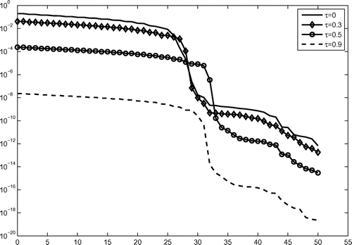
The result of approximate singular values of the solution operator obtained by our method described in Section 2.1 for different $\mathit{\tau }$ are given in Figure 1. From these singular values we see that our inverse problem is severely ill-posed and the ill-posedness depends on the time interval of observations: the less observation time is, the more ill-posed the problem is.

Figure 1. Singular values: three observations and various time intervals of observations.

Now we show numerical results for reconstructing different initial conditions with different time intervals of observations and different positions for observations.

Example 1:

We set the exact solution to (3.1(3.1) $$\begin{array}{c}\hfill \left\{\begin{array}{c}{u}_t-{(a(x,t)u_x)}_x+b(x,t)u=f(x,t)\text{in}Q,\hfill \\ u(0,t)=u(1,t)=0,t\in (0,T],\hfill \\ u(x,0)=v(x)\text{in}\mathrm{\Omega }.\hfill \end{array}\right.\end{array}$$(3.1) ) $u_{\text{exact}}=e^{t}sin(2\mathit{\pi }x)$. Hence, the exact initial condition is given by $v(x)=sin(2\mathit{\pi }x)$, and the right-hand side $f(x,t)=(1+4{\mathit{\pi }}^2(x^{2}t+2xt+1))e^{t}sin(2\mathit{\pi }x)-2\mathit{\pi }{e}^t(2xt+2t)cos(2\mathit{\pi }x)$. Then a priori estimate $v^{\ast }=1/2$, $\mathit{\tau }=0$, the regularization parameter is chosen to be $\mathit{\gamma }=5\times {10}^{-3}$. The first iteration of the CG method $v^0=0$.

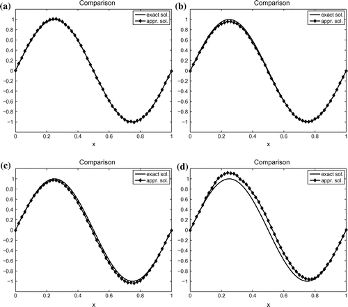
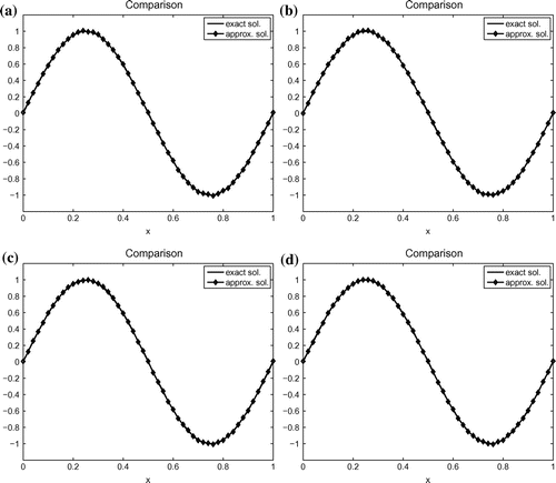
The reconstruction result and the exact initial condition v for various positions of observations are shown in Figure 2. The numerical results show that the quality of the reconstruction depends on the position of observations, the result is better when observations distribute uniformly in $\mathrm{\Omega }$.

 

Figure 2. Example 1: Reconstruction results for (a) 3 uniform observation points in (0, 0.5), error in $L^2$-norm $=0.006116$; (b) 3 uniform observation points in (0.5, 1), error in $L^2$-norm $=0.006133$; (c) 3 uniform observation points in (0.25, 0.75), the error in $L^2$-norm $=0.0060894$; (d) 3 uniform observation points in $\mathrm{\Omega }$, the error in $L^2$-norm $=0.0057764$ .

Example 2:

In this example, the initial condition is chosen to be the same as Example 1, $v^{\ast }=1/2$, and regularization parameter is also $\mathit{\gamma }=5\times {10}^{-3}$, but the starting time for observation is taken to be $\mathit{\tau }=0.01,\mathit{\tau }=0.05,\mathit{\tau }=0.1$ and $\mathit{\tau }=0.3$. The comparison of reconstruction results is displayed in Figure 3.

Table 1 shows the relation between the starting point of observation $\mathit{\tau }$ and the error in the $L^2$-norm of the algorithm when the number of observations is $N=3$ and the regularization parameter is $\mathit{\gamma }=5\times {10}^{-3}$.

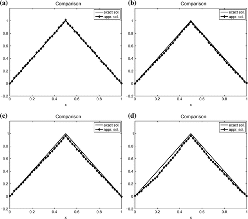
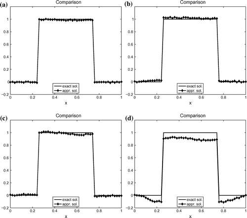
We now test the algorithm for nonsmooth initial conditions. In Examples 3 and 4, we choose v, set $f=0$, and solve the direct problem by the Crank–Nicholson method to find an approximation to the exact solution u, then use these data for reconstructing the exact initial condition v. Here, we use different mesh-sizes for the direct solvers to avoid ‘inverse crime’.

 

Figure 3. Reconstruction result of Example 2: (a) $\mathit{\tau }=0.01$; (b) $\mathit{\tau }=0.05$; (c) $\mathit{\tau }=0.1$; (d) $\mathit{\tau }=0.3$.

Table 1. Example 2: Behaviour of the algorithm with different starting points of observation $\mathit{\tau }$.

Starting point $\mathit{\tau }$	Error in $L^2$ norm
$\mathit{\tau }=0.01$	0.0084225
$\mathit{\tau }=0.05$	0.0226540
$\mathit{\tau }=0.1$	0.0388760
$\mathit{\tau }=0.15$	0.0405540
$\mathit{\tau }=0.2$	0.0622210
$\mathit{\tau }=0.3$	0.1015000
$\mathit{\tau }=0.5$	0.1798100

Note: Number of observations $N=3$; regularization parameter $\mathit{\gamma }=5\times {10}^{-3}$.

Example 3:

In this example, the initial condition is given by$$\begin{array}{c}\hfill v(x)=\left\{\begin{array}{c}2x,\&\text{if}x\le 0.5,\hfill \\ 2(1-x),\&\text{otherwise},\hfill \end{array}\right.\end{array}$$

and $v^{\ast }=1/2$. The regularization parameter and the starting time $\mathit{\tau }$ are chosen to be the same as Example 1. The comparison of reconstruction results is displayed in Figure 4.

 

Figure 4. Reconstruction result of Example 3: (a) $\mathit{\tau }=0.01$; (b) $\mathit{\tau }=0.05$; (c) $\mathit{\tau }=0.1$; (d) $\mathit{\tau }=0.3$.

Example 4:

In this example, the initial condition is given by$$\begin{array}{c}\hfill v(x)=\left\{\begin{array}{c}1,\&\text{if}0.25\le x\le 0.75,\hfill \\ 0,\&\text{otherwise},\hfill \end{array}\right.\end{array}$$

and $v^{\ast }=1/2$. The regularization parameter and the starting time $\mathit{\tau }$ are chosen to be the same as Example 1. The comparison of reconstruction results is displayed in Figure 5.

 

Figure 5. Reconstruction result of Example 4: (a) $\mathit{\tau }=0.01$ ; (b) $\mathit{\tau }=0.05$; (c) $\mathit{\tau }=0.1$; (d) $\mathit{\tau }=0.3$.

3.2. Two-dimensional numerical examples

Set $\mathrm{\Omega }=(0,1)\times (0,1),T=1$. Set further $x=(x_1,x_2)$. The problem Dirichlet problem has the form(3.3) $$\begin{array}{c}\hfill \left\{\begin{array}{c}{u}_t-{(a_1(x_1,x_2,t)u_{x_1})}_{x_1}-{(a_2(x_1,x_2,t)u_{x_2})}_{x_2}+b(x_1,x_2,t)u=f(x_1,x_2,t)\text{in}Q,\hfill \\ u(x_1,0,t)=u(x_1,1,t)=u(0,x_2,t)=u(1,x_2,t)=0,0\le x_1,x_2\le 1,t\in (0,T],\hfill \\ u(x_1,x_2,0)=v(x_1,x_2)\text{in}\mathrm{\Omega }.\hfill \end{array}\right.\end{array}$$(3.3)

For the tests we take $a_1(x,t)=a_2(x,t)=0.5[1-\frac{1}{2}(1-t)cos(3\mathit{\pi }{x}_1)cos(3\mathit{\pi }{x}_2)]$ and $b(x,t)=x_1^2+x_2^2+2x_{1}t+1$.

For discretization, we take the grid sizes 0.02 and the random noise 0.01. The weight functions ${\mathit{\omega }}_i(x)$ are chosen as follows(3.4) $$\begin{array}{c}\hfill {\mathit{\omega }}_i(x)=\left\{\begin{array}{cc}\frac{1}{2\mathit{ϵ}}\hfill & \text{if}x\in (x_1^i-\mathit{ϵ},x_1^i+\mathit{ϵ})\times (x_2^i-\mathit{ϵ},x_2^i+\mathit{ϵ})\hfill \\ 0\hfill & \text{otherwise}\hfill \end{array}\right.\text{with}\mathit{ϵ}=0.01.\end{array}$$(3.4)

As said in the introduction the operators $l_i$ defined by (1.9(1.9) $$\begin{array}{c}\hfill l_{i}u(x,t)={\int }_{\mathrm{\Omega }}{\mathit{\omega }}_i(x)u(x,t)\mathrm{d}x=h_i(t),t\in (\mathit{\tau },T),i=1,\cdots ,N.\end{array}$$(1.9) ) with these weight functions can be regarded as ‘practical’ point-wise observations. We shall test our algorithm for different distributions of $x^i$: they will be taken either in the whole $\mathrm{\Omega }$ or in a part of it: $(0,0.5)\times (0,0.5)$, $(0.5,1)\times (0,0.5)$, $(0.5,1)\times (0.5,1)$ or $(0,0.5)\times (0.5,1)$. The number of observation N will be taken either 4 or 9.

 

Figure 6. Example 5. Reconstruction results: (a) Exact initial condition v; (b) reconstruction of v; (c) point-wise error; (d) the comparison of ${v|}_{x_1=1/2}|$ and its reconstruction.

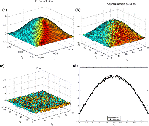
Table 2. Example 5: Behaviour of the algorithm when the number of observations and the positions of observations vary.

Observation region	Iteration	Error in $L^2$ norm
$(0,0.5)\times (0,0.5)$	17	0.028807
$(0.5,1)\times (0,0.5)$	15	0.028366
$(0.5,1)\times (0.5,1)$	15	0.028147
$(0,0.5)\times (0.5,1)$	17	0.028395
$(0,1)\times (0,1)$	17	0.027934

Note: Number of observations $N=4$; regularization parameter $\mathit{\gamma }=5\times {10}^{-3}$.

Table 3. Example 5: Behaviour of the algorithm when the number of observations and the positions of observations vary.

Observation region	Iteration	Error in $L^2$ norm
$(0,0.5)\times (0,0.5)$	29	0.024127
$(0.5,1)\times (0,0.5)$	25	0.024503
$(0.5,1)\times (0.5,1)$	32	0.024667
$(0,0.5)\times (0.5,1)$	25	0.025325
$(0,1)\times (0,1)$	22	0.023887

Note: Number of observations $N=9$; regularization parameter $\mathit{\gamma }=5\times {10}^{-3}$.

Figure 7. Example 6. Reconstruction results: (a) Exact initial condition v; (b) reconstruction of v; (c) point-wise error; (d) the comparison of ${v|}_{x_1=1/2}|$ and its reconstruction.

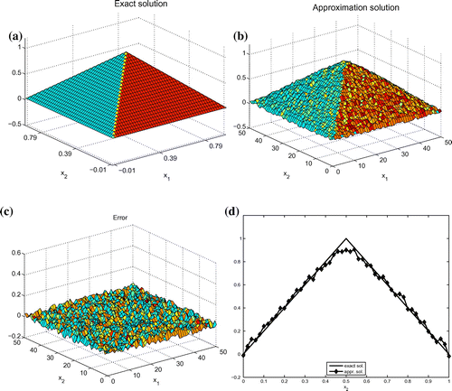
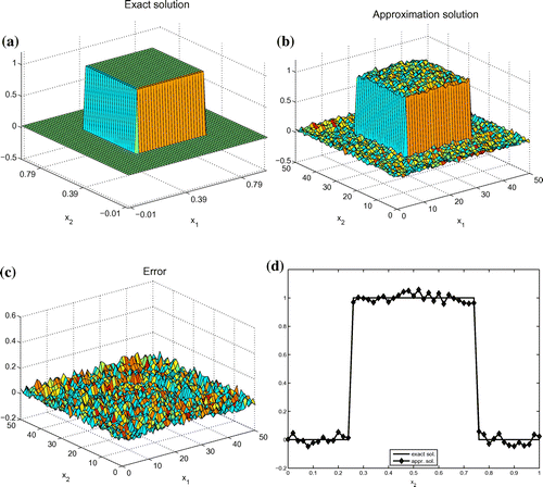
Figure 8. Example 7. Reconstruction results: (a) Exact initial condition v; (b) reconstruction of v; (c) point-wise error; (d) the comparison of ${v|}_{x_1=1/2}|$ and its reconstruction.

Example 5:

We test algorithm for the smooth initial condition given by $v(x)=sin(\mathit{\pi }{x}_1)sin(\mathit{\pi }{x}_2)$ and $u(x,t)=(1-t)v(x)$. The source term f is thus given by$$\begin{array}{cc}& f(x,t)\hfill \\ \hfill & =-v(x)(1-(1-t)\left({\mathit{\pi }}^2+0.5{\mathit{\pi }}^{2}cos(3\mathit{\pi }{x}_1)cos(3\mathit{\pi }{x}_2)-(x_1^2+x_2^2+2x_{1}t+1)\right))\hfill \\ \hfill & +0.75{\mathit{\pi }}^2{(1-t)}^2(sin(3\mathit{\pi }{x}_1)cos(3\mathit{\pi }{x}_2)cos(\mathit{\pi }{x}_1)sin(\mathit{\pi }{x}_2)\hfill \\ \hfill & +cos(3\mathit{\pi }{x}_1)sin(3\mathit{\pi }{x}_2)sin(\mathit{\pi }{x}_1)cos(\mathit{\pi }{x}_2)).\hfill \end{array}$$

The measurement is taken at 9 points, the regularization parameter is set to be $\mathit{\gamma }=5\times {10}^{-3}$. We test the algorithm with the guess $v^{\ast }=1/2$. The reconstruction result and the exact initial condition v are shown in Figure 6. The algorithm stops after 38 iterations and computational time is 87.496271 s and the error in $L^2$-norm is 0.02346. The behaviour of the algorithm when observation regions and number of observations vary is shown in Tables 2 and 3. We can see that the more number of observations we take, the more accuracy we have.

Now we test the algorithm for nonsmooth initial conditions. In Examples 6 and 7, we choose v and set $f=0$, then use the splitting method to find an approximation to the solution u. After that we use the obtained data to test our algorithm.

Example 6:

In this example, we choose 9 observations, set the regularization parameter $\mathit{\gamma }=5\times {10}^{-3}$ and v a multi-linear function given by$$v(x)=\left\{\begin{array}{c}2x_2\text{if}{x}_2\le 1/2\text{and}{x}_2\le x_1\text{and}{x}_1\le 1-x_2,\hfill \\ 2(1-x_2)\text{if}{x}_2\ge 1/2\text{and}{x}_2\ge x_1\text{and}{x}_1\ge 1-x_2,\hfill \\ 2x_1\text{if}{x}_1\le 1/2\text{and}{x}_1\le x_2\text{and}{x}_2\le 1-x_1,\hfill \\ 2(1-x_1)\text{otherwise}\hfill \end{array}\right.$$

and $v^{\ast }=1/2$. The reconstruction results and the exact initial condition v are shown in Figure 7. The algorithm stops after 45 iterations and the computational time is 103.394200 s and the error in $L^2$-norm is 0.024959 .

Example 7:

We test the algorithm with the piecewise constant initial condition$$v(x)=\left\{\begin{array}{c}1\text{if}1/4\le x_1\le 3/4\text{and}1/4\le x_2\le 3/4,\hfill \\ 0\text{otherwise}\hfill \end{array}\right.$$

and $v^{\ast }=1/2$. The algorithm stops after 100 iterations and the computational time is 109.423362 s and the error in $L^2$-norm is 0.033148 (see Figure 8).

Acknowledgements

The constructive comments of the reviewers are kindly acknowledged.

Additional information

Funding

This research was supported by Vietnam National Foundation for Science and Technology Development (NAFOSTED) [grant number 101.02-2014.54].

Notes

No potential conflict of interest was reported by the authors.

References

- Agoshkov VI. Optimal control methods and the method of adjoint equations in problems of mathematical physics. Moscow: Russian Academy of Sciences, Institute for Numerical Mathematics; 2003. 257pp. Russian.
- Shutyaev VP. Control operators and iterative algorithms in variational data assimilation problems. Moscow: Nauka; 2001. 240pp. Russian.
- Aubert G, Kornprobst P. Mathematical problems in image processing. New York (NY): Springer; 2006.
- Hào DN. Methods for inverse heat conduction problems. Frankfurt/Main, Bern, New York (NY), Paris: Peter Lang Verlag; 1998.
- Boussetila N, Rebbani F. Optimal regularization method for ill-posed Cauchy problems. Electron. J. Differ. Equ. 2006;147:1–15.
- Hào DN, Duc NV. Stability results for backward parabolic equations with time dependent coefficients. Inverse Prob. 2011;27:025003, 20pp.
- Li J, Yamamoto M, Zou J. Conditional stability and numerical reconstruction of initial temperature. Commun. Pure Appl. Anal. 2009;8:361–382.
- Tröltzsch F. Optimal control of partial differential equations: theory, methods and applications. Providence (RI): American Mathematical Society; 2010.
- Ladyzhenskaya OA, Solonnikov VA, Ural’ceva NN. Linear and quasilinear equations of parabolic type. Providence (RI): American Mathematical Society; 1968.
- Wloka J. Partial differential equations. Cambridge: Cambridge University Press; 1987.
- Klibanov MV. Carleman estimates for the regularization of ill-posed Cauchy problems. Appl. Numer. Math. 2015;94:46–74.
- Klibanov MV, Kuzhuget AV, Golubnichiy KV. An ill-posed problem for the Black-Scholes equation for a profitable forecast of prices of stock options on real market data. Inverse Prob. 2016;32:015010, 16pp.
- Oanh NTN. A splitting method for a backward parabolic equation with time-dependent coefficients. Comput. Math. Appl. 2013;65:17–28.
- Trefethen LN, Bau D III. Numerical linear algebra. Philadelphia: SIAM; 1997.
- Hào DN, Oanh NTN. Determination of the initial condition in parabolic equations from boundary observations. J. Inverse Ill-Posed Prob. 2016;24:195–220.
- Nocedal J, Wright SJ. Numerical optimization. 2nd ed. New York (NY): Springer; 2006.
- Hinze M. A variational discretization concept in control constrained optimization: the linear-quadratic case. Comput. Optimiz. Appl. 2005;30:45–61.
- Marchuk GI. Methods of numerical mathematics. New York (NY): Springer-Verlag; 1975.
- Marchuk GI. Splitting and alternating direction methods. In Ciarlet PG, Lions JL, editors. Handbook of numerical mathematics. Volume 1: finite difference methods. North-Holland, Amsterdam: Elsevier Science Publisher B.V.; 1990.
- Yanenko NN. The method of fractional steps. Berlin: Springer-Verlag; 1971.
- Hào DN, Thành NT, Sahli H. Splitting-based gradient method for multi-dimensional inverse conduction problems. J. Comput. Appl. Math. 2009;232:361–377.
- Oanh NTN, Huong BV. Determination of a time-dependent term in the right hand side of linear parabolic equations. Acta Math. Vietnam. 2016;41:313–335.
- Thành NT. Infrared thermography for the detection and characterization of buried objects [PhD thesis]. Brussels, Belgium: Vrije Universiteit Brussel; 2007.
- Ladyzhenskaya OA. The boundary value problems of mathematical physics. New York (NY): Springer-Verlag; 1985.
- Hào DN, Thanh PX, Lesnic D, Johansson BT. A boundary element method for a multi-dimensional inverse heat conduction problem. Int. J. Comput. Math. 2012;89:1540–1554.
- Hào DN. A noncharacteristic Cauchy problem for linear parabolic equations II: a variational method. Numer. Funct. Anal. Optim. 1992;13:541–564.
- Hào DN. A noncharacteristic Cauchy problem for linear parabolic equations III: a variational method and its approximation schemes. Numer. Funct. Anal. Optim. 1992;13:565–583.
- Nemirovskii AS. The regularizing properties of the adjoint gradient method in ill-posed problems. Zh. vychisl. Mat. Mat. Fiz. 1986;26:332–347; Engl. Transl. in U.S.S.R. Comput. Maths. Math. Phys. 1986;26:7–16.