A simple spatial integration scheme for solving Cauchy problems of non-linear evolution equations

Abstract

In this study, we address a new and simple non-iterative method to solve Cauchy problems of non-linear evolution equations without initial data. To start with, these ill-posed problems are analysed by utilizing a semi-discretization numerical scheme. Then, the resulting ordinary differential equations at the discretized times are numerically integrated towards the spatial direction by the group-preserving scheme (GPS). After that, we apply a two-stage GPS to integrate the semi-discretized equations. We reveal that the accuracy and stability of the new approach is very good from several numerical experiments even under a large random noisy effect and a very large time span.

Keywords:

• Non-linear evolution equation
• severely ill-posed problem
• Cauchy problem
• group preserving scheme (GPS)
• without initial condition

1. Introduction

Non-linear evolution equations have a very important role in several scientific and engineering fields. These equations appear in heat conduction, fluid dynamics, gas dynamics, number theory, elasticity and so forth. There are several well-known equations of this class: the Burgers equation, Fisher equation, Huxley equation, generalized Burgers–Huxley equation (GBHE), generalized Burgers–Fisher equation (GBFE), generalized Fitzhugh-Nagumo equation (GFNE) and Newell–Whitehead–Segel equation (NWSE). In 1987, the GBHE was investigated by Satsumac [1]. The GBHE and GBFE can be regarded as two different models to describe the interaction between the reaction mechanisms, convection effects and diffusion transports, respectively. Generally speaking, the exact solutions of non-linear evolution equations are difficult to reveal and often impossible to be obtained. Thus, the numerical methods are recommended to make keen observation of the non-linear models. The traditional methods are available for the numerical solution of the differential equations by using the finite difference method (FDM), finite element method (FEM) and finite volume method (FVM) and so forth. The FDM has lost its popularity because of stability problems. The FEM and FVM that require more mesh generations in higher dimensions are tough tasks in the computational process.

For the approximation, analytical and exact methods of GBHE, GBFE, GFNE and NWSE, Wang et al. [2] have discussed the exact solitary wave solutions of the GBHE by utilizing the relevant non-linear transformation. They claimed that this approach can also be applied to the GBFE. Later, Wazwaz [3] derived the travelling wave solutions for the Burgers, Fisher, Huxley equations and the combined forms of these equations. The tanh-coth method is used to decide these sets of travelling wave solutions. The kinks and periodic wave solutions are established. Deng [4] used the first-integral method to solve the GBHE and obtained a class of travelling solitary wave solutions, of which the approach was based on the ring theory of commutative algebra. After that, Babolian and Saeidian [5] revealed that the homotopy analysis method (HAM) can be used to obtain the analytic approximate solutions of Burgers, Fisher, Huxley, Burgers-Fisher and GBHEs. Then, Molabahrami and Khani [6] also employed the HAM to deal with the BHE and provided a simple way to adjust and control the convergence region of solution series. Later, Deng et al. [7] proposed the first-integral method to resolve the GBHE with non-linear terms of any order and attained some exact explicit travelling wave solutions. Gao and Zhao [8] utilized the He’s Exp-function method to obtain a series of new exact solutions of the GBHE. They announced that this approach was straightforward and concise. After that, Zhou et al. [9] investigated the bounded travelling waves of the BHE and discussed the bifurcations of codimension 1 and 2 types. By reduction to the centre manifolds and normal forms, they gave the conditions for the appearance of homoclinic solutions, heteroclinic solutions and periodic solutions, which correspondingly gave the conditions for the existence of solitary waves, kink waves and periodic waves, which are three basic types of bounded travelling waves. Then, Krisnangkura et al. [10] employed the standard tanh method to resolve the GBHE and obtained the exact travelling wave solutions which occurred in the description of many non-linear wave phenomena. Later, Chen and Zhang [11] discussed the GBFE and the Kuramoto-Sivashinsky equation by utilizing a generalized tanh function method. The main idea of this scheme is to take full advantage of the Riccati equation which has more new solutions. Ismail et al. [12] proposed the Adomian decomposition method (ADM) to solve the BHE and BFE and attained approximation solutions. After that, Wazwaz [13,14] also used standard tanh method to resolve and to cope with the generalized forms of KdV, non-linear heat conduction and BFE. The present study focuses on the case where the parameter M is a noninteger. Wazwaz [13,14] derived a variety of exact travelling wave solutions of distinct physical structures. This scheme can be employed in a variety of many types non-linearity. Later, El-Wakil and Abdou [15] proposed the modified extended tanh-function method to solve Zakharov–Kuznetsov–Benjamin–Bona–Mahony equation, Fisher-type equation, GBFE and Drinfeld–Sokolov system. They claimed that the algorithm was simpler than other conventional approaches. About the GFNE, it has diverse applications in the areas of nuclear reactor theory, antocatalytic chemical reaction, branching Brownian motion, neurophysiology, logistic population growth and flame propagation [16–21]. For the NWSE, Aasaraai [22] applied the differential transform method (DTM) to cope with this equation and acquired the analytic solution. Moreover, it is found in Ref. [22] that DTM has the advantage of without using Adomian’s polynomials.

For the numerical approaches of GBHE, GBFE, GFNE and NWSE, Batiha et al. [23] compared the numerical results of generalized Huxley equation (GHE) of He’s variational iteration method (VIM) with ADM, and found that the former was more effective than the later. Then, Hashemi et al. [24] analysed the He’s homotopy perturbation method of the GHE and revealed that their approach was more effective than the ADM. It is also found in Ref. [24] that the proposed scheme overcomes the difficulties arising in calculating Adomian polynomials. Later, Darvishi et al. [25] addressed the spectral collocation method and Darvishi’s preconditionings to solve the GBHE and small numerical errors were obtained. Khattak [26] employed Kansa’s collocation method (Radial basis functions method) to resolve the GBHE, which compared with the exact solution, the VIM and ADM in order to illustrate the efficiency of the proposed approach. After that, Macías-Díaz et al. [27] used a non-standard, finite-difference algorithm to approximate the solutions of a GBHE form fluid dynamic. Their numerical method preserved the skew-symmetry of the partial differential equation (PDE) under study and, under some analytical constraints of the model constants and the computational parameters involved; therefore, it was able to preserve the boundedness and the positivity of the solutions. In the linear regime, the method is consistent to first order in time (due partially to the inclusion of a tuning parameter in the approximation of a temporal derivative), and to second order in space. Subsequent to Ref. [27], Zhang et al. [28] presented the local discontinuous Galerkin method to cope with the GBHE and GBFE, and the numerical results attained by this way were compared with the exact solution to demonstrate the accuracy and capability of this approach. After that, Çelik [29] demonstrated the Haar wavelet method to obtain good results, by which he claimed that the method was a very reliable, simple, small computation costs, flexible, and convenient alternative approach. Then, Dehghan et al. [30] utilized two numerical techniques on the basis of the interpolating scaling functions and the mixed collocation finite difference schemes to solve the GBHE. Ervin et al. [31] showed a finite element algorithm capable of preserving the nonnegative and bounded solutions of the GBHE. A priori error estimate for the approximation was also derived, and several numerical experiments were presented which supported the derived theoretical results. Later, a lattice Boltzmann model was employed by Duan et al. [32] to cope with the GBHE. By choosing the proper time and space scales and applying the Chapman–Enskog expansion, the governing equation was recovered correctly from the lattice Boltzmann equation, and the local equilibrium distribution functions were attained. After that, Kaya and El-Sayed [33] considered the decomposition scheme and attained the exact solutions of the GBFE for the initial condition without using any classical transformations and then its numerical solutions were constructed without using any discretization technique. Later, Zhu and Kang [34] developed the cubic B-spline quasi-interpolation to solve the BFE; moreover, the numerical scheme was presented, by using the derivative of the quasi-interpolation to approximate the spatial derivative of the dependent variable and a low order forward difference to approximate the time derivative of the dependent variable. They announced that the main advantage of the resulting approach was that the method was very simple and easy to implement. Then, Javidi [35] proposed a Chebyshev spectral collocation domain decomposition (DD) semi-discretization and a grid mapping to cope with the GBHE. Besides, the application of this modified approach to the GBHE shows that this scheme is faster and more accurate than the standard Chebyshev spectral collocation DD method. After that, Soheili et al. [36] utilized a moving mesh partial differential equation approach to obtain good results; however, this method was complicated. Zhao et al. [37] employed the pseudo-spectral method to obtain approximation of GBFE. For the time discretization they apply Crank–Nicolson/leapfrog scheme. The space discretization is based on Legendre Galerkin formulation while the Chebyshev–Gauss–Lobatto nodes are used in practical computation, which is called ‘Chebyshev–Legendre’ method. After that, the results obtained by a modified lattice Boltzmann scheme used by Xiang et al. [38] agree well with the analytical solution. This means that the proposed method under the best choice of the parameters can preserve the better stability and higher accuracy in comparison with previous schemes. For the GFNE, Bhrawy [39] addressed a Jacobi-Gauss-Lobatto collocation method to deal with this equation with time-dependent coefficients and attained accurate results. Later, Jiwari et al. [40] applied the polynomial differential quadrature method to solve the GFNE with time-dependent coefficients. The accuracy and efficiency of the proposed approach is shown by three numerical examples. For the NWSE, several algorithms were proposed to solve the non-linear PDE, e.g. the homotopy perturbation method [41], the ADM and multiquadric quasi-interpolation method [42], the non-standard symmetry-preserving method [43], the Laplace ADM [44], the reduced DTM and the ADM [45], the homotopy perturbation algorithm [46], and the cubic B-spline quasi-interpolation [47]. Nevertheless, the above-mentioned researches did not discuss how the initial data were disturbed by noise, multi-dimensional problems and the complex geometry. In the engineering fields, we often encounter the noisy initial conditions and boundary conditions rather than the ideal conditions of the above-mentioned literature.

For the Cauchy inverse problem of GBHE, GBFE, GFNE and NWSE, to the authors’ best knowledge, there is no published report showing that the numerical methods for these severely Cauchy problems can provide accurate results. Therefore, our approach is combined with the group-preserving scheme (GPS) proposed by Liu [48], which can preserve the Lie-symmetry SO_o (n, 1), of the augmented dynamical system. Later, Lee and Liu [49] have extended the first-order GPS to the fourth-order GPS. In fact, the GPS is very effective to cope with the ordinary differential equations (ODEs) as displayed by Liu [50] for stiff ODEs, and by Liu [51] for ODEs with constraints. Chen et al. [52] have modified the GPS to a time step size adaptive numerical method for ODEs. Some extensions of the GPS to other fields were undertaken by Liu [53–59], Liu et al. [60–63], Chang et al. [64–69], Liu and Chang [70,71]. Moreover, Liu and Chang [72] proposed a simple approach to solve the inverse Cauchy problem of non-linear heat equation without initial value. In this article, we reveal that our proposed scheme is easier than that proposed by Liu and Chang [72].

The remainder of this study is organized as follows. Section 2 interprets a formulation of the problem and a spatial integration method. Moreover, we propose a numerical algorithm to solve the inverse Cauchy problems of non-linear evolution equations without initial data, which are discretized into a non-linear ODEs system by employing the numerical scheme of lines. Eight numerical examples are presented in Section 3 to validate the performance of the newly developed two-stage group preserving scheme. Finally, some conclusions are shown in Section 4.

2. Problem statement and a spatial integration method

We numerically tackle a mixed type inverse Cauchy problem, and the retrieval of initial condition for a non-linear one-dimensional evolution equation:(1) $$u_{xx}(x,t)=u_t(x,t)-H(x,t,u^p,u_x),0<x<\ell ,0<t<T,$$(1) (2) $$u(0,t)=u_0(t)\text{,}$$(2) (3) $$u_x(0,t)=q_0(t),$$(3)

where u indicates a scalar physical quantity, ℓ stands for the length of thin and long rod, T denotes the terminal time, $H(x,t,u^p,u_x)$ represents the source term, p is a positive integer, u₀ means the physical quantity on the left-end boundary condition, and q₀ signifies the physical flux on the left-end boundary condition.

To tackle the above ill-posed problem, we can apply a semi-discretization of time variable, and directly utilize a numerical integration scheme to the discretized equations along the x-axis. The integration direction is along the x-axis from x = 0 to x = ℓ. In this article, we resolve this inverse problem through a two-stage GPS.

2.1. A semi-discretization

The numerical approach of lines is easy to implement for a given system of PDEs. The semi-discrete process produces a coupled system of ODEs which are being numerically integrated. For Equation (1(1) $$u_{xx}(x,t)=u_t(x,t)-H(x,t,u^p,u_x),0<x<\ell ,0<t<T,$$(1) ), we employ the numerical approach of lines to discretize the time coordinate t and maintain x a continuous variable, in which t_i = (i−1)Δt = (i−1)t_f/(m−1) is a uniform time step size, such that we can acquire(4) $$\frac{\mathit{\partial }{u}_i(x)}{\mathit{\partial }x}=v_i(x),i=\text{1},\dots ,m,$$(4) $$\frac{\mathit{\partial }{v}_i(x)}{\mathit{\partial }x}=\frac{u_{i+1}-u_{i-1}}{2\mathrm{\Delta }t}-H_i,i=\text{2},\dots ,m-1,$$$$\frac{\mathit{\partial }{v}_1(x)}{\mathit{\partial }x}=-\frac{3u_1-4u_2+u_3}{2\mathrm{\Delta }t}-H_1,i=\text{1},$$

(5) $$\frac{\mathit{\partial }{v}_m(x)}{\mathit{\partial }x}=\frac{3u_m-4u_{m-1}+u_{m-2}}{2\mathrm{\Delta }t}-H_m,i=m,$$(5)

where for simple notation we apply H_i to indicate $H(x,t,u^p,u_x)$ at time t_i.

In our approach of problem (1)–(3) by a semi-discretization with respect to t, we obtain a system of ODEs with Equations (2(2) $$u(0,t)=u_0(t)\text{,}$$(2) ) and (3(3) $$u_x(0,t)=q_0(t),$$(3) ) being the initial conditions, which are supposed to be bounded functions. For the resulting vector fields, we suppose that they are Lipschitz continuous with respect to u, such that the solutions of the ODEs are existent. Even under this very weak-topology, the problem is highly ill-posed.

2.2. Group-preserving scheme

GPS can preserve the internal symmetry group of the considered system. For non-linear differential equations systems, Liu [48] has embedded them into the augmented dynamical systems, which concern with not only the evolution of state variables but also the evolution of the magnitude of state variables vector. That is, for an n ODEs system:(6) $$\dot{\mathbf{x}}=\mathbf{f}(\mathbf{x},t),\mathbf{x}\in {\mathcal{R}}^n,t\in {\mathcal{R}}^{+},$$(6)

we can embed it into the following n + 1-dimensional augmented dynamical system:(7) $$\frac{\text{d}}{\text{d}t}\left[\begin{array}{c}\mathbf{x}\\ ∥\mathbf{x}∥\end{array}\right]=\left[\begin{array}{cc}{\mathbf{0}}_{n\times n}& \frac{\mathbf{f}(\mathbf{x},t)}{∥\mathbf{x}∥}\\ \frac{{\mathbf{f}}^T(\mathbf{x},t)}{∥\mathbf{x}∥}& 0\end{array}\right]\left[\begin{array}{c}\mathbf{x}\\ ∥\mathbf{x}∥\end{array}\right].$$(7)

Here, we assume $∥\mathbf{x}∥>0$ and hence, the above system is well-defined.

It is obvious that the first row in Equation (7(7) $$\frac{\text{d}}{\text{d}t}\left[\begin{array}{c}\mathbf{x}\\ ∥\mathbf{x}∥\end{array}\right]=\left[\begin{array}{cc}{\mathbf{0}}_{n\times n}& \frac{\mathbf{f}(\mathbf{x},t)}{∥\mathbf{x}∥}\\ \frac{{\mathbf{f}}^T(\mathbf{x},t)}{∥\mathbf{x}∥}& 0\end{array}\right]\left[\begin{array}{c}\mathbf{x}\\ ∥\mathbf{x}∥\end{array}\right].$$(7) ) is the same as the original Equation (6(6) $$\dot{\mathbf{x}}=\mathbf{f}(\mathbf{x},t),\mathbf{x}\in {\mathcal{R}}^n,t\in {\mathcal{R}}^{+},$$(6) ), but the inclusion of the second row in Equation (7(7) $$\frac{\text{d}}{\text{d}t}\left[\begin{array}{c}\mathbf{x}\\ ∥\mathbf{x}∥\end{array}\right]=\left[\begin{array}{cc}{\mathbf{0}}_{n\times n}& \frac{\mathbf{f}(\mathbf{x},t)}{∥\mathbf{x}∥}\\ \frac{{\mathbf{f}}^T(\mathbf{x},t)}{∥\mathbf{x}∥}& 0\end{array}\right]\left[\begin{array}{c}\mathbf{x}\\ ∥\mathbf{x}∥\end{array}\right].$$(7) ) gives us a Minkowskian structure of the augmented state variables of $\mathbf{X}\text{:}={({\mathbf{x}}^T,∥\mathbf{x}∥)}^T$ satisfying a future cone condition:(8) $${\mathbf{X}}^T\mathbf{g}\mathbf{X}=0,$$(8)

where(9) $$\mathbf{g}=\left[\begin{array}{cc}{\mathbf{I}}_n& {\mathbf{0}}_{n\times 1}\\ {\mathbf{0}}_{1\times n}& -1\end{array}\right]$$(9)

is a Minkowski metric. ${\mathbf{I}}_n$ is the identity matrix of order n, and the superscript T denotes the transpose. In terms of $({\mathbf{x}}^T,∥\mathbf{x}∥),$ Equation (8(8) $${\mathbf{X}}^T\mathbf{g}\mathbf{X}=0,$$(8) ) holds, as(10) $${\mathbf{X}}^T\mathbf{g}\mathbf{X}=\mathbf{x}·\mathbf{x}-{∥\mathbf{x}∥}^2={∥\mathbf{x}∥}^2-{∥\mathbf{x}∥}^2=0,$$(10)

where the dot between two n-dimensional vectors represents their Euclidean inner product. The cone condition is thus the most natural constraint that we can impose on the dynamical system (7).

Consequently, we have an n + 1-dimensional augmented system:(11) $$\dot{\mathbf{X}}=\mathbf{AX}$$(11)

with a constraint (8), where(12) $$\mathbf{A}:=\left[\begin{array}{cc}{\mathbf{0}}_{n\times n}& \frac{\mathbf{f}(\mathbf{x},t)}{∥\mathbf{x}∥}\\ \frac{{\mathbf{f}}^T(\mathbf{x},t)}{∥\mathbf{x}∥}& 0\end{array}\right]$$(12)

is an element of the Lie algebra so(n, 1) of the proper orthochronous Lorentz group SO_o(n,1), satisfying(13) $${\mathbf{A}}^T\mathbf{g}+\mathbf{g}\mathbf{A}=\mathbf{0}.$$(13)

This fact prompts us to employ the group preserving scheme, and its discretized mapping G exactly preserves the following properties:(14) $${\mathbf{G}}^T\mathbf{g}\mathbf{G}=\mathbf{g},$$(14) (15) $$\text{det}\mathbf{G}=1,$$(15) (16) $$G_0^0>0,$$(16)

where $G_0^0$ is the 00th component of G. Such G is an element of SO_o(n,1). The term orthochronous should be understood as the preservation of the sign of $∥\mathbf{x}∥>0$.

SO_o(n,1) is a Lie-group, where SO means that it is a special orthogonal matrix with determinant being one in the Minkowski space with a signature (n,1), which means that we have n + 1 and one −1 in the metric tensor g. The subscript _o in SO_o(n,1) means that it is the orthochronous with the property (16).

2.3. Two-stage integration algorithm

First, we integrate Equations (4(4) $$\frac{\mathit{\partial }{u}_i(x)}{\mathit{\partial }x}=v_i(x),i=\text{1},\dots ,m,$$(4) ) and (5(5) $$\frac{\mathit{\partial }{v}_m(x)}{\mathit{\partial }x}=\frac{3u_m-4u_{m-1}+u_{m-2}}{2\mathrm{\Delta }t}-H_m,i=m,$$(5) ) by utilizing the GPS developed by Liu [48], where we indicate the spatial step size by Δx = ℓ/(n−1). In this integration, we can acquire the missing initial conditions which are denoted by u₀(j), j = 2,…, n. Then, under the same left-end boundary conditions and the computed initial conditions u₀(j), j = 2,…, n from the previous stage GPS, we employ the second-stage GPS to integrate the following ODEs:(17) $$\frac{\mathit{\partial }{u}_i(x)}{\mathit{\partial }x}=v_i(x),i=\text{2},\dots ,m,$$(17) $$\frac{\mathit{\partial }{v}_i(x)}{\mathit{\partial }x}=\frac{u_{i+1}-u_{i-1}}{2\mathrm{\Delta }t}-H_i,i=\text{2},\dots ,m-1,$$(18) $$\frac{\mathit{\partial }{v}_m(x)}{\mathit{\partial }x}=\frac{3u_m-4u_{m-1}+u_{m-2}}{2\mathrm{\Delta }t}-H_m,i=m,$$(18)

where we do not require integrating u₁(x_j), which is attained from u₀(j), j = 2,…, n. At the end of the second-stage integration, we can acquire temperature and heat flux at the right-end boundary and the whole domain. Besides, we could construct a geometry (future cone), algebra (Lie algebra) and group (Lie group) description of the ill-posed problems governed by differential equations.

3. Numerical examples

In this section, we examine the methodology of the spatial integration method and the two-stage GPS for some instances. All the required left-end boundary conditions can be derived from exact solution. Here, we deliberate the noisy data being imposed on the two left-end boundary conditions by(19) $${\widehat{u}}_0(t_i)=u_0(t_i)[1+sR(i)],{\widehat{q}}_0(t_i)=q_0(t_i)[1+sR(i)],$$(19)

where R(i) are random numbers in [−1, 1], and s is the intensity of noise.

The root-mean-square-error (RMSE) is defined in the retrievals of the initial condition and the right-end boundary conditions by(20) $$\text{RMSE}1:=\sqrt{\frac{1}{n}\sum _{j=1}^n{\left[u^{\ast }(x_j,0)-u(x_j,0)\right]}^2},$$(20) (21) $$\text{RMSE}2:=\sqrt{\frac{1}{m}\sum _{k=1}^m{\left[u^{\ast }(\ell ,t_k)-u(\ell ,t_k)\right]}^2},$$(21) (22) $$\text{RMSE}3:=\sqrt{\frac{1}{m}\sum _{k=1}^m{\left[u_x^{\ast }(\ell ,t_k)-u_x(\ell ,t_k)\right]}^2},$$(22)

where n is the number of steps and m is the number of the discretized times in the GPS utilized to integrate the governing equations along the x-direction. When u^*(x_j, 0), u^*(ℓ, t_k) and $u_x^{\ast }(\ell ,t_k)$ indicate the numerical solutions, u(x_j, 0), u(ℓ, t_k) and u_x(ℓ, t_k) stand for the exact solutions.

3.1. Example 1

We first deliberate the following Burgers equation [53]:

(23) $$u_{xx}=u_t+u{u}_x+0.5e^{-2t}sin(2x),\text{0}<x<\ell \text{,}0<t<T,$$(23)

and the exact solution u of Equations (2(2) $$u(0,t)=u_0(t)\text{,}$$(2) ), (3(3) $$u_x(0,t)=q_0(t),$$(3) ) and (23(23) $$u_{xx}=u_t+u{u}_x+0.5e^{-2t}sin(2x),\text{0}<x<\ell \text{,}0<t<T,$$(23) ) is given by

(24) $$u(x,t)=cos(x)e^{-t},\text{0}<x<1\text{,}0<t<10.$$(24)

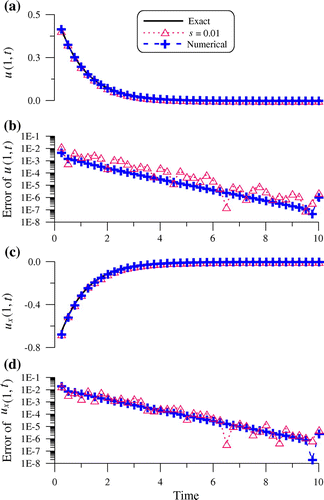
Under the following parameters m = 41, n = 101, T = 10 and under a noise with s = 0.01, we solve the above inverse problem to recover initial condition and two right-end boundary conditions.

In Figures 1 and 2, we compare the recovered initial condition, temperature and heat flux at x = 1 with exact solution, which are very accurate with the maximum error and RMSE1 of initial condition being 3.74 × 10⁻³ and 2.60 × 10⁻³, respectively, and the maximum error and RMSE3 of right-end heat flux are 1.97 × 10⁻² and 3.77 × 10⁻³, respectively. At the same time, we also note that the maximum error and RMSE2 of right-end temperatures are 1.47 × 10⁻² and 2.55 × 10⁻³, respectively. The accuracy as demonstrated in Figure 2 is good in the order of O(10⁻¹)－O(10⁻⁸) even under a moderate noisy effect. Besides, We add Table 2 for this example which show the error in versus the noise s for some values of u_x(1, t) and u(1, t).

Figure 1. For example 1: (a) comparing numerical and exact initial conditions, and (b) the numerical error of initial conditions.

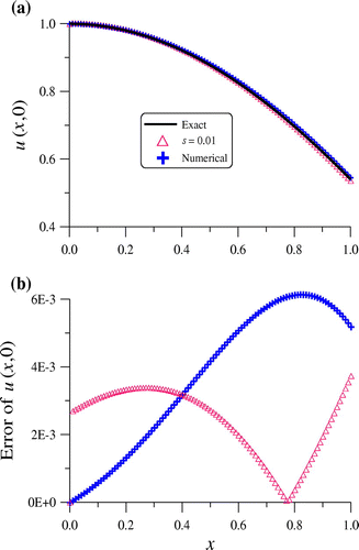
Figure 2. For example 1: (a) comparing numerical and exact right-end temperatures, (b) the numerical error of right-end temperatures, (c) comparing numerical and exact right-end heat fluxes, and (d) the numerical error of right-end heat fluxes.

For the stability analysis of scheme, we define that the stability index r is equal to Δt/(Δx)². Besides, we proceed to investigate the stability of approach in Equation (23(23) $$u_{xx}=u_t+u{u}_x+0.5e^{-2t}sin(2x),\text{0}<x<\ell \text{,}0<t<T,$$(23) ) and find that the range of r for stability is r ≤ 2500. In Table 1, r is recorded with respect to Δx, of which we can see that the admissible range of r.

Table 1. We take example 1 to be an example for the stability analysis of the group-preserving scheme, whose value is r ≤ 2500, and it is related to the grid spacing length vs. the stable index r.

Δx	r
0.5	1
0.2	6.25
0.1	25
0.0625	64
0.05	100
0.04	156.25
0.02	625
0.01	2500

For this example, we obtain the maximum error and RMSE1 for u(x, 0) by increasing in number of n with fixed m and s and report them in Table 3. We also acquire the maximum error and RMSE2 for u(l, t) by increasing in number of m with fixed n and s and report them in Table 4.

3.2. Example 2

Then, we contemplate the following Fisher equation [73]:

(25) $$u_{xx}=u_t-6u(1-u),\text{0}<x<\ell \text{,}0<t<T,$$(25)

and the exact solution u of Equations (2(2) $$u(0,t)=u_0(t)\text{,}$$(2) ), (3(3) $$u_x(0,t)=q_0(t),$$(3) ) and (25(25) $$u_{xx}=u_t-6u(1-u),\text{0}<x<\ell \text{,}0<t<T,$$(25) ) is given by

(26) $$u(x,t)={(1+e^{x-5t})}^{-2},\text{0}<x<1\text{,}0<t<5.$$(26)

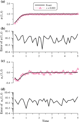
Under the following parameters m = 41, n = 21, T = 5 and under the noises with s = 0.003, we solve the above inverse problem to retrieve initial condition and two right-end boundary conditions. Besides, We add Table 2 for this example which show the error in versus the noise s for some values of u_x(1, t) and u(1, t).

Table 2. We take four test examples to show the error in versus the noise s for some values of u_x(1, t) and u(1, t).

Examples	Error s	RMSE2[u(1, t)]	RMSE3[ux(1, t)]
Example 1	0.001	9.67 × 10^−4	3.59 × 10^−3
	0.005	1.65 × 10^−3	3.43×10^−3
	0.009	2.37 × 10^−3	3.65 × 10^−3
Example 2	0.0008	7.58 × 10^−3	1.51 × 10^−2
	0.001	8.01 × 10^−3	1.71 × 10^−2
	0.002	1.09 × 10^−2	2.87 × 10^−2
Example 3	0.03	1.33 × 10^−2	1.24 × 10^−2
	0.04	1.52 × 10^−2	1.38 × 10^−2
	0.05	1.75 × 10^−2	1.54 × 10^−2
Example 4	0.002	4.94 × 10^−3	8.61 × 10^−3
	0.005	5.91 × 10^−3	8.61 × 10^−3
	0.008	7.75 × 10^−3	8.93 × 10^−3

In Figure 3, we compare the recovered temperature and heat flux at x = 1 with exact solution, which are accurate with the maximum error and RMSE1 of initial condition being 1.48 × 10⁻² and 5.85 × 10⁻³, respectively, and the maximum error and RMSE3 of right-end heat flux are 0.1483 and 4.13 × 10⁻², respectively. At the same time, we also note that the maximum error and RMSE2 of right-end temperatures are 3.92 × 10⁻² and 1.44 × 10⁻², respectively. The accuracy as displayed in Figure 3 is good in the order of O(10⁻¹)－O(10⁻⁴) even under the moderate noisy effect. Furthermore, the proposed scheme does not need to use the regularization technique and still obtains good results.

Figure 3. For example 2: (a) comparing numerical and exact right-end temperatures, (b) the numerical error of right-end temperatures, (c) comparing numerical and exact right-end heat fluxes, and (d) the numerical error of right-end heat fluxes.

For this example, we obtain the maximum error and RMSE1 for u(x, 0) by increasing in number of n with fixed m and s and report them in Table 3. We also acquire the maximum error and RMSE2 for u(l, t) by increasing in number of m with fixed n and s and report them in Table 4.

Table 3. We obtain the maximum error and RMSE1 for u(x, 0) by increasing in number of n with fixed m and s.

Examples	n	RMSE1[u(x, 0)]	Maximum error
Example 1 with fixed m = 41 and s = 0.01	41	4.60 × 10^−3	6.09 × 10^−3
	51	3.79 × 10^−3	5.07 × 10^−3
	81	2.82 × 10^−3	3.75 × 10^−3
Example 2 with fixed m = 41 and s = 0.003	41	6.12 × 10^−3	1.72 × 10^−2
	51	6.15 × 10^−3	1.75 × 10^−2
	81	6.20 × 10^−3	1.80 × 10^−2
Example 3 with fixed m = 41 and s = 0.02	41	3.69 × 10^−2	9.58 × 10^−2
	51	3.51 × 10^−2	9.09 × 10^−2
	81	3.25 × 10^−2	8.36 × 10^−2
Example 4 with fixed m = 41 and s = 0.01	41	1.63 × 10^−2	3.20 × 10^−2
	51	1.62 × 10^−2	3.19 × 10^−2
	81	1.61 × 10^−2	3.18 × 10^−2

Table 4. We obtain the maximum error and RMSE2 for u(1, t) by increasing in number of m with fixed n and s.

Examples	m	RMSE2[u(1, t)]	Maximum error
Example 1	51	2.17 × 10^−3	8.90 × 10^−3
	81	3.07 × 10^−3	1.34 × 10^−2
	101	5.02 × 10^−3	3.66 × 10^−2
Example 2	51	1.84 × 10^−2	0.102
	81	1.72 × 10^−2	5.95 × 10^−2
	101	2.40 × 10^−2	0.133
Example 3	51	4.33 × 10^−2	0.103
	81	4.70 × 10^−2	9.27 × 10^−2
	101	4.66 × 10^−2	9.50 × 10^−2
Example 4	51	1.02 × 10^−2	4.16 × 10^−2
	81	9.40 × 10^−3	3.79 × 10^−2
	101	9.98 × 10^−3	4.19 × 10^−2

3.3. Example 3

Let us further consider the Huxley equation [32]:(27) $$u_{xx}=u_t-u(1-u)(u-1),\text{0}<x<\ell \text{,}0<t<T,$$(27)

and the exact solution u of Equations (2(2) $$u(0,t)=u_0(t)\text{,}$$(2) ), (3(3) $$u_x(0,t)=q_0(t),$$(3) ) and (27(27) $$u_{xx}=u_t-u(1-u)(u-1),\text{0}<x<\ell \text{,}0<t<T,$$(27) ) is given by

(28) $$u(x,t)=0.5+0.5tanh\left[\left(x-t/\sqrt{2}\right)/\left(2\sqrt{2}\right)\right],\text{0}<x<5\text{,}0<t<50.$$(28)

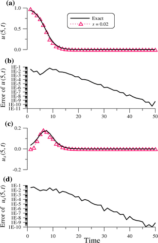
Under the following parameters m = 41, n = 26 and under the noises with s = 0.02, we solve the above inverse problem to recover initial condition and two right-end boundary conditions. Besides, We add Table 2 for this example which show the error in versus the noise s for some values of u_x(1, t) and u(1, t).

In Figure 4, we compare the recovered temperature and heat flux at x = 5 with exact solution, which are accurate with the maximum error and RMSE1 of initial condition being 0.1101 and 4.20 × 10⁻², respectively, and the maximum error and RMSE3 of right-end heat flux are 4.63 × 10⁻² and 1.14 × 10⁻², respectively. At the same time we also note that the maximum error and RMSE2 of right-end temperatures are 5.51 × 10⁻² and 1.19 × 10⁻², respectively. The accuracy as presented in Figure 4 is very good in the order of O(10⁻¹)－O(10⁻¹¹) even under the moderate noisy effect. In addition, to the authors’ best knowledge, there is no report in the literature that the numerical methods for this problem can offer more accurate results than the current one.

Figure 4. For example 3: (a) comparing numerical and exact right-end temperatures, (b) the numerical error of right-end temperatures, (c) comparing numerical and exact right-end heat fluxes, and (d) the numerical error of right-end heat fluxes.

For this example, we obtain the maximum error and RMSE1 for u(x, 0) by increasing in number of n with fixed m and s and report them in Table 3. We also acquire the maximum error and RMSE2 for u(l, t) by increasing in number of m with fixed n and s and report them in Table 4.

3.4. Example 4

Then, let us deliberate the 1-D Burgers–Fisher equation [3]:(29) $$u_{xx}=u_t-u{u}_x-u(1-u),\text{0}<x<\ell \text{,}0<t<T,$$(29)

and the exact solution u of Equations (2(2) $$u(0,t)=u_0(t)\text{,}$$(2) ), (3(3) $$u_x(0,t)=q_0(t),$$(3) ) and (29(29) $$u_{xx}=u_t-u{u}_x-u(1-u),\text{0}<x<\ell \text{,}0<t<T,$$(29) ) is given by

(30) $$u(x,t)=0.5+0.5tanh\left[\left(x+2.5t\right)/\left(2\sqrt{2}\right)\right],\text{0}<x<1\text{,}0<t<50.$$(30)

Under the following parameters m = 41, n = 26, T = 50 and under a noise with s = 0.01, we solve the above inverse problem to recover initial condition and two right-end boundary conditions. Besides, We add Table 2 for this example which show the error in versus the noise s for some values of u_x(1, t) and u(1, t).

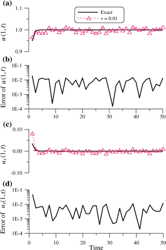
In Figure 5, we compare the recovered temperature and heat flux at x = 1 with exact solution, which are accurate with the maximum error and RMSE1 of initial condition being 3.23 × 10⁻² and 1.65 × 10⁻², respectively, the maximum error and RMSE2 of right-end temperatures are 1.98 × 10⁻² and 9.21 × 10⁻³, respectively, and the maximum error and RMSE3 of right-end heat flux are 4.82 × 10⁻² and 9.31 × 10⁻³, respectively. The accuracy as can be seen from Figure 5 is good in the order of O(10⁻¹)－O(10⁻⁴) even under the moderate noisy effect. To the authors’ best knowledge, there is no published report showing that the numerical methods for this severely ill-posed Cauchy problem can provide more accurate results than the present study.

Figure 5. For example 4: (a) comparing numerical and exact right-end temperatures, (b) the numerical error of right-end temperatures, (c) comparing numerical and exact right-end heat fluxes, and (d) the numerical error of right-end heat fluxes.

For this example, we obtain the maximum error and RMSE1 for u(x, 0) by increasing in number of n with fixed m and s and report them in Table 3. We also acquire the maximum error and RMSE2 for u(l, t) by increasing in number of m with fixed n and s and report them in Table 4.

3.5. Example 5

Let us further contemplate the 1-D GBHE [3]:(31) $$u_{xx}=u_t-u{u}_x-u(1-u)(u-1),\text{0}<x<\ell \text{,}0<t<T,$$(31)

and the exact solution u of Equations (2(2) $$u(0,t)=u_0(t)\text{,}$$(2) ), (3(3) $$u_x(0,t)=q_0(t),$$(3) ) and (31(31) $$u_{xx}=u_t-u{u}_x-u(1-u)(u-1),\text{0}<x<\ell \text{,}0<t<T,$$(31) ) is given by

(32) $$u(x,t)=0.5-0.5tanh\left[(x+1.5t)/4\right],\text{0}<x<1\text{,}0<t<50.$$(32)

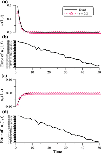
Under the following parameters m = 41, n = 11 and under a noise with s = 0.2, we solve the above inverse problem to recover initial condition and two right-end boundary conditions.

In Figure 6, we compare the recovered temperature and heat flux at x = 1 with exact solution, which are accurate with the maximum error and RMSE1 of initial condition being 2.60 × 10⁻² and 1.65 × 10⁻², respectively, the maximum error and RMSE2 of right-end temperatures are 4.26 × 10⁻² and 6.96 × 10⁻³, respectively, and the maximum error and RMSE3 of right-end heat flux are 8.73 × 10⁻³ and 1.86 × 10⁻³, respectively. The accuracy as can be seen from Figure 6 is very good in the order of O(10⁻¹)－O(10⁻¹⁸) even under the large noisy effect. Nevertheless, to the authors’ best knowledge, there has been no report that numerical approaches can calculate this equation very well as our method.

Figure 6. For example 5: (a) comparing numerical and exact right-end temperatures, (b) the numerical error of right-end temperatures, (c) comparing numerical and exact right-end heat fluxes, and (d) the numerical error of right-end heat fluxes.

3.6. Example 6

Let us consider the 1-D GFNE [39]:(33) $$u_{xx}=u_t-u(1-u)(0.75-u),0<x<\ell \text{,}0<t<T,$$(33)

and the exact solution u of Equations (2(2) $$u(0,t)=u_0(t)\text{,}$$(2) ), (3(3) $$u_x(0,t)=q_0(t),$$(3) ) and (33(33) $$u_{xx}=u_t-u(1-u)(0.75-u),0<x<\ell \text{,}0<t<T,$$(33) ) is given by

(34) $$u(x,t)=0.5+0.5tanh\left[\left(x-\frac{0.5}{\sqrt{2}}t\right)/\left(2\sqrt{2}\right)\right],0<x<4\text{,}0<t<5.$$(34)

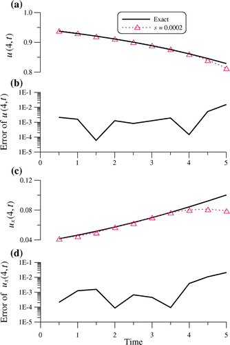
Under the following parameters m = 11, n = 401 and under a noise with s = 2 × 10⁻⁴, we solve the above inverse problem to recover initial condition and two right-end boundary conditions.

In Figure 7, we compare the recovered temperature and heat flux at x = 4 with exact solution, which are very accurate with the maximum error and RMSE1 of initial condition being 2.08 × 10⁻³ and 1.25 × 10⁻³, respectively, the maximum error and RMSE2 of right-end temperatures are 1.52 × 10⁻² and 4.99 × 10⁻³, respectively, and the maximum error and RMSE3 of right-end heat flux are 2.09 × 10⁻² and 7.24 × 10⁻³, respectively. The accuracy as can be seen from Figure 7 is good in the order of O(10⁻¹)－O(10⁻⁵) even under the small noisy effect. Furthermore, we also do not need to employ the regularisation skill and still attain good results.

Figure 7. For example 6: (a) comparing numerical and exact right-end temperatures, (b) the numerical error of right-end temperatures, (c) comparing numerical and exact right-end heat fluxes, and (d) the numerical error of right-end heat fluxes.

3.7. Example 7

Let us further ponder the 1-D Newell–Whitehead–Segel (NWS) equation [41]:(35) $$u_{xx}=u_t-3u+4u^3,\text{0}<x<\ell \text{,}0<t<T,$$(35)

and the exact solution u of Equations (2(2) $$u(0,t)=u_0(t)\text{,}$$(2) ), (3(3) $$u_x(0,t)=q_0(t),$$(3) ) and (35(35) $$u_{xx}=u_t-3u+4u^3,\text{0}<x<\ell \text{,}0<t<T,$$(35) ) is given by

(36) $$u(x,t)=\sqrt{\frac{3}{4}}\frac{e^{\sqrt{6}x}}{e^{\sqrt{6}x}+e^{\left(\frac{\sqrt{6}x}{2}-\frac{9}{2}t\right)}},\text{0}<x<1\text{,}0<t<100.$$(36)

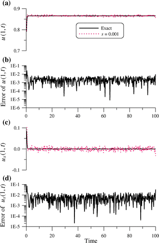
Under the following parameters m = 401, n = 41, and under a noise with s = 0.001, we solve the above inverse problem to recover initial condition and two right-end boundary conditions.

In Figure 8, we compare the recovered temperature and heat flux at x = 1 with exact solution, which are accurate with the maximum error and RMSE1 of initial condition being 8.56 × 10⁻³ and 5.89 × 10⁻³, respectively, the maximum error and RMSE2 of right-end temperatures are 2.52 × 10⁻² and 3.18 × 10⁻³, respectively, and the maximum error and RMSE3 of right-end heat flux are 7.05 × 10⁻² and 8.34 × 10⁻³, respectively. The accuracy as can be seen from Figure 8 is good in the order of O(10⁻¹)－O(10⁻⁶) even under the moderate noisy effect. Besides, the non-linear evolution equations are also useful in the mathematical modelling of non-linear phase-field transition system [74–82].

Figure 8. For example 7: (a) comparing numerical and exact right-end temperatures, (b) the numerical error of right-end temperatures, (c) comparing numerical and exact right-end heat fluxes, and (d) the numerical error of right-end heat fluxes.

3.8. Example 8

We further consider the 1-D NWS Equation [41]:(37) $$u_{xx}=u_t-u+u^4,\text{0}<x<\ell \text{,}0<t<T,$$(37)

and the exact solution u of Equations (2(2) $$u(0,t)=u_0(t)\text{,}$$(2) ), (3(3) $$u_x(0,t)=q_0(t),$$(3) ) and (37(37) $$u_{xx}=u_t-u+u^4,\text{0}<x<\ell \text{,}0<t<T,$$(37) ) is given by

(38) $$u(x,t)={\left\{0.5tanh\left[\frac{-3}{2\sqrt{10}}\left(x-\frac{7}{\sqrt{10}}t\right)\right]+0.5\right\}}^{2/3},\text{0}<x<1.2\text{,}0<t<100.$$(38)

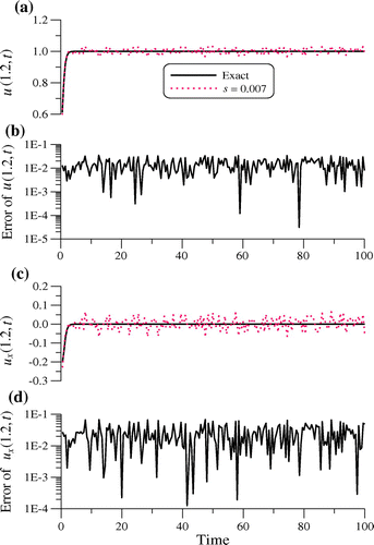
To give a stringent test of the two-stage GPS when utilized it on this numerical experiment, we add the non-linear source term in the order of four. Under the following parameters m = 201, n = 37 and under a noise with s = 0.007, we resolve the above inverse problem to retrieve initial condition and two right-end boundary conditions.

In Figure 9, we compare the recovered temperature and heat flux at x = 1.2 with exact solution, which are accurate with the maximum error and RMSE1 of initial condition being 1.25 × 10⁻² and 6.15 × 10⁻³, respectively, the maximum error and RMSE2 of right-end temperatures are 3.49 × 10⁻² and 1.69 × 10⁻², respectively, and the maximum error and RMSE3 of right-end heat flux are 6.79 × 10⁻² and 3.04 × 10⁻², respectively. The accuracy as shown in Figure 9 is good in the order of O(10⁻¹)－O(10⁻⁵) even under the moderate noisy effect. Moreover, to the authors’ best knowledge, there has been no report that numerical methods can calculate this equation very well as our algorithm.

Figure 9. For example 8: (a) comparing numerical and exact right-end temperatures, (b) the numerical error of right-end temperatures, (c) comparing numerical and exact right-end heat fluxes, and (d) the numerical error of right-end heat fluxes.

4. Conclusions

The Cauchy problems of non-linear evolution equations have been well calculated by the formulation with a semi-discretization of the time coordinate of evolution equation in conjunction with the group preserving numerical integration scheme along the spatial direction. By utilizing a two-stage GPS, we can recover the temperature and heat flux very well for the Cauchy problems of non-linear evolution equations without initial data. Eight numerical instances were worked out, which presented that the proposed numerical integration schemes were applicable to these issues. Compared with Liu and Chang [72], the proposed approach is more robust to recover the initial temperatures and right-end temperatures and heat fluxes when the two left-end boundary conditions are under a quite large noise and a very large time span. Besides, the proposed method does not need the stabilization parameter to raise the accuracy of numerical solutions. The two-stage GPS can be extended to solve the Cauchy problems of non-linear evolution equations without initial data defined in an arbitrary plane area. These issues will be coped with in the near future.

Funding

This work was financially supported by the Ministry of Science and Technology of Taiwan [grant numbers MOST 104-2221-E-492-029].

Disclosure statement

No potential conflict of interest was reported by the authors.

References

- Satsuma J, In: Ablowitz M, Fuchssteiner B, Kruskal M, editors. Topics in soliton theory and exactly solvable nonlinear equations. Singapore: World Scientific; 1987.
- Wang XY, Zhu ZS, Lu YK. Solitary wave solutions of the generalized Burgers–Huxley equation. J Phys A Math Gen. 1990;23:271–274.10.1088/0305-4470/23/3/011
- Wazwaz A-M. Analytic study on Burgers, Fisher, Huxley equations and combined forms of these equations. Appl Math Comput. 2008;195:754–761.
- Deng X. Travelling wave solutions for the generalized Burgers–Huxley equation. Appl Math Comput. 2008;204:733–737.
- Babolian E, Saeidian J. Analytic approximate solutions to Burgers, Fisher, Huxley equations and two combined forms of these equations. Commun Nonlinear Sci Numer Simul. 2009;14:1984–1992.10.1016/j.cnsns.2008.07.019
- Molabahrami A, Khani F. The homotopy analysis method to solve the Burgers–Huxley equation. Nonlinear Anal Real World Appl. 2009;10:589–600.10.1016/j.nonrwa.2007.10.014
- Deng XJ, Yan ZZ, Han L-B. Travelling wave solutions for the generalized Burgers–Huxley equation with nonlinear terms of any order. Chin Phys B. 2009;18:3169–3173.
- Gao H, Zhao R-X. New exact solutions to the generalized Burgers–Huxley equation. Appl Math Comput. 2010;217:1598–1603.
- Zhou Y, Liu Q, Zhang W. Bounded traveling waves of the generalized Burgers–Huxley equation. Nonlinear Anal Theory Methods Appl. 2011;74:1047–1060.10.1016/j.na.2010.09.012
- Krisnangkura M, Chinviriyasit S, Chinviriyasit W. Analytic study of the generalized Burger’s–Huxley equation by hyperbolic tangent method. Appl Math Comput. 2012;218:10843–10847.
- Chen H, Zhang H. New multiple soliton solutions to the general Burgers–Fisher equation and the Kuramoto–Sivashinsky equation. Chaos Solitons Fractals. 2004;19:71–76.10.1016/S0960-0779(03)00081-X
- Ismail HNA, Raslan K, Abd Rabboh AA. Adomian decomposition method for Burger’s–Huxley and Burger’s–Fisher equations. Appl Math Comput. 2004;159:291–301.
- Wazwaz A-M. The tanh method for generalized forms of nonlinear heat conduction and Burgers–Fisher equations. Appl Math Comput. 2005;169:321–338.
- Wazwaz A-M. Traveling wave solutions of generalized forms of Burgers, Burgers–KdV and Burgers–Huxley equations. Appl Math Comput. 2005;169:639–656.
- El-Wakil SA, Abdou MA. Modified extended tanh-function method for solving nonlinear partial differential equations. Chaos Solitons Fractals. 2007;31:1256–1264.10.1016/j.chaos.2005.10.072
- Abbasbandy S. Soliton solutions for the Fitzhugh–Nagumo equation with the homotopy analysis method. Appl Math Model. 2008;32:2706–2714.10.1016/j.apm.2007.09.019
- Abdusalam HA. Analytic and approximate solutions for Nagumo telegraph reaction diffusion equation. Appl Math Comput. 2004;157:515–522.
- Aronson DG, Weinberger HF. Multidimensional nonlinear diffusion arising in population genetics. Adv Math. 1978;30:33–76.10.1016/0001-8708(78)90130-5
- Browne P, Momoniat E, Mahomed FM. A generalized Fitzhugh–Nagumo equation. Nonlinear Anal. 2008;68:1006–1015.10.1016/j.na.2006.12.001
- Kawahara T, Tanaka M. Interactions of traveling fronts: an exact solution of a nonlinear diffusion equation. Phys Lett A. 1983;97:311–314.10.1016/0375-9601(83)90648-5
- Li H, Guo Y. New exact solutions to the Fitzhugh–Nagumo equation. Appl Math Comput. 2006;180:524–528.
- Aasaraai A. Analytic solution for Newell–Whitehead–Segel equation by differential transform method. Middle-East J Sci Res. 2011;10:270–273.
- Batiha B, Noorani MSM, Hashim I. Numerical simulation of the generalized Huxley equation by He’s variational iteration method. Appl Math Comput. 2007;186:1322–1325.
- Hashemi SH, Mohammadi Daniali HR, Ganji DD. Numerical simulation of the generalized Huxley equation by He’s homotopy perturbation method. Appl Math Comput. 2007;192:157–161.
- Darvishi MT, Kheybari S, Khani F. Spectral collocation method and Darvishi’s preconditionings to solve the generalized Burgers–Huxley equation. Commun Nonlinear Sci Numer Simul. 2008;13:2091–2103.10.1016/j.cnsns.2007.05.023
- Khattak AJ. A computational meshless method for the generalized Burger’s–Huxley equation. Appl Math Model. 2009;33:3718–3729.10.1016/j.apm.2008.12.010
- Macías-Díaz JE, Ruiz-Ramírez J, Villa J. The numerical solution of a generalized Burgers–Huxley equation through a conditionally bounded and symmetry-preserving method. Comput Math Appl. 2011;61:3330–3342.10.1016/j.camwa.2011.04.022
- Zhang R, Yu X, Zhao G. The local discontinuous Galerkin method for Burger’s–Huxley and Burger’s–Fisher equations. Appl Math Comput. 2012;218:8773–8778.
- Çelik İ. Haar wavelet method for solving generalized Burger’s–Huxley equation. Arab J Math Sci. 2012;18:25–37.
- Dehghan M, Saray BN, Lakestani M. Three methods based on the interpolation scaling functions and the mixed collocation finite difference schemes for the numerical solution of the nonlinear generalized Burgers–Huxley equation. Math Comput Model. 2012;55:1129–1142.
- Ervin VJ, Macías-Díaz JE, Ruiz-Ramírez J. A positive and bounded finite element approximation of the generalized Burgers–Huxley equation. J Math Anal Appl. 2015;424:1143–1160.10.1016/j.jmaa.2014.11.047
- Duan Y, Kong L, Zhang R. A lattice Boltzmann model for the generalized Burgers–Huxley equation. Phys A. 2012;391:625–632.10.1016/j.physa.2011.08.034
- Kaya D, El-Sayed SM. A numerical simulation and explicit solutions of the generalized Burgers–Fisher equation. Appl Math Comput. 2004;152:403–413.
- Zhu CG, Kang WS. Numerical solution of Burgers–Fisher equation by cubic B-spline quasi-interpolation. Appl Math Comput. 2010;216:2679–2686.
- Javidi M. A modified Chebyshev pseudospectral DD algorithm for the GBH equation. Comput Math Appl. 2011;62:3366–3377.10.1016/j.camwa.2011.08.051
- Soheili AR, Kerayechian A, Davoodi N. Adaptive numerical method for Burgers-type nonlinear equations. Appl Math Comput. 2012;219:3486–3495.
- Zhao T, Li C, Zang Z, et al. Chebyshev–Legendre pseudo-spectral method for the generalized Burgers–Fisher equation. Appl Math Model. 2012;36:1046–1056.10.1016/j.apm.2011.07.059
- Xiang X, Wang Z, Shi B. Modified lattice Boltzmann scheme for nonlinear convection diffusion equations. Commun Nonlinear Sci Numer Simul. 2012;17:2415–2425.10.1016/j.cnsns.2011.09.036
- Bhrawy AH. A Jacobi–Gauss–Lobatto collocation method for solving generalized Fitzhugh–Nagumo equation with time-dependent coefficients. Appl Math Comput. 2013;222:255–264.
- Jiwari R, Gupta RK, Kumar V. Polynomial differential quadrature method for numerical solutions of the generalized Fitzhugh–Nagumo equation with time-dependent coefficients. Ain Shams Eng J. 2014;5:1343–1350.10.1016/j.asej.2014.06.005
- Nourazar SS, Soori M, Nazari-Golshan A. On the exact solution of Newell–Whitehead–Segel equation using the homotopy perturbation method. Aust J Basic Appl Sci. 2011;5:1400–1411.
- Ezzati R, Shakibi K. Using Adomian’s decomposition and multi-quadric quasi-interpolation methods for solving Newell–Whitehead equation. Proc Comput Sci. 2011;3:1043–1048.10.1016/j.procs.2010.12.171
- Macías-Díaz JE, Ruiz-Ramírez J. A non-standard symmetry-preserving method to compute bounded solutions of a generalized Newell–Whitehead–Segel equation. Appl Numer Math. 2011;61:630–640.10.1016/j.apnum.2010.12.008
- Pue-on P. Laplace adomian decomposition method for solving Newell–Whitehead–Segel equation. Appl Math Sci. 2013;7:6593–6600.10.12988/ams.2013.310603
- Saravanan A, Magesh N. A comparison between the reduced differential transform method and the Adomian decomposition method for the Newell–Whitehead–Segel equation. J Egypt Math Soc. 2013;21:259–265.10.1016/j.joems.2013.03.004
- Jassim HK. Homotopy perturbation algorithm using Laplace transform for Newell–Whitehead–Segel equation. Int J Adv Appl Math Mech. 2015;2:8–12.
- Aminikhah H, Alavi J. Numerical study of the nonlinear Cauchy diffusion problem and Newell-Whitehead equation via cubic B-spline quasi-interpolation. Iran J Numer Anal Optim. 2015;5:63–72.
- Liu C-S. Cone of non-linear dynamical system and group preserving schemes. Int J Non-Linear Mech. 2001;36:1047–1068.10.1016/S0020-7462(00)00069-X
- Lee HC, Liu C-S. The fourth-order group preserving methods for the integrations of ordinary differential equations. Comput Model Eng Sci. 2009;41:1–5.10.1063/1.3160130
- Liu C-S. Nonstandard group-preserving schemes for very stiff ordinary differential equations. Comput Model Eng Sci. 2005;9:255–272.
- Liu C-S. Preserving constraints of differential equations by numerical methods based on integrating factors. Comput Model Eng Sci. 2006;12:83–107.
- Chen Y-W, Liu C-S, Chang J-R. A chaos detectable and time step-size adaptive numerical scheme for non-linear dynamical systems. J Sound Vibr. 2007;299:977–989.10.1016/j.jsv.2006.08.028
- Liu C-S. An efficient backward group preserving scheme for the backward in time Burgers equation. Comput Model Eng Sci. 2006;12:55–65.
- Liu C-S. A group preserving scheme for Burgers equation with very large Reynolds number. Comput Model Eng Sci. 2006;12:197–211.
- Liu C-S. The Lie-group shooting method for nonlinear two-point boundary value problems exhibiting multiple solutions. Comput Model Eng Sci. 2006;13:149–163.
- Liu C-S. Efficient shooting methods for the second order ordinary differential equations. Comput Model Eng Sci. 2006;15:69–86.
- Liu C-S. The Lie-group shooting method for singularly perturbed two-point boundary value problems. Comput Model Eng Sci. 2006;15:179–196.
- Liu C-S. The computations of large rotation through an index two nilpotent matrix. Comput Model Eng Sci. 2006;16:157–175.
- Liu C-S. New integrating methods for time-varying linear systems and Lie-group computations. Comput Model Eng Sci. 2007;20:157–175.
- Liu C-S, Chang C-W, Chang J-R. Past cone dynamics and backward group preserving schemes for backward heat conduction problems. Comput Model Eng Sci. 2006;12:67–81.
- Liu C-S, Chang J-R, Chang C-W. The Lie-group shooting method for steady-state Burgers equation with high Reynolds number. J Hydrodyn Ser B. 2006;18:367–372.10.1016/S1001-6058(06)60080-2
- Liu C-S, Chang C-W, Chang J-R. A new shooting method for solving boundary layer equations in fluid mechanics. Comput Model Eng Sci. 2008;32:1–15.
- Liu C-S, Chang C-W, Chang J-R. The backward group preserving scheme for 1D backward in time advection-dispersion equation. Numer Methods Partial Differ Equ. 2010;26:61–80.10.1002/num.v26:1
- Chang C-W, Liu C-S, Chang J-R. A group preserving scheme for inverse heat conduction problems. Comput Model Eng Sci. 2015;10:13–38.
- Chang C-W, Chang J-R, Liu C-S. The Lie-group shooting method for boundary layer equations in fluid mechanics. J Hydrodyn Ser B. 2006;18:103–108.10.1016/S1001-6058(06)60038-3
- Chang J-R, Liu C-S, Chang C-W. A new shooting method for quasi-boundary regularization of backward heat conduction problems. Int J Heat Mass Transfer. 2007;50:2325–2332.10.1016/j.ijheatmasstransfer.2006.10.050
- Chang C-W, Liu C-S, Chang J-R. The Lie-group shooting method for quasi-boundary regularization of backward heat conduction problems. ICCES Online J. 2007;3:69–80.
- Chang C-W, Chang J-R, Liu C-S. The Lie-group shooting method for solving classical Blasius flat-plate problem. Comput Mater Cont. 2008;7:139–153.
- Chang C-W, Liu C-S, Chang J-R. A new shooting method for quasi-boundary regularization of multi-dimensional backward heat conduction problems. J Chin Inst Eng. 2009;32:307–318.10.1080/02533839.2009.9671510
- Liu C-S, Chang C-W. A Lie-group adaptive method to identify the radiative coefficients in parabolic partial differential equations. Comput Mater Cont. 2011;25:107–134.
- Liu C-S, Chang C-W. A novel mixed group preserving scheme for the inverse Cauchy problem of elliptic equations in annular domains. Eng Anal Boundary Elem. 2012;36:211–219.10.1016/j.enganabound.2011.08.001
- Liu C-S, Chang C-W. A simple algorithm for solving Cauchy problem of nonlinear heat equation without initial value. Int J Heat Mass Transfer. 2015;80:562–569.10.1016/j.ijheatmasstransfer.2014.09.053
- Hariharan G, Kannan K, Sharma KR. Haar wavelet method for solving Fisher’s equation. Appl Math Comput. 2009;211:284–292.
- Arnăutu V, Morosanu C. Numerical approximation for the phase-field transition system. Int J Comput Math. 1996;62:209–221.10.1080/00207169608804538
- Morosanu C. Approximation of the phase-field transition system via fractional steps method. Numer Funct Anal Optim. 1997;18:623–648.10.1080/01630569708816782
- Morosanu C, Motreanu D. Uniqueness and approximation for the nonlinear parabolic equation in Caginalp’s model. Int J Appl Math. 2000;2:113–129.
- Benincasa T, Morosanu C. Fractional steps scheme to approximate the phase-field transition system with nonhomogeneous Cauchy–Neumann boundary conditions. Numer Funct Anal Optim. 2009;30:199–213.10.1080/01630560902841120
- Benincasa T, Morosanu C. A product formula approach to an inverse problem governed by nonlinear phase-field transition system. Case 1D. ROMAI J. 2010;6:15–26.
- Morosanu C. Cubic spline method and fractional steps schemes to approximate the phase-field system with non-homogeneous Cauchy–Neumann boundary conditions. ROMAI J. 2012;8:73–91.
- Morosanu C, Moşneagu A-M. On the numerical approximation of the phase-field system with non-homogeneous Cauchy–Neumann boundary conditions. Case 1D. ROMAI J. 2013;9:91–110.
- Morosanu C, Gheorghiu CI. Accurate spectral solutions to a phase-field transition system. ROMAI J. 2014;10:89–99.
- Miranville A, Morosanu C. Analysis of an iterative scheme of fractional steps type associated to the nonlinear phase-field equation with non-homogeneous dynamic boundary conditions. Dis Cont Dyn Syst – Ser S. 2016;9:537–556. 10.3939/dcdss.2016011